R E S E A R C H
Open Access
Modified hybrid decomposition of the
augmented Lagrangian method with larger
step size for three-block separable convex
programming
Min Sun
1,2*and Yiju Wang
2*Correspondence: [email protected] 1School of Mathematics and
Statistics, Zaozhuang University, Zaozhuang, P.R. China
2School of Management, Qufu
Normal University, Qufu, P.R. China
Abstract
The Jacobian decomposition and the Gauss–Seidel decomposition of augmented Lagrangian method (ALM) are two popular methods for separable convex programming. However, their convergence is not guaranteed for three-block separable convex programming. In this paper, we present a modified hybrid decomposition of ALM (MHD-ALM) for three-block separable convex programming, which first updates all variables by a hybrid decomposition of ALM, and then corrects the output by a correction step with constant step size
α
∈(0, 2 –√2) which is much less restricted than the step sizes in similar methods. Furthermore, we show that 2 –√2 is the optimal upper bound of the constant step sizeα. The rationality of
MHD-ALM is testified by theoretical analysis, including global convergence, ergodic convergence rate, nonergodic convergence rate, and refined ergodic convergence rate. MHD-ALM is applied to solve video background extraction problem, and numerical results indicate that it is numerically reliable and requires less computation.Keywords: The augmented Lagrangian method; Three-block separable convex programming; Step size; Global convergence
1 Introduction
Many problems encountered in applied mathematics area can be formulated as separable convex programming, such as basis pursuit (BP) problem [1–3], video background extrac-tion problem [4–7], image decomposiextrac-tion [8–10], and so on. Thus the solving of separa-ble convex programming plays a fundamental role in applied mathematics and has drawn persistent attention. In the existing literature, several forms of separable convex program-ming have been investigated [11–15], in which the following three-block separable convex programming rouses more interest:
min
3
i=1
θi(xi) 3
i=1
Aixi=b,xi∈Xi,i= 1, 2, 3
, (1)
whereθi:Rni→(–∞, +∞] (i= 1, 2, 3) are lower semicontinuous proper convex func-tions,Ai∈Rl×ni(i= 1, 2, 3) andb∈Rl,Xi(i= 1, 2, 3) are nonempty closed convex sets in
Rni(i= 1, 2, 3). Throughout this paper, we assume that the solution set of problem (1) is
nonempty.
The Lagrangian and augmented Lagrangian functions of problem (1) are defined, re-spectively, as
L(x1,x2,x3,λ) = 3
i=1
θi(xi) –
λ,
3
i=1
Aixi–b
, (2)
Lβ(x1,x2,x3,λ) =L(x1,x2,x3,λ) +
β 2
3
i=1
Aixi–b
2
, (3)
whereλ∈Rlis the Lagrange multiplier associated with the linear constraints in (1), and β> 0 is a penalty parameter. Applying the augmented Lagrangian method (ALM) [16] to problem (1), we can obtain the following iterative scheme:
⎧ ⎨ ⎩
(xk1+1,xk2+1,x3k+1) =argmin{Lβ(x1,x2,x3,λk)|x1∈X1,x2∈X2,x3∈X3},
λk+1=λk–β(A1xk1+1+A2xk2+1+A3xk3+1–b).
(4)
Obviously, three variablesx1,x2,x3 are all involved in the minimization problem of (4),
which makes the method often hard to implement. One technique to handle this is to split the subproblem into several small scale subproblems. Based on this, if we split it in a Gauss–Seidel manner and adopt the famous alternating direction method of multiplier (ADMM) [11], we obtain the following iterative scheme:
⎧ ⎪ ⎪ ⎪ ⎪ ⎪ ⎨ ⎪ ⎪ ⎪ ⎪ ⎪ ⎩
xk1+1=argmin{Lβ(x1,x2k,xk3,λk)|x1∈X1},
xk+1
2 =argmin{Lβ(xk1+1,x2,xk3,λk)|x2∈X2},
x3k+1=argmin{Lβ(xk1+1,x2k+1,x3,λk)|x3∈X3},
λk+1=λk–β(A1xk1+1+A2xk2+1+A3xk3+1–b).
(5)
On the other hand, if we split it in a Jacobian manner, we get the following full parallel iterative scheme:
⎧ ⎪ ⎪ ⎪ ⎪ ⎪ ⎨ ⎪ ⎪ ⎪ ⎪ ⎪ ⎩
xk1+1=argmin{Lβ(x1,x2k,xk3,λk)|x1∈X1},
xk+1
2 =argmin{Lβ(xk1,x2,xk3,λk)|x2∈X2},
xk3+1=argmin{Lβ(xk1,xk2,x3,λk)|x3∈X3},
λk+1=λk–β(A1xk1+1+A2xk2+1+A3xk3+1–b).
(6)
Compared with the regularization method, the prediction-correction method has at-tracted extensive interest, and during the past decades many scholars have performed studies in this direction. For example, Heet al.[24] proposed an ADMM-based contrac-tion type method for solving multi-block separable convex programming, which first gen-erates a temporal iterate by (5), and then corrects it with a Gaussian back substitution procedure. Later, Heet al.[12] developed a full Jacobian decomposition of the augmented Lagrangian method for solving multi-block separable convex programming, which first generates a temporal iterate by (6), and then corrects it with a constant step size or varying step size. Different from the above, Hanet al.[13] proposed a partial splitting augmented Lagrangian method for solving three-block separable convex programming, which first updates the primal variablesx1,x2,x3in a partially-parallel manner, and then correctsx3,
λwith a constant step size. Later, Wanget al.[25] presented a proximal partially-parallel splitting method for solving multi-block separable convex programming, which first up-dates all primal variables in a partially-parallel manner, and then corrects the output with a constant step size or varying step size. Quite recently, Changet al.[26] proposed a con-vergent prediction-correction-based ADMM in which more minimization problems are involved. In conclusion, the above iteration schemes first generate a temporal iterate by (5) or (6) or their variants, and then generate the new iterate by correcting the temporal iterate with varying step size or a constant step size.
Varying step size needs to be dynamically updated at each iteration, which might be computationally demanding for large-scale (1). Hence in this paper, we consider the prediction-correction method with constant step size for solving problem (1). To the best of our knowledge, Heet al.[12] first proposed a prediction-correction method with con-stant step size for solving (1), and they proved that the upper bound of the concon-stant step size is 0.2679. By taking a hybrid splitting of (4) as the prediction step, Wanget al.[25] relaxed the upper bound of the constant step size to 0.3670 and Hanet al.[13] further relaxed it to 0.3820. In practice, to enhance the numerical efficiency of the corresponding iteration method, larger values of the step size are preferred as long as the convergence is still guaranteed [26]. In this paper, based on the methods in [12,13,25], we propose a modified hybrid decomposition of the augmented Lagrangian method with constant step size, whose upper bound is relaxed to 0.5858.
The rest of this paper is organized as follows. Section2lists some notations and basic results. In Sect. 3, we present a modified hybrid decomposition of the augmented La-grangian method with larger step size for problem (1) and establish its global convergence and refined convergence rate. Furthermore, a simple example is given to illustrate that 2 –√2∼= 0.5858 is the optimal upper bound of the constant step size in MHD-ALM. In Sect.4, some numerical results are given to demonstrate the numerical advantage of larger step size. Finally, a brief conclusion including some possible future works is drawn in Sect.5.
2 Preliminaries
In this section, we give some notations and basic results about the minimization problem (1), which will be used in the forthcoming discussions.
Throughout this paper, we define the following notations:
θ(x) =θ1(x1) +θ2(x2) +θ3(x3)
and
A= (A1,A2,A3), X=X1×X2×X3, V=X2×X3×Rl, W=X×Rl.
Definition 2.1 A tuple (x∗,λ∗)∈Wis called a saddle point of the Lagrangian function (2) if it satisfies the inequalities
Lλ∈Rl
x∗,λ≤Lx∗,λ∗≤Lx∈Xx,λ∗. (7)
Solving problem (1) is equivalent to finding a saddle point ofL(x,λ) [26,27]. Therefore, to solve (1), we only need to solve the two inequalities in (7), which can be written as the following mixed variational inequality:
θ(x) –θx∗+w–w∗Fw∗≥0, ∀w∈W, (8)
where
F(w) =
⎛ ⎜ ⎜ ⎜ ⎝
–A1λ –A2λ –A3λ
3
i=1Aixi–b
⎞ ⎟ ⎟ ⎟ ⎠=
–Aλ Ax–b
=
0 –A
A 0
x
λ
–
0
b
. (9)
BecauseF(w) is a linear mapping with skew-symmetric coefficient matrix, it satisfies the following property:
w–wFw=w–wF(w), ∀w,w∈W. (10)
The mixed variational inequality (8) is denoted byMVI(W,F,θ), whose solution set is denoted byW∗, which is nonempty from the assumption on problem (1).
To solveMVI(W,F,θ), Heet al.[28] presented the following prototype algorithm:
A prototype algorithm for MVI(W, F,θ), denoted by ProAlo:
Prediction: For givenvk, findwˆk∈WandQsatisfying
θ(x) –θxˆk+w–wˆkFwˆk≥v–vˆkQvk–vˆk, ∀w∈W, (11)
where the matrixQhas the property: (Q+Q) is positive definite.
Correction: Determine a nonsingular matrixM, a scalarα> 0, and generate the new iteratevk+1via
vk+1=vk–αMvk–vˆk. (12)
Condition 2.1 The matricesQ,Min the ProAlo satisfy that the three matricesQ+Q,
Under Condition2.1, Heet al.[28] established the convergence results of ProAlo, includ-ing the global convergence, the worst-caseO(1/t) convergence rate in ergodic or noner-godic sense, wheretis the iteration counter. See Theorems 3.3, 4.2, 4.5 in [28].
To end this section, we give the following lemma which will be used in the subsequent section.
Lemma 2.1([27]) LetX⊆Rnbe a closed nonempty convex set,θ(x)and f(x)be two
con-vex functions.If the functionθ(x)is nondifferentiable,the function f(x)is differentiable,
and the solution set of the problemmin{θ(x) +f(x)|x∈X}is nonempty,then
x∗∈argminθ(x) +f(x)|x∈X
if and only if
x∗∈X, θ(x) –θx∗+x–x∗∇fx∗≥0, ∀x∈X.
3 Algorithm and its convergence
In this section, we give the process of the modified hybrid decomposition of the augmented Lagrangian method (MHD-ALM) for three-block separable convex programming (1) and establish its convergence results, including global convergence, ergodic convergence rate, nonergodic convergence rate, and refined ergodic convergence rate.
Algorithm: MHD-ALM
Step0. Let parametersα∈(0, 2 –√2),β> 0, tolerance errorε> 0. Choose an initial point v0= (x02,x03,λ0)∈V. Setk= 0.
Step1. Compute the prediction iteratew˜k= (x˜k
1,x˜k2,x˜k3,λ˜k)via
⎧ ⎪ ⎪ ⎪ ⎪ ⎪ ⎨ ⎪ ⎪ ⎪ ⎪ ⎪ ⎩
˜
xk
1=argmin{Lβ(x1,xk2,xk3,λk)|x1∈X1},
˜
xk2=argmin{Lβ(˜xk1,x2,xk3,λk)|x2∈X2},
˜
xk
3=argmin{Lβ(x˜k1,xk2,x3,λk)|x3∈X3},
˜
λk=λk–β(A
1x˜k1+A2x˜2k+A3x˜k3–b).
(13)
Step2. Ifmax{A2xk2–A2x˜k2,A3xk3–A3x˜k3,λk–λ˜k} ≤ε, then stop; otherwise, go to
Step 3.
Step3. Generate the new iteratewk+1= (xk+1
1 ,xk2+1,x3k+1,λk+1)by
⎧ ⎪ ⎪ ⎪ ⎪ ⎪ ⎨ ⎪ ⎪ ⎪ ⎪ ⎪ ⎩
xk+1 1 =x˜k1,
xk2+1=xk2–α(xk2–x˜k2),
xk+1
3 =xk3–α(xk3–x˜k3),
λk+1=λk–α(λk–λ˜k).
(14)
Replacek+ 1byk, and go to Step 1.
manner. Furthermore, the feasible set of the step sizeαin MHD-ALM is extended from (0, 0.2679) in [12], (0, 0.3820) in [13], (0, 0.3670) in [25] to (0, 0.5858).
The methods in [12,13,24–26] and MHD-ALM all fall into the algorithmic framework of prediction-correction methods. The main differences among these methods are: (i) in the prediction step, the methods in [24,26] update all the primal variables in a sequential order; the method in [12] updates all the primal variables in a parallel manner; the methods in [13,25] and MHD-ALM update all the primal variables in a partial parallel manner, i.e., they first updatex1and then updatex2,x3in a parallel manner; (ii) in the correction step,
the method in [13] updatesx3,λ; the method in [26] and MHD-ALM updatex2,x3,λ, and
the methods in [12,24,25] update all the variables.
The convergence analysis of MHD-ALM needs the following assumption and auxiliary sequence.
Assumption 3.1 The matricesA2,A3in problem (1) are both full column rank.
Define an auxiliary sequencewˆk= (ˆxk1,xˆk2,xˆk3,λˆk) as
ˆ
xki =x˜ki (i= 1, 2, 3), λˆk=λk–βA1x˜k1+A2xk2+A3xk3–b
. (15)
To prove the convergence results of MHD-ALM, we only need cast it into the ProAlo and ensure the following two conditions hold: (i) the generated sequence satisfying (11), (12); (ii) the resulting matricesQ,Msatisfying Condition2.1in Sect.2. We first verify the first condition. Based on Lemma2.1, we can derive the first order optimality conditions of the subproblems in (13), which are summarized in the following lemma.
Lemma 3.1 Let{wk}be the sequence generated by MHD-ALM and{ ˆwk}be defined as in
(15).Then it holds that
θ(x) –θxˆk+w–wˆkFwˆk≥v–vˆkQvk–vˆk, ∀w∈W, (16)
where the matrix Q is defined by
Q=
⎛ ⎜ ⎝
βA2A2 0 0
0 βA3A3 0
–A2 –A3 Il/β
⎞ ⎟
⎠. (17)
Proof Based on Lemma2.1and using the notation ofwˆkin (15), the first order optimality conditions for the three minimization problems in (13) can be summarized as the follow-ing inequalities:
θ1(x1) –θ1
ˆ
xk1+x1–xˆk1
–A1λˆk≥0, ∀x1∈X1,
θ2(x2) –θ2
ˆ
xk2+x2–xˆk2
–A2λˆk–βA2A2
xk2–xˆk2≥0, ∀x2∈X2,
θ3(x3) –θ3
ˆ
xk3+x3–xˆk3
–A3λˆk–βA3A3
Furthermore, the definition of the variableλˆkin (15) gives
λ–λˆk
A1xˆk1+A2xˆ2k+A3xˆk3–b+A2
xk2–xˆk2+A3
xk3–xˆk3+1 β
ˆ
λk–λk= 0, ∀λ∈Rl.
Adding the above four inequalities, rearranging terms, and using the definition of the ma-trixQ, the functionF(w), we can get the result (16). This completes the proof.
Remark3.2 Whenmax{A2xk2–A2x˜k2,A3xk3–A3x˜k3,λk–λ˜k}= 0, by (15), we getA2xk2= A2xˆk2,A3xk3=A3xˆ3k,λk=λˆk. Thus,Q(vk–vˆk) = 0. This and inequality (16) indicate that
θ(x) –θxˆk+w–wˆkFwˆk≥0, ∀w∈W.
Therefore,wk∈W∗, and the stopping criterion of MHD-ALM is reasonable.
By the definition ofλˆkin (15), the updating formula ofλ˜kcan be represented as
˜
λk=λk–βA1x˜k1+A2x˜k2+A3x˜k3–b
=λk–λk–λˆk–βA2
xk2–xˆk2+A3
xk3–xˆk3
=λk– (–βA2, –βA3,Il)
vk–ˆvk. This together with (14), (15) gives
⎧ ⎨ ⎩
xk+1 1 =x˜k1,
vk+1=vk–αM(vk–vˆk),
(18)
where the matrixMis defined as
M=
⎛ ⎜ ⎝
Il 0 0
0 Il 0
–βA2 –βA3 Il
⎞ ⎟
⎠. (19)
Now to establish the convergence results of MHD-ALM, we only need to verify that the matricesQ,Msatisfy Condition2.1in Sect.2.
Lemma 3.2 Let the matrices Q,M be defined as in(17)and(19).Ifα∈(0, 0.5858)and Assumption3.1hold,then we have
(i) the symmetric matrixQ+Qis positive definite;
(ii) the matrixH=QM–1is symmetric and positive definite;
(iii) the matrixG(α) =Q+Q–αMHMis symmetric and positive definite.
Proof (i) From the definition ofQ, we have
Q+Q=
⎛ ⎜ ⎝
2βA2A2 0 –A2
0 2βA3A3 –A3
–A2 –A3 2Il/β
Therefore, for anyv= (x2,x3,λ)= 0, we have
vQ+Qv= 2βA2x22+ 2βA3x32+ 2λ(A2x2+A3x3) +
2 βλ
2. (20)
• If(x2,x3) = 0, thenλ= 0, so by (20), we getv(Q+Q)v=β2λ
2> 0.
• If(x2,x3)= 0, then from (20) we get
vQ+Qv≥βA2x22+βA3x32> 0,
where the first inequality follows from the inequality2xy≥–(βx2+y2/β), and
the second inequality comes from Assumption3.1.
(ii) From the definition ofQ,M, we have
H=
⎛ ⎜ ⎝
βA2A2 0 0
0 βA3A3 0
0 0 Il/β
⎞ ⎟ ⎠,
which is obviously positive definite by Assumption3.1. (iii) Similarly, from the definition ofQ,M, we have
G(α) =
⎛ ⎜ ⎝
β(2 – 2α)A2A2 –αβA2A3 –(1 –α)A2
–αβA3A2 β(2 – 2α)A3A3 –(1 –α)A3
–(1 –α)A2 –(1 –α)A3 (2 –α)Il/β
⎞ ⎟ ⎠
=LR(α)L,
where
L=
⎛ ⎜ ⎝
√
βA2 0 0
0 √βA3 0
0 0 Il/
√ β
⎞ ⎟
⎠, R(α) =
⎛ ⎜ ⎝
(2 – 2α)Il –αIl –(1 –α)Il –αIl (2 – 2α)Il –(1 –α)Il –(1 –α)Il –(1 –α)Il (2 –α)Il
⎞ ⎟ ⎠.
This together with Assumption3.1implies that we only need to prove the matrixR(α) is positive definite. In fact, it can be written as
R(α) =
⎛ ⎜ ⎝
2 – 2α –α –(1 –α) –α 2 – 2α –(1 –α) –(1 –α) –(1 –α) 2 –α
⎞ ⎟ ⎠⊗Il,
where⊗denotes the matrix Kronecker product. Thus, we only need to prove the 3 order matrix
⎛ ⎜ ⎝
2 – 2α –α –(1 –α) –α 2 – 2α –(1 –α) –(1 –α) –(1 –α) 2 –α
is positive definite, whose three eigenvalues areλ1= 2 –α,λ2= 2 – 2α–
√
3α2– 4α+ 2,
λ3= 2 – 2α+
√
3α2– 4α+ 2. Then, solving the following three inequalities simultaneously
⎧ ⎪ ⎪ ⎨ ⎪ ⎪ ⎩
2 –α> 0,
2 – 2α–√3α2– 4α+ 2 > 0,
2 – 2α+√3α2– 4α+ 2 > 0,
we get 0 <α< 2 –√2∼= 0.5858. Therefore, the matrixGis positive definite for anyα∈
(0, 0.5858). This completes the proof.
Lemma3.2indicates that the matricesQ,Mdefined as in (17) and (19) satisfy Condi-tion2.1in Sect.2, and thus we get the following convergence results of MHD-ALM based on Theorems 3.3, 4.2, 4.5 in [28].
Theorem 3.1(Global convergence) Let{wk}be the sequence generated by MHD-ALM.
Then it converges to a vector w∞,which belongs toW∗.
Theorem 3.2(Ergodic convergence rate) Let{wk}be the sequence generated by
MHD-ALM,{ ˆwk}be the corresponding sequence defined in(15).Set
¯
wt=1
t
t
k=0
ˆ
wk.
Then,for any integer t≥1,we have
θx¯t–θ(x) +w¯t–wF(w)≤ 1 2αtv–v
02
H, ∀w∈W. (21)
Theorem 3.3(Nonergodic convergence rate) Let{wk}be the sequence generated by
MHD-ALM.Then,for any w∗∈W∗and integer t≥1,we have
Mvt–vˆt2H≤ 1 c0t
v0–v∗2H,
where c0> 0is a constant.
The term
1 2αtv–v
02 H
on the right-hand side of (21) is used to measure the ergodic convergence rate of MHD-ALM. However, it is not only independent of the distance between the initial iteratew0
Lemma 3.3 Let{wk}be the sequence generated by MHD-ALM.Then,for any w∈W,we
have
αθ(x) –θxˆk+w–wˆkFwˆk≥1
2v–v k+12
H–v–v k2
H
+α 2v
k–vˆk2 H. (22)
Proof The proof is similar to that of Lemma 3.1 in [28] and is omitted for brevity of this
paper. This completes the proof.
Theorem 3.4(Refined ergodic convergence rate) Let{wk}be the sequence generated by MHD-ALM,{ ˆwk}be the sequence defined in(15).Set
¯
wt=1
t
t–1
k=0
ˆ
wk.
Then,for any integer t≥1,there exists a constant c> 0such that
⎧ ⎨ ⎩
|θ(x¯t) –θ(x∗)| ≤ c 2αt, Ax¯t–b ≤ c
2αt.
Proof Choosew∗= (x∗,λ∗)∈W∗. Then, for anyλ∈Rl, we havew˜∗:= (x∗,λ)∈W. From the definition ofF(w) in (9), we have
˜
w∗–wˆkFwˆk
=w˜∗–wˆkFw˜∗
=
x∗–xˆk λ–λˆk
–Aλ Ax∗–b
= –λAx∗–Axˆk
=λAxˆk–b,
where the first equation follows from (10). Settingw=w˜∗in (22), we get
αθxˆk–θx∗–w˜∗–wˆkFwˆk≤1
2v˜
∗–vk2 H–v˜
∗–vk+12 H
–α 2v
k–vˆk2 H.
Combining the above two inequalities gives
αθxˆk–θx∗–λAxˆk–b≤1
2w˜
∗–wk2 H–v˜
∗–vk+12 H
–α 2v
k–vˆk2 H.
Summing the above inequality fromk= 0 tot– 1 yields
t–1
k=0
θxˆk–tθx∗–λ
A t–1
k=0
ˆ
xk–tb
≤ 1 2αv˜
Dividing both sides of the above inequality byt, we get
1
t
t–1
k=0
θxˆk–θx∗–λAx¯t–b≤ 1
2αtv˜ ∗–v02
H.
Then it follows from the convexity ofθi(i= 1, 2, 3) that
θx¯t–θx∗–λAx¯t–b≤ 1
2αt
y0–y∗
λ0–λ
2
H
, (23)
wherey0= (x0
2,x03),y∗= (x∗2,x∗3). Since (23) holds for anyλ, we can set
λ= – Ax¯ t–b
Ax¯t–b,
and consequently,
θx¯t–θx∗+Ax¯t–b ≤ 1 2αtsupλ≤1
y0–y∗
λ0–λ
2
H .
Set
c= sup
λ≤1
y0–y∗
λ0–λ
2
H ,
and we thus get
θx¯t–θx∗+Ax¯t–b≤ c
2αt.
Sincex∗∈X∗(hereX∗denotes the solution set of problem (1)), we have
θx¯t–θx∗≥0.
Combining the above two inequalities gives
⎧ ⎨ ⎩
|θ(¯xt) –θ(x∗)| ≤2cαt, Ax¯t–b ≤ c
2αt,
which completes the proof.
As mentioned in Sect.1, Heet al.[12] used a simple example to show that the iterative scheme (6) may diverge for two-block separable convex programming. If we setθ1= 0, A1= 0 in (1) and MHD-ALM, then MHD-ALM reduces to the method in [12]. In this
Example3.1 Consider the linear equation
x2+x3= 0. (24)
Obviously, the linear equation (24) is a special case of problem (1) with the specifications: θ1=θ2=θ3= 0,A1= 0,A2=A3= 1,b= 0,X1=X2=X3=R. Due toθ1= 0,A1= 0, in the
following we do not consider the variablex1. The solution set of the corresponding mixed
variation inequalities is
W∗=x∗ 2,x∗3,λ∗
|x∗2+x∗3= 0,λ∗= 0.
For MHD-ALM, we setβ= 1, the initial pointx0
2=x03= 0,λ0= 1, and choose
α∈ {0.20, 0.21, 0.22, . . . , 0.55}.
The stopping criterion is set as
maxxk2+xk3,λk≤10–5,
or the number of iterations exceeds 10,000.
[image:12.595.118.479.477.723.2]The numerical results are graphically shown in Fig.1, which illustrates that whenα≤ 0.5, the number of iterations is descending with respect toα, while whenα∈(0.5, 0.55), the number of iterations increases quickly. Therefore,α= 0.5 is optimal for this problem, and larger values ofα in its feasible set indeed can enhance the numerical performance of MHD-ALM. Of course, some extreme values, such as the values near the upper bound 0.5858, are not appropriate choices.
Now, we show that MHD-ALM may diverge forα≥2 –√2. By some simple manipula-tions, the iterative scheme of (13) and (14) for problem (24) can be written in the following compact form:
⎛ ⎜ ⎝
xk+1 2 xk+1
3
λk+1
⎞ ⎟ ⎠=P(α)
⎛ ⎜ ⎝ xk 2 xk 3 λk ⎞ ⎟
⎠, (25)
where
P(α) =
⎛ ⎜ ⎝
1 –α –α α –α 1 –α α
α α 1 – 2α
⎞ ⎟ ⎠.
Three eigenvalues of the matrixP(α) are
λ1= 1, λ2= 1 – 2α+
√
2α, λ3= 1 – 2α–
√ 2α.
Now let us consider the following two cases: (1) For anyα> 2 –√2, we have
λ3= 1 – (2 +
√
2)α< 1 – (2 +√2)(2 –√2) = –1.
Thenρ(P(α)) > 1 forα> 2 –√2, whereρ(P(α)) is the spectral radius ofP(α). Hence, the iterative scheme (25) withα> 2 –√2 is divergent for this problem.
(2) Forα= 2 –√2, by eigenvalue decomposition, the matrixP(2 –√2) can be decom-posed as
P(2 –√2) =VDV,
where
V=
⎛ ⎜ ⎝
–1/2 –√2/2 1/2 –1/2 √2/2 1/2 √
2/2 0 √2/2
⎞ ⎟
⎠, D=
⎛ ⎜ ⎝
–1 0 0 0 1 0 0 0 4√2 – 5
⎞ ⎟ ⎠.
Thus, by (25), we get
⎛ ⎜ ⎝
xk+1 2 xk+1
3
λk+1
⎞ ⎟ ⎠= ⎛ ⎜ ⎜ ⎝ – √
2((–1)k–(4√2–5)k) 4
–
√
2((–1)k–(4√2–5)k) 4 (–1)k
2 +
(4√2–5)k 2
⎞ ⎟ ⎟ ⎠,
from which it holds that
⎛ ⎜ ⎝
x22k x2k 3
λ2k
⎞ ⎟ ⎠→ ⎛ ⎜ ⎝ – √ 2 4 – √ 2 4 1 2 ⎞ ⎟ ⎠, ⎛ ⎜ ⎝
x22k+1 x2k+1
3
λ2k+1
⎞ ⎟ ⎠→ ⎛ ⎜ ⎝ √ 2 4 √ 2 4
–12
Hence, the iterative scheme (25) withα= 2 –√2 is also divergent for this problem. Overall, 2 –√2 is the optimal upper bound of the step sizeαin MHD-ALM.
Now let us consider some special cases and extensions of MHD-ALM:
(1) Problem (1) withθ1= 0,A1= 0 reduces to two-block separable convex programming,
which can be solved by MHD-ALM as follows:
⎧ ⎪ ⎪ ⎨ ⎪ ⎪ ⎩ ˜
xk2=argmin{Lβ(x2,xk3,λk)|x2∈X2},
˜
xk
3=argmin{Lβ(xk2,x3,λk)|x3∈X3},
˜
λk=λk–β(A
2x˜k2+A3x˜k3–b),
(26) and ⎧ ⎪ ⎪ ⎨ ⎪ ⎪ ⎩
xk+1
2 =xk2–α(xk2–x˜k2),
xk3+1=xk3–α(xk3–x˜k3),
λk+1=λk–α(λk–λ˜k).
(27)
Since the iterative scheme (26), (27) is a special case of MHD-ALM, it is convergent for anyα∈(0, 2 –√2). Furthermore, by Example3.1, 2 –√2 is the optimal upper bound of the constant step sizeαin (26), (27).
(2) Similarly, problem (1) withθ3= 0,A3= 0 also reduces to two-block separable convex
programming, which can be solved by MHD-ALM as follows:
⎧ ⎪ ⎪ ⎨ ⎪ ⎪ ⎩ ˜ xk
1=argmin{Lβ(x1,x2k,λk)|x1∈X1},
˜
xk2=argmin{Lβ(x˜k1,x2,λk)|x2∈X2},
˜
λk=λk–β(A
1x˜k1+A2x˜k2–b),
(28) and ⎧ ⎪ ⎪ ⎨ ⎪ ⎪ ⎩
xk1+1=x˜k1,
xk+1
2 =xk2–α(xk2–x˜k2),
λk+1=λk–α(λk–λ˜k).
(29)
Following a similar analysis procedure, we can prove that the iterative scheme (28), (29) is convergent for anyα∈(0, 1).
(3) Extending MHD-ALM to solve four-block separable convex programming:
min
4
i=1
θi(xi) 4
i=1
Aixi=b,xi∈Xi,i= 1, 2, 3, 4
,
we can get the following iterative scheme:
⎧ ⎪ ⎪ ⎪ ⎪ ⎪ ⎪ ⎪ ⎪ ⎨ ⎪ ⎪ ⎪ ⎪ ⎪ ⎪ ⎪ ⎪ ⎩ ˜
xk1=argmin{Lβ(x1,xk2,xk3,xk4,λk)|x1∈X1},
˜
xk
2=argmin{Lβ(x˜k1,x2,x3k,xk4,λk)|x2∈X2},
˜
xk3=argmin{Lβ(˜xk1,xk2,x3,xk4,λk)|x3∈X3},
˜
xk
4=argmin{Lβ(˜xk1,xk2,x3k,x4,λk)|x4∈X4},
˜
λk=λk–β(A1x˜k–b),
and
⎧ ⎪ ⎪ ⎪ ⎪ ⎪ ⎪ ⎪ ⎪ ⎨ ⎪ ⎪ ⎪ ⎪ ⎪ ⎪ ⎪ ⎪ ⎩
xk+1 1 =x˜k1,
xk2+1=xk2–α(xk2–x˜k2),
xk+1
3 =xk3–α(xk3–x˜k3),
xk4+1=xk4–α(xk4–x˜k4),
λk+1=λk–α(λk–λ˜k).
(31)
With similar reasoning, we can prove that the iterative scheme (30), (31) is convergent for anyα∈(0, 2 –√3).
4 Numerical results
In this section, we demonstrate the practical efficiency of MHD-ALM by applying it to recover low-rank and sparse components of matrices from incomplete and noisy obser-vation. Furthermore, to give more insight into the behavior of MHD-ALM, we compare it with the full Jacobian decomposition of the augmented Lagrangian method (FJD-ALM) [12] and the proximal partially parallel splitting method with constant step size (PPPSM) [25]. All experiments are performed on a Pentium(R) Dual-Core CPU [email protected] GHz PC with 4 GB of RAM running on 64-bit Windows operating system.
The mathematical model of recovering low-rank and sparse components of matrices from incomplete and noisy observation is [20]
min L,S,U
L∗+τS1+
1
2μP (U)
2
,
s.t.L+S+U=D,
(32)
whereD∈Rp×q is a given matrix,τ > 0 is a balancing parameter,μ> 0 is a penalty pa-rameter, ⊆ {1, 2, . . . ,p} × {1, 2, . . . ,q}is the index set of the observable entries ofD, and
P :Rp×q→Rp×qis the projection operator defined by
P (X)ij=
⎧ ⎨ ⎩
Xij, if (i,j)∈ ,
0, otherwise, 1≤i≤p, 1≤j≤q.
Problem (32) is a concrete model of the generic problem (1), and MHD-ALM is applicable. For this problem, the three minimization problems in (13) all admit closed-form solutions, which can be found in [20].
4.1 Simulation example
We generate the synthetic data of (32) in the same way as [5,20]. Specifically, letL∗,S∗
be the low-rank matrix, the sparse matrix, respectively, andrr,spr, andsrrepresent the ratios of the low-rank ratio ofL∗(i.e.,r/p), the number of nonzero entries ofS∗(i.e., S∗0/(pq)), and the observed entries (i.e.,| /(pq)), respectively. The observed part of the
matrixDis generated by the following Matlab scripts, in whichbis the vectorization ofD:
X=randn(m,rr∗m)∗randn(rr∗m,n); Omega=randperm(m∗n);
Y=zeros(m,n); L=roundmin(spr,sr)∗m∗n; nzp=Omega(1:L);
Y(nzp) =rand(L,1)∗2–1∗500;b=X+Y;
b=b(Omega); sigma=0.001; b=b+sigma∗randn(p,1);
In this experiment, we setτ= 1/√p,μ= p+√8pσ/10,β=P0.06(D|)1| , the initial iterate (L0,S0,U0,λ0) = (0, 0, 0, 0), and use the stopping criterion
max
˜
Lk–Lk 1 +Lk,
˜Sk–Sk 1 +Sk
< 10–4, (33)
or the number of iterations exceeds 500.
The parameters in the three tested methods are listed as follows:
FJD-ALM:α= 0.38.
PPPSM:Si= 0,H=βI,Q=I,α= 0.36.
MHD-ALM:α= 0.5.
In Tables1and2, we report the numerical results of three tested methods, in which the number of iterations (denoted by ‘Iter.’), the elapsed CPU time in seconds (denoted by ‘Time’), the relative error of the recovered low-rank matrix, and the relative error of the recovered sparse matrix are reported when the stopping criterion (33) is satisfied.
Numerical results in Tables1and2indicate that: (i) all methods successfully solved all the tested cases; (ii) both MHD-ALM and PPPSM perform better than FJD-ALM, and MHD-ALM performed the best. The reason maybe that FJD-ALM updates all the pri-mal variables in a parallel manner, while PPPSM and MHD-ALM update x2,x3 based
on the newest updated x1 to accelerate the convergence speed. Furthermore, the step
[image:16.595.118.478.536.731.2]sizeα of MHD-ALM is larger than that of PPPSM, and the latter is larger than that of FJD-ALM. Therefore, larger values ofαcan enhance the efficiency of the corresponding method.
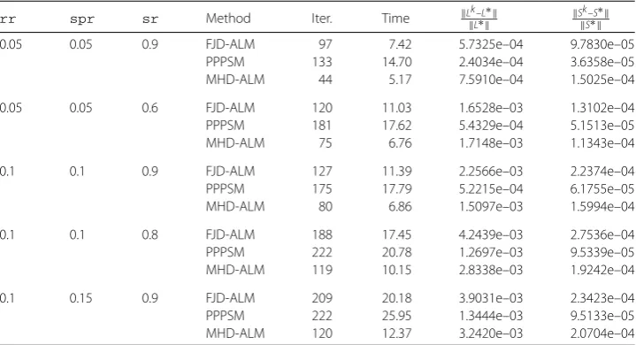
Table 1 Numerical comparisons between different algorithms forp=q= 500
rr spr sr Method Iter. Time Lk–LL∗∗ Sk–SS∗∗
0.05 0.05 0.9 FJD-ALM 97 7.42 5.7325e–04 9.7830e–05
PPPSM 133 14.70 2.4034e–04 3.6358e–05
MHD-ALM 44 5.17 7.5910e–04 1.5025e–04
0.05 0.05 0.6 FJD-ALM 120 11.03 1.6528e–03 1.3102e–04
PPPSM 181 17.62 5.4329e–04 5.1513e–05
MHD-ALM 75 6.76 1.7148e–03 1.1343e–04
0.1 0.1 0.9 FJD-ALM 127 11.39 2.2566e–03 2.2374e–04
PPPSM 175 17.79 5.2215e–04 6.1755e–05
MHD-ALM 80 6.86 1.5097e–03 1.5994e–04
0.1 0.1 0.8 FJD-ALM 188 17.45 4.2439e–03 2.7536e–04
PPPSM 222 20.78 1.2697e–03 9.5339e–05
MHD-ALM 119 10.15 2.8338e–03 1.9242e–04
0.1 0.15 0.9 FJD-ALM 209 20.18 3.9031e–03 2.3423e–04
PPPSM 222 25.95 1.3444e–03 9.5133e–05
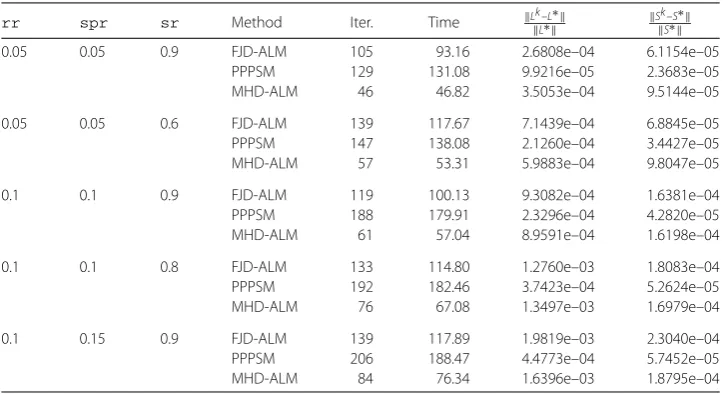
Table 2 Numerical comparisons between different algorithms forp=q= 1000
rr spr sr Method Iter. Time Lk–LL∗∗ Sk–SS∗∗
0.05 0.05 0.9 FJD-ALM 105 93.16 2.6808e–04 6.1154e–05
PPPSM 129 131.08 9.9216e–05 2.3683e–05
MHD-ALM 46 46.82 3.5053e–04 9.5144e–05
0.05 0.05 0.6 FJD-ALM 139 117.67 7.1439e–04 6.8845e–05
PPPSM 147 138.08 2.1260e–04 3.4427e–05
MHD-ALM 57 53.31 5.9883e–04 9.8047e–05
0.1 0.1 0.9 FJD-ALM 119 100.13 9.3082e–04 1.6381e–04
PPPSM 188 179.91 2.3296e–04 4.2820e–05
MHD-ALM 61 57.04 8.9591e–04 1.6198e–04
0.1 0.1 0.8 FJD-ALM 133 114.80 1.2760e–03 1.8083e–04
PPPSM 192 182.46 3.7423e–04 5.2624e–05
MHD-ALM 76 67.08 1.3497e–03 1.6979e–04
0.1 0.15 0.9 FJD-ALM 139 117.89 1.9819e–03 2.3040e–04
PPPSM 206 188.47 4.4773e–04 5.7452e–05
MHD-ALM 84 76.34 1.6396e–03 1.8795e–04
4.2 Application example
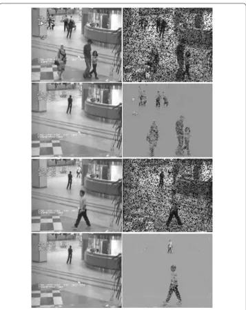
In this subsection, we apply the proposed method to solve the video background extrac-tion problem with missing and noisy data [29]. There is a video taken in an airport, which consists of 200 grayscale frames with each frame having 144×176 pixels. We need to sep-arate its background and foreground. Vectorizing all frames of the video, we get a matrix
D∈R25,344×50, and each column represents a frame. LetL,S∈R25,344×200 be the matrix
representations of its background and foreground (i.e., the moving objects), respectively. Then the rank ofLis equal to one exactly, andSshould be sparse with only a small num-ber of nonzero elements. We consider only a fraction entries ofDcan be observed, whose indices are collected in the index set . Then the background extraction problem with missing and noisy data can be casted as problem (32). In the experiment, the parameters in MHD-ALM are set asα= 0.5,β=0.005P (D|)1|, the parameters in (32) are set asτ = 1/√p, μ= 0.01, and the initial iterate (L0,S0,U0,λ0) = (0, 0, 0, 0). We use the same stopping
cri-terion as (33) with the tolerance 10–2.
Figure2displays the separation results of the 10th and 125th frames of the video with
sr= 0.7, which indicate that the proposed MHD-ALM successfully separates the back-ground and foreback-ground of the two frames.
5 Conclusion
In this paper, a hybrid decomposition of the augmented Lagrangian method is proposed for three-block separable convex programming, whose most important characteristic is that its correction step adopts a constant step size. We showed that the optimal upper bound of the constant step size is 2 –√2. Preliminary numerical results indicate that the proposed method is more efficient than similar methods in the literature.
The following two issues deserve further researching: (i) Due to Condition2.1being only a sufficient condition to ensure the convergence of the ProAlo, is 1 the optimal upper bound ofαin the iterative scheme (28), (29)? Similarly, is 2 –√2 the optimal upper bound ofαin the iterative scheme (30), (31)? (ii) If we choose different step sizes forx2,x3,λin the
Figure 2The 10th and 125th frames of the clean video and the corresponding corrupted frames with
sr= 0.7 (the top and third lines); the extracted background and foreground by MHD-ALM (the second and fourth lines)
Acknowledgements
The authors gratefully acknowledge the valuable comments of the editor and the anonymous reviewers.
Funding
This work is supported by the National Natural Science Foundation of China and Shandong Province (No. 11671228, 11601475, ZR2016AL05).
Availability of data and materials
The datasets used and/or analysed during the current study are available from the corresponding author on reasonable request.
Competing interests
Authors’ contributions
The first author provided the problems and gave the proof of the main results, and the second author finished the numerical experiment. All authors read and approved the final manuscript.
Publisher’s Note
Springer Nature remains neutral with regard to jurisdictional claims in published maps and institutional affiliations.
Received: 30 July 2018 Accepted: 21 September 2018
References
1. Chen, S.S., Donoho, D.L., Saunders, M.A.: Atomic decomposition by basis pursuit. SIAM J. Sci. Comput.20, 33–61 (1998)
2. Sun, M., Liu, J.: A proximal Peaceman–Rachford splitting method for compressive sensing. J. Appl. Math. Comput.50, 349–363 (2016)
3. Sun, M., Liu, J.: An accelerated proximal augmented Lagrangian method and its application in compressive sensing. J. Inequal. Appl.2017, 263 (2017)
4. Candés, E.J., Li, X.D., Ma, Y., Wright, J.: Robust principal component analysis? J. ACM58(1), 1–37 (2011) 5. Tao, M., Yuan, X.M.: Recovering low-rank and sparse components of matrices from incomplete and noisy
observations. SIAM J. Optim.21, 57–81 (2011)
6. Sun, M., Wang, Y.J., Liu, J.: Generalized Peaceman–Rachford splitting method for multiple-block separable convex programming with applications to robust PCA. Calcolo54(1), 77–94 (2017)
7. Sun, M., Sun, H.C., Wang, Y.J.: Two proximal splitting methods for multi-block separable programming with applications to stable principal component pursuit. J. Appl. Math. Comput.56, 411–438 (2018)
8. He, B.S., Yuan, X.M., Zhang, W.X.: A customized proximal point algorithm for convex minimization with linear constraints. Comput. Optim. Appl.56, 559–572 (2013)
9. He, B.S., Liu, H., Wang, Z.R., Yuan, X.M.: A strictly contractive Peaceman–Rachford splitting method for convex programming. SIAM J. Optim.24(3), 1011–1040 (2014)
10. He, B.S., Tao, M., Yuan, X.M.: A splitting method for separable convex programming. IMA J. Numer. Anal.35(1), 394–426 (2015)
11. Gabay, D., Mercier, B.: A dual algorithm for the solution of nonlinear variational problems via finite-element approximations. Comput. Math. Appl.2, 17–40 (1976)
12. He, B.S., Hou, L.S., Yuan, X.M.: On full Jacobian decomposition of the augmented Lagrangian method for separable convex programming. SIAM J. Optim.25(4), 2274–2312 (2015)
13. Han, D.R., Kong, W.W., Zhang, W.X.: A partial splitting augmented Lagrangian method for low patch-rank image decomposition. J. Math. Imaging Vis.51(1), 145–160 (2015)
14. Wang, Y.J., Zhou, G.L., Caccetta, L., Liu, W.Q.: An alternative Lagrange-dual based algorithm for sparse signal reconstruction. IEEE Trans. Signal Process.59, 1895–1901 (2011)
15. Wang, Y.J., Liu, W.Q., Caccetta, L., Zhou, G.L.: Parameter selection for nonnegative1matrix/tensor sparse
decomposition. Oper. Res. Lett.43, 423–426 (2015)
16. Hestenes, M.: Multiplier and gradient methods. J. Optim. Theory Appl.4, 303–320 (1969)
17. Chen, C.H., He, B.S., Ye, Y.Y., Yuan, X.M.: The direct extension of ADMM for multi-block convex minimization problems is not necessarily convergent. Math. Program.155(1), 57–79 (2016)
18. Sun, D.F., Toh, K.C., Yang, L.: A convergent 3-block semi-proximal alternating direction method of multipliers for conic programming with 4-type of constraints. SIAM J. Optim.25, 882–915 (2015)
19. He, B.S., Xu, H.K., Yuan, X.M.: On the proximal Jacobian decomposition of ALM for multiple-block separable convex minimization problems and its relationship to ADMM. J. Sci. Comput.66(3), 1204–1217 (2016)
20. Hou, L.S., He, H.J., Yang, J.F.: A partially parallel splitting method for multiple-block separable convex programming with applications to robust PCA. Comput. Optim. Appl.63(1), 273–303 (2016)
21. Wang, J.J., Song, W.: An algorithm twisted from generalized ADMM for multi-block separable convex minimization models. J. Comput. Appl. Math.309, 342–358 (2017)
22. Sun, M., Liu, J.: The convergence rate of the proximal alternating direction method of multipliers with indefinite proximal regularization. J. Inequal. Appl.2017, 19 (2017)
23. Sun, M., Sun, H.C.: Improved proximal ADMM with partially parallel splitting for multi-block separable convex programming. J. Appl. Math. Comput.58, 151–181 (2018)
24. He, B.S., Tao, M., Yuan, X.M.: Alternating direction method with Gaussian back substitution for separable convex programming. SIAM J. Optim.22, 313–340 (2012)
25. Wang, K., Desai, J., He, H.J.: A proximal partially-parallel splitting method for separable convex programs. Optim. Methods Softw.32(1), 39–68 (2017)
26. Chang, X.K., Liu, S.Y., Zhao, P.J., Li, X.: Convergent prediction-correction-based ADMM for multi-block separable convex programming. J. Comput. Appl. Math.335, 270–288 (2018)
27. He, B.S., Ma, F., Yuan, X.M.: Linearized alternating direction method of multipliers via positive-indefinite proximal regularization for convex programming. Optimization-online, 5569 (2016)
28. He, B.S., Yuan, X.M.: On the direct extension of ADMM for multi-block separable convex programming and beyond: from variational inequality perspective. Optimization-online, 4293 (2014)