Bernoulli numbers, convolution sums and congruences of coefficients for certain generating functions

R E S E A R C H

Open Access

Bernoulli numbers, convolution sums and

congruences of coefficients for certain

generating functions

Daeyeoul Kim

_{, Aeran Kim}

_{and Ayyadurai Sankaranarayanan}

*_{Correspondence:}

[email protected]

1_{National Institute for Mathematical}

Sciences, Yuseong-daero 1689-gil, Yuseong-gu, Daejeon, 305-811, South Korea

Full list of author information is available at the end of the article

Abstract

In this paper, we study the convolution sums involving restricted divisor functions, their generalizations, their relations to Bernoulli numbers, and some interesting applications.

MSC: 11B68; 11A25; 11A67; 11Y70; 33E99

Keywords: Bernoulli numbers; generating functions; divisor functions; convolution sums

1 Introduction

The Bernoulli polynomialsBk(x), which are usually defined by the exponential generating function

text

et_{– }=

∞

k= Bk(x)

tk

k!,

play an important role in different areas of mathematics, including number theory and the theory of finite differences. The Bernoulli polynomials satisfy the following well-known identities :

Bk(x+ ) –Bk(x) =kxk–, k≥,

d

dxBk(x) =kBk–(x), k≥,

and

N

j=

jk=Bk+(N+ ) –Bk+()

k+  , k≥.

We setBk=Bk(). It is obvious from the way the polynomialsBk(x) are constructed that all theBkare rational numbers. It can be shown thatBk+=  fork≥, and is alternatively

positive and negative for evenk. TheBkare called Bernoulli numbers.

Throughout the paper, we use the following arithmetical functions andq-series (some-times defined by product expressions). For any integerN≥,l,s∈N∪ {}, we define

σl(N) :=

d|N

dl, σ_s∗(N;p) := d|N

N

d≡ (modp)

ds, σ_s∗(N) :=σ_s∗(N; ) = d|N N/dodd

ds,

σs(N) :=

d|N

(–)d–ds, Si(N) := N–

k= ki.

Forq∈Cwith|q|< , we consider theq-series:

A(q) :=

∞

N=

σ_∗(N)qN, B(q) :=

∞

N=

σ_∗(N)qN, C(q) :=

∞

N=

σ_∗(N)qN,

∞

N=

a(N)qN:=q ∞

N=

 –qN –qN –qN –qN,

∞

N=

b(N)qN:=q ∞

N=

 –qN –qN,

∞

N=

c(N)qN:=q ∞

N=

 –qN –qN,

∞

N=

τ(N)qN:=q ∞

N=

 –qN,

∞

N=

l(N)qN:=q ∞

N=

 –qN –qN –qN.

The exact evaluation of the basic convolution sum

N–

k=

σ(k)σ(N–k)

first appeared in a letter from Besge to Liouville in . The evaluation of such sums also appear in the works of Glaisher, Lahiri, Lehmer, Ramanujan, and Skoruppa. For instance, Ramanujan [] obtained

N–

k=

σ(k)σ(N–k) =

 

σ(N) + ( – N)σ(N)

and

N–

k=

σ(k)σ(N–k) =

 

σ(N) + ( – N)σ(N) –σ(N)

()

using only elementary arguments. Fora,b,N∈N, Ramanujan showed that the sum

Sa,b(N) := N–

m=

σa(m)σb(N–m)

can be evaluated in terms of the quantities

for the nine pairs (a,b)∈N_satisfying

a+b= , , , , , a≤b,a≡b≡ (mod).

For explicit evaluations ofSa,b(N) for different pairs (a,b)∈Nsatisfying the above con-ditions stated, we refer to the papers of Ramanujan [], [], Huardet al.[], Lahiri [], and Glaisher [], respectively. Levit [] showed that the nine arithmetic evaluations ofSa,b(N) (witha,bboth odd) are the only ones using the theory of modular forms. In [], Lahiri has given  sums of the form

(m,...,mr)

m+···+nr=N

ma

 · · ·marrσb(m)· · ·σbr(mr),

where a, . . . ,ar∈N:=N∪ {}, b, . . . ,br∈N, each of which can be expressed as a fi-nite linear combination ofσ(N),σ(N), . . . ,σb+b+···+br+r–(N) with coefficients which are

polynomials inNof degree at mosta+· · ·+ar+r–  with rational coefficients. In , Huardet al.[] extended Melfi’s [] result to

k<N/

σ(k)σ(N– k)

= 

σ(N) +  σ

N



+( – N)  σ(N) –

 σ

N



,

k<N/

σ(k)σ(N– k)

= 

σ(N) +  σ

N



+( – N)  σ

N



–  σ(N),

()

whereNis an arbitrary positive integer.

Glaisher [, , ] extended Besge’s formula by replacingσ(N) in the convolution sum in

() by other arithmetical functions; for example, he obtained

 N–

k=

σ_∗(k)σ_∗(N–k) = σ(N) – σ N



– Nσ(N) + Nσ N



= σ_∗(N) –Nσ_∗(N) ()

and

N–

k=

σ_∗(k)σ_∗(N–k) =  

σ_∗(N) –Nσ_∗(N). ()

Recently, Hahn [] showed that



k<N

σ(k)σ(N–k) = –σ(N) + (N– )σ(N) +σ(N).

appear in the explicit evaluation of certain convolution sums. For instance, Lahiri (see []) proved that

N–

k=

k(N–k)σ(k)σ(N–k) =

 

Nσ(N) –τ(N)

and from Alaca and Williams (see []), we observe that

(k,m)∈N k+m=N

σ(k)σ(m)

= 

σ(N) +  σ

N



+  σ

N



+  σ

N



+  –

N



σ N



+  –

N



σ N



– 

a(N). ()

In [], Simsek (and also in [, (.)] Simsek along with Ozden and Cagul) has studied other aspects of the arithmetical functionσ(n) in connection with the classical Jacobi and

Euler functions. We also refer to Kim and Lee [, Lemma .] and [].

Thus the study of convolution sums and their applications is classical and they play an important role in number theory. The aim of this article is to first extend and generalize Glaishers formulas (stated in () and ()). We indeed study the sums (in Section )

N–

k=

σ_∗mkσ_∗n(N–k),

N–

k=

σ_∗mkσ_∗n(N–k),

N–

k=

σ_∗mkσ_∗n(N–k) and r+s+t=N

σ_∗mrσ_∗nsσ_∗lt.

Then, we study and evaluate (in Section ) sums of the type

N–

k=

σ_∗mk; σ_∗n(N–k);  and N–

k=

σ_∗mk; σ_∗n(N–k); .

As applications to our study and evaluations of convolution sums, we show thatA(q),B(q), andC(q) are connected by a second-order differential equation (see Theorem .).

In Section , we also prove some interesting congruence relations involving the coeffi-cients of modular-like functions and divisor functions (see Theorem .). As a sample, we obtain that ifN≡ (mod), then the congruence

τ(N)≡σ(N) (mod,,)

holds.

In Section , we present a generalization of Besge’s formula by considering certain com-binatorial convolution sums (see Theorem .). It should be noted that Proposition ., Theorem ., and Remark . exhibit amply the connection between the convolution sums and the Bernoulli numbers. Finally, we record special values ofa(N),τ(N),b(N),c(N), and

2 Some weighted convolution sums

Letf(a)g(b) :=_{f(a)g(b) +f(b)g(a)}. It is easily checked that

N–

k=

f(k)g(N–k) = N–

k=

f(k)g(N–k).

Lemma . For f,g:N→Cand N∈N,we have

N–

k=

kf(k)g(N–k) =N 

N–

k=

f(k)g(N–k).

Proof We observe that

N–

k=

kf(k)g(N–k) =  

N–

k=

kf(k)g(N–k) +f(N–k)g(k)

= 

N–

k=

(N–k)f(N–k)g(k) +f(k)g(N–k)

= N–

k=

(N–k)f(k)g(N–k).

Hence

 N–

k=

kf(k)g(N–k) =N

N–

k=

f(k)g(N–k)

and thus

N–

k=

kf(k)g(N–k) =N 

N–

k=

f(k)g(N–k).

Lemma . For f,g:N→Cand N∈N,we have

N–

k=

kf(k)g(N–k) = – N



N–

k=

f(N–k)g(k) +N 

N–

k=

kf(N–k)g(k).

Proof We note that

N–

k=

kf(k)g(N–k) = N–

k=

(N–k)f(N–k)g(k)

=N

N–

k=

f(N–k)g(k) – N

N–

k=

kf(N–k)g(k)

+ N

N–

k=

kf(N–k)g(k) – N–

k=

Then, for the second term on the right-hand side of (), we replace k by N–k in Lemma . and obtain

N–

k=

(N–k)f(N–k)g(k) =N 

N–

k=

f(N–k)g(k).

This shows that

N–

k=

kf(N–k)g(k) =N 

N–

k=

f(N–k)g(k).

So, () can be written as

N–

k=

kf(k)g(N–k) +f(N–k)g(k)

= –N



 N–

k=

f(N–k)g(k) + N

N–

k=

kf(N–k)g(k). ()

Here the left-hand side of () is

N–

k=

kf(k)g(N–k) +f(N–k)g(k)

= N–

k= k

 

f(k)g(N–k) +f(N–k)g(k)+ 

f(N–k)g(k) +f(k)g(N–k)

= N–

k=

kf(k)g(N–k) +f(N–k)g(k)=  N–

k=

kf(k)g(N–k).

Therefore we have

 N–

k=

kf(k)g(N–k) = – N



N–

k=

f(N–k)g(k) + N

N–

k=

kf(N–k)g(k).

This completes the proof.

Remark . In general, we can express

N–

k=

kl+f(k)g(N–k) fork∈N∪ {}

as a combination in terms of the sum

N–

k=

kjf(k)g(N–k) withj= , , , . . . ,k

Lemma . For l,N∈Nand f,g:N→C,we have

 + (–)l+ N–

k=

klf(k)g(N–k) = N–

k=

f(N–k)g(k) _l–

j= l j

(–)jkjNl–j

.

Proof We note that (forl∈N),

N–

k=

klf(k)g(N–k) = N–

k=

(N–k)lf(N–k)g(k)

= N–

k=

f(N–k)g(k) _l

j= l j

(–)jkjNl–j

= (–)l N–

k=

klf(N–k)g(k) + N–

k=

f(N–k)g(k) _l–

j= l j

(–)jkjNl–j

.

Observing the fact that

N–

k=

klf(k)g(N–k) = N–

k=

klf(N–k)g(k)

for anyl∈N, we obtain

 + (–)l+ N–

k=

klf(k)g(N–k) = N–

k=

f(N–k)g(k) _l–

j= l j

(–)jkjNl–j

.

This proves Lemma ..

Remark . By iteration process, in principle, the convolution sumN_k=–kl_f(k)g(N–k) can be evaluated for any oddl∈N.

Let

f(a)g(b)h(c) :=  

f(a)g(b)h(c) +f(a)g(c)h(b) +f(b)g(a)h(c)

+f(b)g(c)h(a) +f(c)g(a)h(b) +f(c)g(b)h(a).

Lemma . For f :N→Cand N∈N.Then we have

(r,s,t)∈N

r+s+t=N

rf(r)f(s)f(t) =N 

(r,s,t)∈N

r+s+t=N

f(r)f(s)f(t).

Proof From the cyclic transformation,r→s→t→r, we observe that

(r,s,t)∈N

r+s+t=N

rf(r)f(s)f(t) =

(r,s,t)∈N

r+s+t=N

sf(r)f(s)f(t) =

(r,s,t)∈N

r+s+t=N

Therefore, we have

(r,s,t)∈N

r+s+t=N

Nf(r)f(s)f(t) =

(r,s,t)∈N

r+s+t=N

(r+s+t)f(r)f(s)f(t) = 

(r,s,t)∈N

r+s+t=N

rf(r)f(s)f(t).

Now Lemma . follows.

Lemma . For f :N→Cand N∈N.Then we have(with g(m) =mf(m)for all m∈N)



(r,s,t)∈N

r+s+t=N

rf(r)f(s)f(t) =N (r,s,t)∈N

r+s+t=N

f(r)f(s)f(t) +  N–

t=

(r,s)∈N

r+s=N–t

g(r)g(s).

Proof As in Lemma ., again by the cyclic transformationr→s→t→r, we observe that

(r,s,t)∈N

r+s+t=N

rf(r)f(s)f(t) =

(r,s,t)∈N

r+s+t=N

sf(r)f(s)f(t) =

(r,s,t)∈N

r+s+t=N

tf(r)f(s)f(t) ()

and

(r,s,t)∈N

r+s+t=N

rsf(r)f(s)f(t) =

(r,s,t)∈N

r+s+t=N

stf(r)f(s)f(t) =

(r,s,t)∈N

r+s+t=N

trf(r)f(s)f(t). ()

Therefore, we get (from () and ())

(r,s,t)∈N

r+s+t=N

nf(r)f(s)f(t) = 

(r,s,t)∈N

r+s+t=N

rf(r)f(s)f(t) + 

(r,s,t)∈N

r+s+t=N

rsf(r)f(s)f(t)

= 

(r,s,t)∈N

r+s+t=N

rf(r)f(s)f(t) +  N–

t=

f(t)

(r,s)∈N

r+s=N–t

g(r)g(s),

whereg(m) =mf(m) :N→Cfor allm∈N. This proves Lemma ..

3 The convolution sumN_k=1–1

σ

σ

Proposition . (a) [, Theorem ., p.],we have

k<N/

σ(k)σ(N– k) =  

σ(N) + ( – N)σ(N) + σ(N/)

+ ( – N)σ(N/).

(b) [, Theorem ], [, Theorem ., p.],we have

k<N/

σ(k)σ(N– k)

=  

σ(N) + ( – N)σ(N) + σ N



+ ( – N)σ N



Proposition . Let s,N∈N.Then we obtain

σ_s∗(N;p) =σs(N) –σs(N/p).

In particular,we have

σ_s∗(N) =σs(N) –σs(N/),

which can also be seen in[, p.].

Proof We can know that

σ_s∗(N;p) := d|N

N

d≡ (modp)

ds=

d|N

ds–

d|N

N

d≡ (modp)

ds=σs(N) –

d|N p

ds=σs(N) –σs(N/p).

Proposition . Let N be any positive integer.For m,n∈N∪ {},where≤m≤n,we have

(a) N–

k=

σ_∗mkσ_∗n(N–k)= n+m–σ_∗(N) –Nσ_∗(N).

(b) N–

k=

σ_∗mkσ_∗n(N–k)= n+m–σ_∗(N) –Nσ_∗(N).

(c) N–

k=

σ_∗mkσ_∗n(N–k)= n+m–σ_∗(N) –Nσ_∗(N).

(d) N–

k=

σ_∗mkσ_∗n+(N–k)–kσ_∗n+(N–k)

= n+m–σ_∗(N) –Nσ_∗(N).

Proof For the sake of completeness, we just hint the proof of (b). We note thatσ_k∗(a) = ak. Sinceσ_k∗is a k_{-scalar multiplicative function (i.e.,σ}∗

k(N) =σk∗()·σk∗(N)), we have

N–

k=

σ_∗mkσ_∗n(N–k)= m+n N–

k=

σ_∗(k)σ_∗(N–k) = n+m–σ_∗(N) –Nσ_∗(N)

by (). The proofs of (a), (c), and (d) are similar to (b).

Remark . Using Eq. () and Lemma ., we obtain

N–

k=

kσ_∗(k)σ_∗(N–k) =N 

N–

k=

σ_∗(k)σ_∗(N–k) = N 

σ_∗(N) –Nσ_∗(N). ()

Theorem . Let N (≥)be any integer with m,n,l∈N∪ {}.Then we have

r+s+t=N

σ_∗mrσ_∗nsσ_∗lt= m+n+l



Proof Letrl=pmNandl≡ (modp) for somer,l∈Nand primep. Sincepdoes not

dividel, we can writer=pmdfor somed∈N. Therefore, we have

σ_s∗pm_N;p=

r|pmN

pmN

r_ ≡ (modp)

r_s=

d|N

N

d≡ (modp)

pm_ds

=pms

d|N

N

d≡ (modp)

ds=pms_σ∗

s(N;p). ()

We note that

r+s+t=N

σ_∗m_rσ∗



n_sσ∗



l_t

= m+n+l N–

t=

σ_∗(t) r+s=N–t

σ_∗(r)σ_∗(s)

= m+n+l N–

t=

σ_∗(t)

 

σ_∗(N–t) – (N–t)σ_∗(N–t) by ()

= m+n+l

 _N–

t=

σ_∗(t)σ_∗(N–t) – N–

t=

(N–t)σ_∗(t)σ_∗(N–t)

= m+n+l

 _N–

t=

σ_∗(t)σ_∗(N–t) – N–

k=

kσ_∗(N–k)σ_∗(k)

and hence, we use Eq. () and Eq. () to obtain the result.

Corollary . Let

f(p)∈ _p–

k=

σ_∗mkσ_∗n(p–k), p–

k=

σ_∗mkσ_∗n(p–k),

r+s+t=p

σ_∗mrσ_∗nsσ_∗lt

,

where p= q+ is an odd prime.Then

f(p) =aS(q+ ) +bS(q+ ) +cS(q+ ) +dS(q+ ),

where the coefficients a,b,c,d are listed in Table.

Table 1 Coefficients forp= 2q+ 1

f(p) := a b c d

p–1

k=1σ1∗(2mk)σ1∗(2n(p–k)) 0 0 3·2m+n+1 –2m+n+1 p–1

k=1σ1∗(2mk)σ3∗(2n(p–k)) 5·2m+3n+1 –2m+3n+2 5·2m+3n –2m+3n

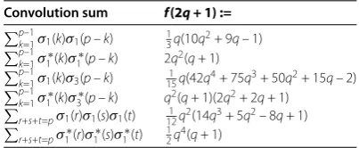
Table 2 Convolution formulas for primep= 2q+ 1

Convolution sum f(2q+ 1) := p–1

k=1σ1(k)σ1(p–k) 1₃q(10q2+ 9q– 1) p–1

k=1σ1∗(k)σ1∗(p–k) 2q2(q+ 1) p–1

k=1σ1(k)σ3(p–k) ₁₅1q(42q4+ 75q3+ 50q2+ 15q– 2) p–1

k=1σ1∗(k)σ3∗(p–k) q2(q+ 1)(2q2+ 2q+ 1)

r+s+t=pσ1(r)σ1(s)σ1(t) 121q2(14q3+ 5q2– 8q+ 1)

r+s+t=pσ1∗(r)σ1∗(s)σ1∗(t) 1 2q4(q+ 1)

Table 3 Convolution formulas

Convolution sum

A(N) :=N_k=1–1σ1(k)σ1(N–k) ₁₂1(5σ3(N) + (1 – 6N)σ1(N))

B(N) :=Nk=1–1σ1∗(k)σ1∗(N–k) 14(σ3∗(N) –Nσ1∗(N))

C(N) :=r+s+t=Nσ1(r)σ1(s)σ1(t) 1927 σ5(N) + (965 – 5 32N)σ3(N)

+ (₁₉₂1 –₁₆1N+1₈N2_)σ 1(N)

D(N) :=_r+s+t=Nσ₁∗(r)σ₁∗(s)σ₁∗(t) ₆₄1(σ₅∗(N) – 3Nσ₃∗(N) + 2N2_σ∗ 1(N))

Remark . Ifp= q+  is any odd prime, then

q

k=

σ_∗(k)σ_∗(q+  –k)≡

q

k=

σ_∗(k)σ_∗(q+  –k)

≡

r+s+t=q+

σ_∗(r)σ_∗(s)σ_∗(t)

≡ modS(q+ )

from Table .

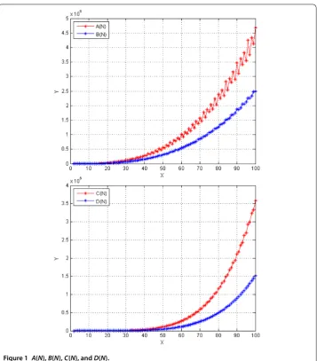
Now, we compare the values of the convolution sums in Table  [, p.]. For almost all N∈N, we find thatA(N) >B(N) andC(N) >D(N) (Figure ). As an application to Theorem ., we have the following.

Theorem . The q-seriesA(q),B(q),C(q)are connected by the differential equation,

A_{(q) =C(q) – q}dB(q)

dq + q

dA(q) dq + q

dA(q)

dq , ()

where qdB_dq(q)=∞_N=Nσ_∗(N)qN _{and q}d_A(q)

dq =

∞

N=N(N– )σ∗(N)qN.

Proof We note that

A_{(q) = }

_∞

l=

σ_∗(l)ql

_∞

m=

σ_∗(m)qm

_∞

n=

σ_∗(n)qn

=

∞

N=



l+m+n=N

σ_∗(l)σ_∗(m)σ_∗(n)

qN

=

∞

N=

Figure 1 A(N),B(N),C(N), andD(N).

from Theorem .. We note thatσ_∗(N) – Nσ_∗(N) + N_σ∗

(N) is zero forN=  andN= .

Thus the differential Eq. () follows.

Remark . We also note that from Eq. () and Eq. (), we can determine the equations

A(q)B(q) =C(q) –qdB(q)

dq ()

and

A_{(q) =B(q) –q}dA(q)

dq . ()

From () and (), Eq. () can also be deduced. Using [, ()] and (), we also get

℘ τ ,τ

= π A(q) +qdA(q) dq

where

℘(z;τ) =



z +

ω∈τ, ω=

 (z–ω) –

 ω

andτ =Z+τZ(τ∈Hthe complex upper-half plane) is a lattice andz∈C.

4 The convolution sumN_k=1–1

σ

σ

Theorem . Let N be a positive integer.And let m,n∈N∪ {}.Then we have

N–

k=

σ_∗mk; σ_∗n(N–k); = n+m–σ_∗(N; ) –Nσ_∗(N; ).

Proof From Proposition . and Eq. (), we can deduce that

N–

k=

σ_∗m_{k; σ}∗



n_{(N–k); }

= n+m N–

k=

σ(k) –σ k



σ(N–k) –σ N–k



= n+m _N–

k=

σ(k)σ(N–k) –

N–

k=

σ(k)σ

N–k



– N–

k=

σ k



σ(N–k) +

N–

k=

σ k



σ N–k



.

Now, we note that

N–

k=

σ(k)σ N–k



=

t<N/

σ(N– t)σ(t),

N–

k=

σ k



σ(N–k) =

t<N/

σ(t)σ(N– t),

N–

k=

σ k



σ

N–k



=

t<N/

σ(t)σ N

 –t

.

Therefore, the theorem follows from Eq. () and Proposition .(b).

Theorem . Let N be a positive integer and let m,n∈N∪ {}.Then we have

N–

k=

σ_∗mk; σ_∗n(N–k); 

= m_·n





σ_∗(N) –σ_∗ N 

– Nσ_∗(N) – Nσ_∗(N; ) –a(N)

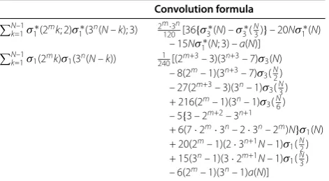
Table 4 N_k=1–1σ₁∗(2mk; 2)σ₁∗(3n(N–k); 3) andN_k=1–1σ1(2mk)σ1(3n(N–k))

Convolution formula

N–1

k=1σ1∗(2mk; 2)σ1∗(3n(N–k); 3) 2m·3n

120 [36{σ3∗(N) –σ3∗( N

3)}– 20Nσ1∗(N)

– 15Nσ₁∗(N; 3) –a(N)]

N–1

k=1σ1(2mk)σ1(3n(N–k)) 2401 [(2m+3– 3)(3n+3– 7)σ3(N)

– 8(2m– 1)(3n+3– 7)σ3(N₂)

– 27(2m+3_{– 3)(3}n_{– 1)σ} 3(N3)

+ 216(2m– 1)(3n– 1)σ3(N₆)

– 5{3 – 2m+2– 3n+1

+ 6(7_·2m_·3n_{– 2·3}n_{– 2}m_)N}σ 1(N)

+ 20(2m_{– 1)(2·3}n+1_{N– 1)σ} 1(N2)

+ 15(3n– 1)(3·2m+1N– 1)σ1(N₃)

– 6(2m_{– 1)(3}n_{– 1)a(N)]}

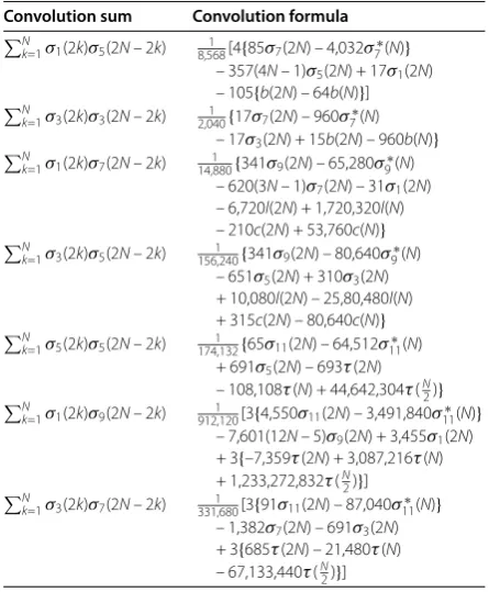
Table 5 Some convolution formulas

Convolution sum Convolution formula

N–1

k=1σ1∗(k)σ5∗(N–k) 1

408{12σ7∗(N) – 17Nσ5∗(N) + 5b(N)} N–1

k=1σ3∗(k)σ3∗(N–k) 1361 {σ7∗(N) –b(N)} N–1

k=1σ1∗(k)σ7∗(N–k) 9921 {17σ9∗(N) – 31Nσ7∗(N) + 448l(N) + 14c(N)} N–1

k=1σ3∗(k)σ5∗(N–k) 4961 {σ9∗(N) – 32l(N) –c(N)} N–1

k=1σ5∗(k)σ5∗(N–k) 1

2,764{σ11∗(N) –τ(N) + 692τ( N 2)} N–1

k=1σ1∗(k)σ9∗(N–k) 1

27,640{310σ11∗(N) – 691Nσ9∗(N) + 381τ(N) + 109,488τ( N 2)} N–1

k=1σ3∗(k)σ7∗(N–k) 1

22,112{17σ11∗(N) – 17τ(N) – 13,112τ( N 2)}

Proof We note that

N–

k=

σ_∗mk; σ_∗n(N–k); 

= m·n N–

k=

σ(k) –σ k



σ(N–k) –σ N–k



= m·n _N–

k=

σ(k)σ(N–k) –

k<N/

σ(N– k)σ(k)

–

k<N/

σ(k)σ(N– k) +

k+m=N

σ(k)σ(m)

.

Now, the theorem follows from (), Proposition .(a), (b), and Eq. ().

Remark . We can compare the two sums

N–

k=

σ_∗mk; σ_∗n(N–k); ,

N–

k=

σ

mkσ

n(N–k)

as follows (see Table ). Here we find the formula for the sumN_k=–σ(mk)σ(n(N–k))

in a similar way as in Theorem . (see [, Theorem .]).

5 Congruence relations of coefficients of certain modular-like functions

Proof We use Table  in the Appendix, and the proof of Lemma . is now similar to the

proof of Theorem ..

Remark . It is easy to observe that

N–

k=

σ_∗(k)σ_∗(N–k) =  

N–

k=

σ_∗(k)σ_∗(N–k)

whenNis odd.

As an application to the explicit evaluation of convolution sums, using Table  we prove the following theorem.

Theorem . If N is odd,then

(a) b(N)≡Nσ(N) (mod).In particularN≡ (mod),we have b(N)≡Nσ(N) (mod).

(b) b(N)≡σ(N) (mod,).In particularN≡ (mod),we have b(N)≡σ(N) (mod,).

(c) τ(N)≡σ(N) (mod,).In particularN≡ (mod),we have

τ(N)≡σ(N) (mod,,).

Proof Since the proofs of (a), (b), and (c) are similar, we only prove (c). WhenNis odd, from Table , we see that

,

N– 

k=

σ_∗(k)σ_∗(N–k) =σ(N) –τ(N). ()

SinceNis odd,k≡N–k(mod), and hence eitherkis even orN–kis even. Then, by (), σ_∗(k) = _σ∗

(k) orσ∗(N–k) = σ∗(N–k). So, in general,

τ(N)≡σ(N) (mod,).

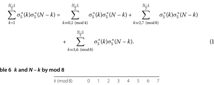
In particular, forN≡ (mod), we have Table  and

N– 

k=

σ_∗(k)σ_∗(N–k) =

N– 

k≡, (mod)

σ_∗(k)σ_∗(N–k) +

N– 

k≡, (mod)

σ_∗(k)σ_∗(N–k)

+

N– 

k≡, (mod)

σ_∗(k)σ_∗(N–k). ()

Table 6 kandN–kby mod 8

k(mod 8) 0 1 2 3 4 5 6 7

Ifn≡ (mod), then there exists a primep≡ (mod) satisfyingpi–_|nandpi_{n. Thus}

σ_∗(n) =σ_∗ n

pi–

σ_∗pi–

=σ_∗ n

pi–

 +p+p·+· · ·+p(i–)

≡ (mod). ()

Therefore, we obtain

σ_∗(k+ )σ_∗(k+ )≡σ_∗(k+ )σ_∗(k+ )

≡ mod.

Arguing in a similar manner as in (), we get

σ_∗(k+ )≡ (mod)

and

σ_∗(k+ )≡ (mod).

Therefore, we obtain

σ_∗(k+ )σ_∗(k+ )≡σ_∗(k+ )σ_∗(k+ )

≡ mod. ()

Usingσ_∗(l) = _σ∗

(l), (), and Table , we get

N– 

k=

k≡, (mod)

σ_∗(k)σ_∗(N–k)≡ (mod) ()

and

N– 

k=

k≡, (mod)

σ_∗(k)σ_∗(N–k)≡ mod. ()

Therefore, by (), (), and (), we have

τ(N)≡σ(N) (mod,,).

Remark . The same result (c) of Theorem . has been obtained by Lahiri by a different approach considering the Eisenstein series and so on (see [, (.)-(.)], [, p.]).

Corollary . Suppose that N= ,a+b is a prime number with(,,b) = .

Proof Using Mathematica ., we first findb with ≤b< , satisfying (,,

b) = . Then ifN= ,a+bis a prime number, then we find that by Theorem . (c), using Mathematica .,

τ(N)≡σ_∗(N)≡b+ ≡ (mod,)

except forb= –. Thus the corollary follows.

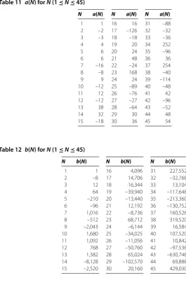
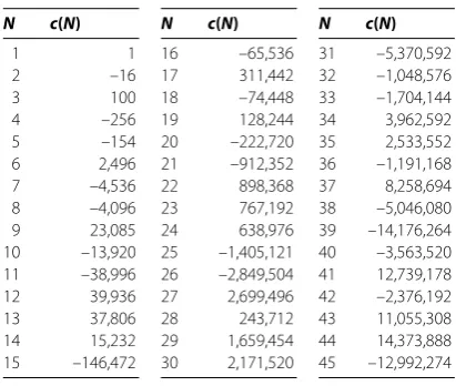
Example . Some values ofb(N),Nσ(N),σ(N),τ(N), andσ(N) are listed in Table .

Corollary . Let N∈N.Then we have Table.

In particular,if N is odd,then we have Table.

Table 7 Some values ofb(N),Nσ5(N),σ7(N),τ(N), andσ11(N)

N  3 5 7 9

b(N) 1 12 –210 1,016 –2,043

Nσ5(N) 1 732 15,630 117,656 533,637

σ7(N) 1 2,188 78,126 823,544 4,785,157

τ(N) 1 252 4,830 –16,744 –113,643

σ11(N) 1 177,148 48,828,126 1,977,326,744 31,381,236,757

Table 8 Some convolution formulas

Convolution sum Convolution formula

N

k=1σ1(2k– 1)σ5(2N– (2k– 1)) ₄₀₈1 {768σ7∗(N) + 5b(2N) – 320b(N)} N

k=1σ3(2k– 1)σ3(2N– (2k– 1)) ₁₃₆1 {64σ7∗(N) –b(2N) + 64b(N)} N

k=1σ1(2k– 1)σ7(2N– (2k– 1)) 4961 {2,176σ9∗(N) + 224d(2N) – 57,344l(N)

+ 7c(2N) – 1,792c(N)}

N

k=1σ3(2k– 1)σ5(2N– (2k– 1)) 4961 {256σ9∗(N) – 32d(2N) + 8,192l(N)

–c(2N) + 256c(N)}

N

k=1σ5(2k– 1)σ5(2N– (2k– 1)) 2,7641 {1,024σ11∗(N) –τ(2N) + 1,716τ(N)

– 708,608τ(N 2)} N

k=1σ1(2k– 1)σ9(2N– (2k– 1)) 27,6401 {317,440σ11∗(N) + 381τ(2N)

– 280,656τ(N) – 112,115,712τ(N₂)}

N

k=1σ3(2k– 1)σ7(2N– (2k– 1)) _22,1121 {17,408σ11∗(N) – 17τ(2N) + 4,296τ(N)

+ 13,426,688τ(N 2)}

Table 9 Some convolution formulas for oddN

Convolution sum Convolution formula

N

k=1σ1(2k– 1)σ5(2N– (2k– 1)) 171{32σ7(N) – 15b(N)} N

k=1σ3(2k– 1)σ3(2N– (2k– 1)) 171{8σ7(N) + 9b(N)} N

k=1σ1(2k– 1)σ7(2N– (2k– 1)) 4961 {2,176σ9(N) + 224d(2N) – 57,344l(N) + 7c(2N) – 1,792c(N)} N

k=1σ3(2k– 1)σ5(2N– (2k– 1)) ₄₉₆1 {256σ9(N) – 32d(2N) + 8,192l(N) –c(2N) + 256c(N)} N

k=1σ5(2k– 1)σ5(2N– (2k– 1)) ₆₉₁1 {256σ11(N) + 435τ(N)} N

k=1σ1(2k– 1)σ9(2N– (2k– 1)) 6911 {7,936σ11(N) – 7,245τ(N)} N

Proof Since the proofs for the convolution sums are similar, we only proveN_k=σ(k–

)σ(N– (k– )). We write

N–

k= σ∗(k)σ∗(N–k) as follows:

N–

k=

σ_∗(k)σ_∗(N–k)

= N

k=

σ_∗(k– )σ_∗N– (k– )+ N–

k=

σ_∗(k)σ_∗(N– k)

= N

k=

σ_∗(k– )σ_∗N– (k– )+  N–

k=

σ_∗(k)σ_∗(N–k) ()

by (). Also since k–  and N– (k– ) are odd, we find that

N

k=

σ_∗(k– )σ_∗N– (k– )= N

k=

σ(k– )σ

N– (k– ).

So, we obtain the formula forN_k=σ(k– )σ(N– (k– )) by () and Table . In

particular, ifNis odd, thenb(N) =b()b(N), becauseb(N) is multiplicative. Therefore

the proof is complete.

By eliminatingb(N),c(N), andl(N) in Table , we can obtain the following example.

Example . LetN∈N. Then fork= , , , we have

k–

s=

k

s+  N–

m=

σ_∗_{k–s–}(m)σ_∗_s+(N–m)

=  

σ_∗_k+(N) –Nσ_∗_k–(N).

Fork= , we refer to Eq. ().

Now we present some convolution formulas in Table .

6 Certain combinatorial convolution sum

The four basic theta functions are defined below following the notation of Whittaker and Watson [, p.]. Letτ ∈Cbe such thatIm(τ) > . Setq=eπiτ _{so that|q|< . Forz∈C,}

we define (as in [])

θ(z,q) :=  ∞

N=

(–)N–q(N–) _{sin(N– )z,}

θ(z,q) :=  ∞

N=

q(N–)_{cos(N– )z,}

θ(z,q) :=  +  ∞

N=

qNcosNz,

θ(z,q) :=  +  ∞

N=

Table 10 Some convolution formulas

Convolution sum Convolution formula

N

k=1σ1(2k)σ5(2N– 2k) _8,5681 [4{85σ7(2N) – 4,032σ7∗(N)}

– 357(4N– 1)σ5(2N) + 17σ1(2N)

– 105{b(2N) – 64b(N)}]

N

k=1σ3(2k)σ3(2N– 2k) _2,0401 {17σ7(2N) – 960σ7∗(N)

– 17σ3(2N) + 15b(2N) – 960b(N)} N

k=1σ1(2k)σ7(2N– 2k) _14,8801 {341σ9(2N) – 65,280σ9∗(N)

– 620(3N– 1)σ7(2N) – 31σ1(2N)

– 6,720l(2N) + 1,720,320l(N) – 210c(2N) + 53,760c(N)}

N

k=1σ3(2k)σ5(2N– 2k) 156,2401 {341σ9(2N) – 80,640σ9∗(N)

– 651σ5(2N) + 310σ3(2N)

+ 10,080l(2N) – 25,80,480l(N) + 315c(2N) – 80,640c(N)}

N

k=1σ5(2k)σ5(2N– 2k) 174,1321 {65σ11(2N) – 64,512σ11∗(N)

+ 691σ5(2N) – 693τ(2N)

– 108,108τ(N) + 44,642,304τ(N 2)} N

k=1σ1(2k)σ9(2N– 2k) _912,1201 [3{4,550σ11(2N) – 3,491,840σ11∗(N)}

– 7,601(12N– 5)σ9(2N) + 3,455σ1(2N)

+ 3{–7,359τ(2N) + 3,087,216τ(N) + 1,233,272,832τ(N₂)}]

N

k=1σ3(2k)σ7(2N– 2k) 331,6801 [3{91σ11(2N) – 87,040σ11∗(N)}

– 1,382σ7(2N) – 691σ3(2N)

+ 3{685τ(2N) – 21,480τ(N) – 67,133,440τ(N₂)}]

Jacobi (see [, ]) proved that

θ(,q)θ(,q)θ(z,q)

θ(z,q)

= 

∞

m= qm+

 –qm+sin(m+ )z ()

and

θ_(,q)θ

(,q)θ(z,q)

θ_(z,q) = 

∞

m= mqm

 –qm( –cosmz). ()

From () and (), we deduce that

∞

m= mqm

 –qm( –cosmz) = 

_∞

m= qm+

 –qm+sin(m+ )z



. ()

Equating coefficients ofqN(N∈N) on the left- and right-hand sides of () (see [, p.]), then we obtain the arithmetical equality involving the trigonometric functions

m∈N m|N

N m odd

m( –cosmz) =

(a,b,x,y)∈N

ax+by=N a,b,x,yodd

cos(a–b)z–cos(a+b)z. ()

If we expand each cosine in powers ofzusing

 –cosz=

∞

k=

(–)k–z

k

and equate coefficients of z__kk_! (k∈N), then we obtain

m∈N m|N

N m odd

kmk+=

(a,b,x,y)∈N

ax+by=N a,b,x,yodd

(a+b)k– (a–b)k, k,N∈N. ()

A generalized Besge formula due to Liouville is as follows.

Proposition .(See [, Theorem .]) Let k∈Nand N∈N,where k,N≥.Then we have

k–

s=

k

s+  N–

m=

σk–s–(m)σs+(N–m)

=k+ 

k+ σk+(N) +

k

–N

σk–(N) +

 k+ 

k

j=

k+  j

Bjσk+–j(N),

where Bjis thejth Bernoulli number.

Letσs,oo(N) :=

d|N dodd

n dodd

ds. Now we prove the following lemma.

Lemma . We have

k–

s=

k

s+  N–

m=

σk–s–,oo(m)σs+,oo(N–m) =  σ

∗ k+(N).

Proof First we consider

(a,b,x,y)∈N_,

ax+by=N,

a≡b≡x≡y≡mod

(a+b)k– (a–b)k

=

(a,b,x,y)∈N,

ax+by=N,

a,b,x,yodd

_k

r=

k r

ak–rbr–

k

r=

k r

(–)rak–rbr

= 

(a,b,x,y)∈N_,

ax+by=N,

a,b,x,yodd k

r=,

rodd

k r

ak–rbr=  k–

s=

k

s+ 

(a,b,x,y)∈N_,

ax+by=N,

a,b,x,yodd

ak–s–bs+

=  k–

s=

k

s+  N–

m=

a|m,

aodd,

m a odd

ak–s–

b|N–m,

bodd, N–m

b odd

bs+

=  k–

s=

k

s+  N–

m=

Now the right-hand side of () is

d∈N,

d|N,

dN_

kdk+= k d|N

dk+–

d|N dk+

= k

σk+(N) –σk+ N



= kσ_∗_k+(N) =  σ

∗ k+(N)

by (). Therefore we obtain

k–

s=

k

s+  N–

m=

σk–s–,oo(m)σs+,oo(N–m) =  σ

∗

k+(N).

As a consequence of Proposition . and Lemma ., we have the following.

Theorem .

k–

s=

k

s+  N–

m=

σk–s–(m)σs+(N– m)

=k+ 

k+ σk+(N) –  σ

∗

k+(N) + k

– N

σk–(N)

+  k+ 

k

j=

k+  j

Bjσk+–j(N),

where Bjis thejth Bernoulli number.

Proof From Proposition ., we get

k–

s=

k

s+  N–

m=

σk–s–(m)σs+(N–m)

=k+ 

k+ σk+(N) +

k

– N

σk–(N)

+  k+ 

k

j=

k+  j

Bjσk+–j(N) ()

by replacingN→N. From Lemma . we know that

k–

s=

k

s+  N–

m=

σk–s–,oo(m)σs+,oo(N–m) =  σ

∗ k+(N)

= k–

s=

k

s+ 

N

m=

σk–s–(m– )σs+(N– m+ ). ()

Remark . It is well known that

B= , B= –



, B= 

, Bj+=  (j≥), . . . .

In Proposition ., takingN= , we obtain

 =k+  k+ +

k

– 

+  k+ 

k

j=

k+  j

Bj

= 

k+ +   + k –  +  k+ 

k

j=

k+  j

Bj

=  k+ 

k+  

B+

 k+ 

k+  

B+

 k+ 

k+  

B

+  k+ 

k

j=

k+ 

j

Bj

and this implies the well-known identity involving the Bernoulli numbersBj

 k+ 

k

j=

k+ 

j

Bj= . ()

In Theorem ., takingN= , we obtain

 =  k+ +

 

 + k++ k –  – 

 + k–– ·

k+

+  k+ 

k

j=

k+  j

Bk+–j·

 + k+–j.

Then we have

 =  k+ +

  + k –  +  k+ 

k

j=

k+  j

Bk+–j

+  k+ 

k+_{+ }k_{– }k–₊k

·

k–

+  k+ 

k

j=

k+  j

Bk+–jk+–j–  – k–– k–. ()

Using () and (), we get

 =  k+ 

k+  

k+–  k+ 

k+  

k+– – 

+  k+ 

k+  

k+–+  k+ 

k

j=

k+ 

j