Development of a High Resolution Multiscale Modeling and Prediction System for Bay of Bengal, Part II: An Application to October 2008

http://dx.doi.org/10.4236/ojms.2016.61012

How to cite this paper: Chakraborty, A. and Gangopadhyay, A. (2016) Development of a High-Resolution Multiscale Mod-eling and Prediction System for Bay of Bengal, Part II: An Application to October 2008. Open Journal of Marine Science, 6, 125-144. http://dx.doi.org/10.4236/ojms.2016.61012

Development of a High-Resolution

Multiscale Modeling and Prediction

System for Bay of Bengal, Part II: An

Application to October 2008

Arun Chakraborty1*_{, Avijit Gangopadhyay}1,2,3

1_{Centre for Oceans, Rivers, Atmosphere and Land Sciences (CORAL), Indian Institute of Technology Kharagpur,}

Kharagpur, India

2_{School of Earth, Ocean and Climate Sciences, Indian Institute of Technology Bhubaneswar, Bhubaneswar, India} 3_{School for Marine Science and Technology, University of Massachusetts, Dartmouth, USA}

Received 2 December 2015; accepted 26 January 2016; published 29 January 2016

Copyright © 2016 by authors and Scientific Research Publishing Inc.

This work is licensed under the Creative Commons Attribution International License (CC BY).

http://creativecommons.org/licenses/by/4.0/

Abstract

A high-resolution (10 km × 10 km) multiscale ocean modeling system was developed for the Bay of Bengal (BOB) region for short-term ocean hindcasts/forecasts. A physical validation of this system that was based on climatological initialization and short-term simulations was presented in Part I of this series of studies. Realistic structures for prevalent eddies, fronts and gyres were reasonably reproduced and validated for three individual months (February, June and October). In this study, we present an application and synoptic validation of the system for October 2008 in a hindcast mode. The system is based on the Regional Ocean Modeling System (ROMS), which assimilates sa-tellite and in-situ measurements within the background climatology using an objective analysis to produce the synoptic initial condition for the model and/or to produce an estimation of the cur-rent ocean state. A meteorological forecast is then input into this synoptic three-dimensional ocean model to produce the ocean hindcast/forecast. The high-density Array for Real-time Geo-tropic Oceanography (ARGO) observations, and the Tropical Rain Measuring Mission (TRMM) sa-tellite’s microwave imager (TMI) passes during the beginning of the month of October 2008, pro-vided a unique opportunity for the system to assimilate these in-situ observations at initialization. Then, the ARGO and TMI observations during the later part of October 2008 were used for the sta-tistical validation of the system’s fidelity. The validation shows that the hindcast/forecast system can reasonably predict the ocean currents, temperature and salinity. The forecast error increases as the forecast time window increases, although the system has a reasonable predictability for up to seven to ten days. The assimilation of both in-situ ARGO and satellite data at initialization

A. Chakraborty, A. Gangopadhyay

duced better hindcasts/forecasts.

Keywords

ARGO, TMI, ROMS, Simulation

1. Introduction

Operational ocean forecast models are now available on all scales, from global to local. Typically, such models are initialized by climatological data when needed or, if the direct measurements of oceanic parameters are available for the region of interest, by melding climatology with observations. For applications in fisheries management and for naval operations, fine-resolution ocean forecasts are frequently required for limited regions.

The Bay of Bengal is a land-locked region (Figure 1(a))with a semi-annually reversing wind system that causes a semi-annually reversing surface circulation. Severe tropical cyclones that are generated during the spring (April-May) and fall (October) cause large-scale flooding and destruction along the coast; such a region requires a forecasting system. However, because of the scarcity of in-situ data, many mesoscale features are not well understood, and no prediction system is available for this region. Thus, for the first time, a high-resolution multiscale ocean prediction system was developed using ROMS [1][2] for the BOB basin (Figure 1(b)). This ocean forecasting system is intended to produce a daily, short-term (one week to ten day) forecast of the mesos-cale ocean current, temperature, salinity and sea-level variation.

The first step in generating a prediction system is to validate the system and to develop phenomenological features in a realistic manner. The shapes, sizes and occurrences of major features should be reproduced in a realistic and statistical manner. In our Part I paper [3], we discussed different multiscale features from climatol-ogy-based simulations over a 30-day period for three periods: February for winter, June for summer, and Octo-ber for fall.

To make the forecasts as close as possible to reality, the models are driven by synoptic atmospheric forcing fields and by the assimilation of real-time observations, which may consist of remotely sensed data and in-situ

measurements. We conducted experiments to assess the forecast capability by assimilating TMI and ARGO data sets for October 4-6, 2008 with Levitus 0.25˚ × 0.25˚ climatology [4][5] and by applying surface forcing. The prediction system methodology and comparison of the ocean hindcasts/forecasts to the synoptic simulation are discussed in detail in this paper. Section 2 describes the prevalent features in October; Section 3 describes the TMI and ARGO data sets and model domain; Section 4 describes the experimental setup; Section 5 provides the evolution of the synoptic simulation and validation; and Section 6 provides the summary and conclusions.

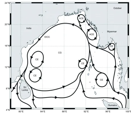
2. Prevalent Features in the BOB Region during October

A schematic presentation of the oceanographic features in the BOB region during October is shown inFigure 2. This representation is required to validate the regional oceanographic features with respect to the model simula-tions. A list of relevant studies that were used to identify the features is provided inTable 1. In October, the northeast monsoon has just started, and the surface circulation is dominated by a basin-scale cyclonic gyre (CG) with mesoscale anticyclonic eddies (AE) at 91˚E, 21˚N and 93˚E, 18˚N and cyclonic eddies (CE) at 97˚E, 16˚N; 95˚E, 10˚N; 83˚E, 11˚N; 83˚E, 13˚N; and 91˚E, 12.5˚N. The surface circulation shows a well-defined boundary current along the Indian coast, known as the East India Coastal Current (EICC), which moves toward the equa-tor [6]. The Indian Ocean water enters the BOB at around 90˚E. During October, warm water enters the Anda-man Sea through the Malacca Strait and may originate from the South China Sea [6].

(a)

(b)

A. Chakraborty, A. Gangopadhyay

Figure 2. Schematic diagram of the prevalent features during October that were derived from different observational studies. The EICC and basin-scale cyclonic gyre are the broad-scale features of the basin during October. There are also a few me-soscale eddies during this time.

Table 1. List of relevant studies used to identify the features.

Features Relevant studies

EICC [3][6][8] [22]-[26]

Basin scale CG [3][7][8][10][26]

Anti-cyclonic gyre at head Bay of Bengal [3][10][27]-[29]

and then moves northward to join with the EICC at 20˚N to complete a basin-scale cyclonic gyre in the Bay of Bengal [10]. There are anticyclonic eddies near the Myanmar coast that cause both the eastern boundary and the western boundary currents of the North Bay to move southward. A portion of the Malacca Strait flow moves northward along the eastern boundary and then meets the basin-wide CG around 15˚N.

another feature during October [9]. Two anti-cyclonic eddies (95˚E, 12˚N; 97˚E, 7˚N) in the Andaman Sea are

also features of this level. In a deeper zone, the western Bay is covered with a cyclonic gyre with currents fol-lowing the boundary, and the Andaman Sea is covered with an anticyclonic gyre.

3. Data, Model and Methodology

The ROMS used in our study [3] is a free-surface, hydrostatic, primitive equation ocean model [2] with a stretched terrain-following S-coordinate system. The primitive equations are written using boundary-fitted, or-thogonal, curvilinear coordinates on a staggered Arakawa C grid [1]. This regional model was configured for the BOB region (4˚N - 24˚N, 79˚E - 100˚E) with 256 × 249 grid points in the horizontal surface approximately 10 km resolution. The northern, eastern and major parts of the western boundaries were closed, while the southern boundary was open. On the open boundary, the temperature and salinity values were relaxed to the Levitus monthly climatology. The vertical turbulent mixing was based on the K-profile parameterization (KPP) vertical mixing scheme. The model consists of 32 S-coordinate layers in the vertical, and the bottom topography was based on the Earth Topography Two-Minute digital terrain model (ETOPO2) data (Figure 1(b)).

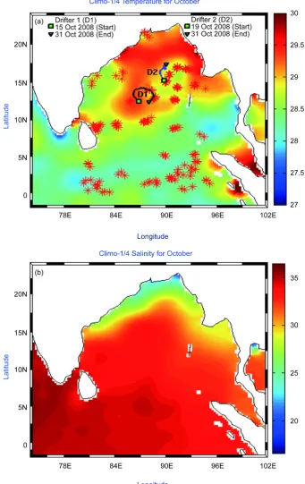
The following data were used to create the initial fields: the Levitus temperature and salinity climatology fields on the 0.25˚ × 0.25˚ [4][5] grid (Figure 3(a),Figure 3(b)); the ocean observational ARGO data sets for the month of October 2008 (overlaid in Figure 3(a)); and the SST measured by the TMI on a 0.25˚ × 0.25˚ grid

that passed over the BOB region during October 4-6, 2008. The TMI data was obtained from

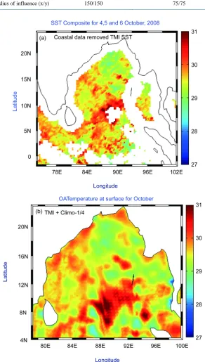
ftp://ftp.ssmi.com/tmi/bmaps_v04/. Because the TMI composite values are high near the coast and are not

realis-tic [11], the temperature data near the coast were removed (Figure 4(a)). These temperature data were then sub-sampled for every grid point to construct the synthetic temperature profile (Tsyn) using Equation (1) as follows:

(

)

( )

( )

(

)

( )

syn TMI b b

T x y z =_T x y −T x y _ ϕ x y z +T x y ≤ ≤z H (1)

(

)

(

_{( )}

)

_{( )}

( )

b

s b

T x y z T x y

x y z z H

T x y T x y

ϕ =  −  ≤ ≤

 − 

  (2)

where ϕ(x, y, z) is the non-dimensional structiure function, Ts(x, y) is the surface temperature from Levitus

Cli-maotology, Tb(x, y) is the Levitus temperature at depth H and TTMI(x, y) is the TMI SST.

To prepare the initial field on the model grid points, an objective analysis (OA) procedure [12]-[14] was per-formed with the synthetic profiles of temperature and Levitus salinity profiles using the Levitus October clima-tology as the background. OA has the advantage over the direct interpolation from the Levitus grid of modeling the grid by keeping the dynamical feature information intact [13] and melding the satellite and in-situ data in an optimal statistical way. The multiscale OA parameters used are given inTable 2.

A. Chakraborty, A. Gangopadhyay

Table 2.Multiscale OA parameters.

OA parameters Climatology large-scale (km) Mesoscale (10 km resolution) (km)

Zero-crossing (x/y) 300/300 150/150

Radius of influence (x/y) 150/150 75/75

Figure 4. (a) Composite picture of the sea surface temperature derived from the TMI that passed over the Bay of Bengal on October 4-6, 2008. The coastal temperature was removed because the TMI satellite picture showed hotter regions along the coast; (b) The model initial field of temperature for the month of October 2008 at the surface derived from OA fields for

A. Chakraborty, A. Gangopadhyay

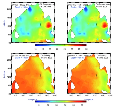
Figure 5. The model initial field of temperature for the month of October 2008 at the depth of 100 m derived from OA fields is shown for (a) Exp-2and (b) Exp-3. The model initial field of salinity for the month of October 2008 at the depth of 100 m derived from OA fields is shown for (c) Exp-2and (d) Exp-3. The impact of ARGO was seen in Exp-3at this depth.

4. Experimental Setup

The following three short-term (30 day) model experiments were conducted, using October 4-6, 2008 ARGO and satellite data-based OA as initial conditions to access the impact of TMI and ARGO data. These experi-ments were performed as follows: Exp-1, simulation with the Climo-1/4data as initial fields; Exp-2, simulation with the TMI-Climo-1/4data as initial fields; and Exp-3, simulation with the ARGO-TMI-Climo-1/4data as ini-tial fields. The model was forced with COADS (Comprehensive Ocean Atmosphere Data Set) October clima-tology-based surface forcing.

synoptic short-term simulations at initialization. The initial geostrophic velocity was computed from the temper-ature and salinity by the OA methodology [13] described above. Similar initialization methodology and their in-ternal adjustment procedures were described by [15][17]-[19].

5. Evaluation against Climatology Simulation

The time evolutions of kinetic energy for the different simulation experiments are shown in Figure 6. The ki-netic energy slowly increased with the time of integration in all simulations. The kiki-netic energy for the TMI si-mulation (Exp-2) was larger than that for the climatology simulation (Exp-1) and less than that for the TMI plus ARGO simulation (Exp-3). It can be inferred from this figure that both TMI and ARGO introduced many me-soscale features to the climatology data, and as a result, the kinetic energy increased.

5.1. Circulation Features

5.1.1. Surface

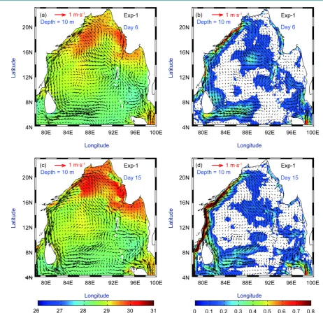
The surface circulations for Exp-1, Exp-2and Exp-3are shown inFigure 7, Figure 8 and Figure 9, respectively. The surface circulation features for Exp-2and Exp-3(Figure 8 andFigure 9) were much more prominent than those in Exp-1(Figure 7), with few additional features. The development of a well-defined coast following the East India Coastal Current (EICC), which moves toward the equator [6], was observed in all the experiments from day 6 to day 15 of the model integrations. The bifurcation of the EICC at the northern tip of Sri Lanka and the flow of the branches were well approximated by all of the model simulations. The basin-scale cyclonic gyre in the Bay of Bengal could be seen in the model simulation experiments from day six (Figure 7(a),Figure 8(a),

Figure 9(a)). This gyre was more organized, and its boundary current strength (Figure 7(b),Figure 8(b), Fig-ure 9(b)) was comparable with observations [10] for day 15 of the model simulation experiments (Figure 7(c),

Figure 8(c), Figure 9(c)). The flow to the Andaman Sea region from the South China Sea via the Malacca Strait

[6], which was observed in Exp-1(Figure 7(c)), was also seen in the Exp-2(Figure 8(c)) and Exp-3(Figure 9(c)) model simulations. The last two simulation experiments demonstrated that the penetration of this flow to the Bay of Bengal was eastward and the flow to the Indian Ocean was southward from the northern tip of Suma-tra Island (Figure 8(d), Figure 9(d)). The surface flow through the Palk Strait to the Arabian Sea from the Bay of Bengal was seen for all of the model simulations. The Anticyclonic Gyre (AG) in the northeastern side of the head bay (93˚E, 18˚N), which triggers the southward movement of both eastern boundary and western boundary currents, was prominent from day 6 to day 15 of the model integrations for Exp-2(Figures 8(a)-(d)) and Exp-3 (Figures 9(a)-(d)). The eastern boundary current above 16˚N was strong on day 15 for the Exp-2(Figures 8(c),

Figure 8(d)) and Exp-3(Figure 9(c),Figure 9(d)) model simulation experiments. The mesoscale eddies were prominent in the model simulations from day six of the model integration (Figure 7(a), Figure 8(a),Figure 9(a)). The mesoscale anticyclonic eddies around the centers at 91˚E, 21˚N and 93˚E, 18˚N and cyclonic eddies

A. Chakraborty, A. Gangopadhyay

Figure 7. (a) Model-simulated currents (vectors) with temperature (colored for Exp-1at the depth of 10 m for day six; (b) Model-simulated currents (vectors) with magnitude (color shaded) for Exp-1at the depth of 10 m for day six; (c) Model-si- mulated currents (vectors) with temperature (color shaded) for Exp-1at the depth of 10 m for day 15; (d) Model-simulated currents (vectors) with magnitude (colored) for Exp-1at the depth of 10 m for day 15.

around the centers at 97˚E, 16˚N; 95˚E, 10˚N; 83˚E, 11˚N; 83˚E, 13˚N; and 91˚E, 12.5˚N were apparent in all three simulation experiments (Figure 7(c),Figure 8(c), Figure 9(c)).

Figure 8. (a) Model-simulated currents (vectors) with temperature (colored) for Exp-2at the depth of 10 m for day six; (b) Model-simulated currents (vectors) with magnitude (colored) for Exp-2at the depth of 10 m for day six; (c) Model-simulated currents (vectors) with temperature (colored) for Exp-2at the depth of 10 m for day 15; (d) Model-simulated currents (vec-tors) with magnitude (colored) for Exp-2at the depth of 10 m for day 15.

5.1.2. Subsurface

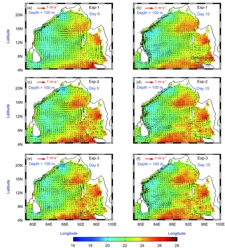
The basin-scale cyclonic gyre with southward-flowing EICC that is observed at the surface was also seen at the subsurface depth (Figures 10(a)-(f)), but it was smaller in size. This gyre was observed in the climatology-based simulation, Exp-1 (Figure 10(a), Figure 10(b)), and also with the TMI and ARGO simulation experiments,

Exp-2and Exp-3(Figure 10(b),Figure 10(c) and Figure 10(d), Figure 10(f)). The features were more promi-nent on day 15 (Figure 10(b), Figure 10(d) & Figure 10(f)) of the model simulation experiments compared to day 6 (Figure 10(a), Figure 10(c) & Figure 10(e)). The cyclonic eddies (86.5˚E, 19˚N; 82.5˚E, 14˚N; 79.5˚E,

5˚N; 83˚E, 10˚N) on the western side of the basin and anticyclonic eddies (97˚E, 7˚N; 95˚E, 12˚N; 91˚E, 17˚N) on the eastern side of the basin were observed for all three simulation experiments (Figure 10(b), Figure 10(d)

& Figure 10(f)). All of these circulation features were distinct and strong for Exp-2(Figure 10(d)) and Exp-3 (Figure 10(f)) compared to Exp-1(Figure 10(b)). The prominent anti-cyclonic eddies at 95˚E, 12˚N and 97˚E,

A. Chakraborty, A. Gangopadhyay

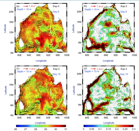
Figure 9. (a) Model-simulated currents (vectors) with temperature (colored) for Exp-3at the depth of 10 m for day six; (b) Model-simulated currents (vectors) with magnitude (colored) for Exp-3at the depth of 10 m for day six; (c) Model-simulated currents (vectors) with temperature (colored) for Exp-3at the depth of 10 m for day 15; (d) Model-simulated currents (vec-tors) with magnitude (colored) for Exp-3at the depth of 10 m for day 15.

western side of the basin, but several extra features were observed on the eastern side of the basin. These were the small cyclonic gyres with centers at 93˚E, 5˚N and 97˚E, 11˚N in Exp-2(Figure 10(d)) and Exp-3(Figure 10(f)).

These gyres result from the impact of TMI and ARGO at the subsurface because they were not observed in the climatology-based simulation. The western side of the basin is colder than the eastern side at the subsurface, which was seen from these simulation experiments (Figure 10(b), Figure 10(d) & Figure 10(f)). Other basic structures at this depth remained the same for all the simulation experiments, but the cyclonic gyres at 86.5˚E, 19˚N, at 82.5˚E, 15˚N and at 83˚E, 10˚N were more prominent in Exp-2(Figure 10(d)) and Exp-3(Figure 10(f)) than in Exp-1(Figure 10(b)). The strong southward EICC with this CG makes this region a zone of upwelling, and as a result, this region is cold.

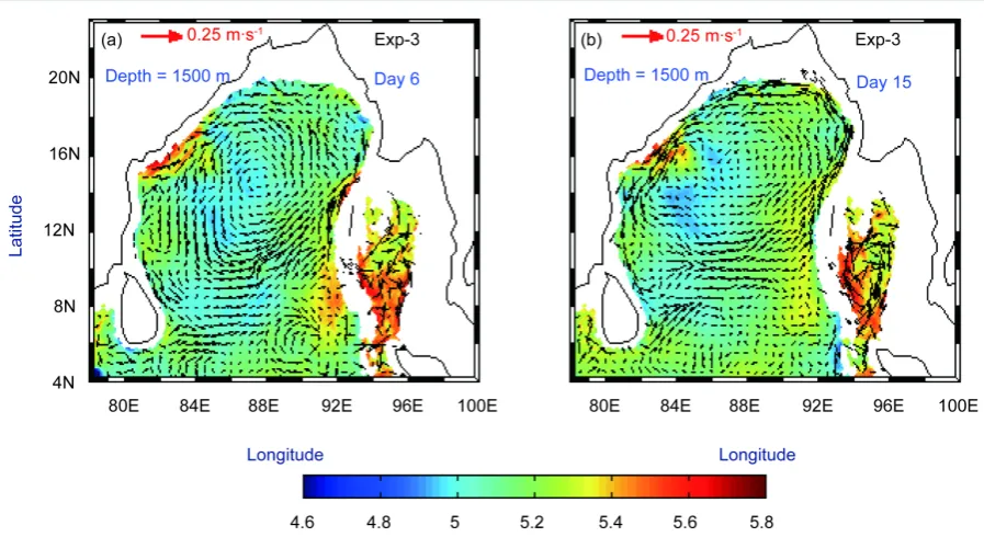
5.1.3. Deep Ocean

Figure 10. Model-simulated currents (vectors) with temperature (colored) at the depth of 100 m for (a) day 6 for Exp-1, (b) day 15 for Exp-1, (c) day 6 for Exp-2, (d) day 15 for Exp-2, (e) day 6 for Exp-3and (f) day 15 for Exp-3.

A. Chakraborty, A. Gangopadhyay

Figure 11. Model-simulated currents (vectors) with temperature (colored) at the depth of 1500 m for (a) day 6 for Exp-3and (b) day 15 for Exp-3.

5.2. Mass Transport

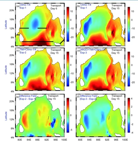
The vertically integrated mass transports for the model experiments are shown in Figures 12(a)-(d). It is evident from these figures that the BOB region was dominated by a basin-wide large cyclonic gyre with its center lo-cated at 84˚E, 14˚N. The CG was observed on day 6 (Figure 12(a)), but the strong EICC was observed on day 15 of the model simulation (Figures 12(b)-(d)) when the center of the maximum circulation of this CG shifted toward the western boundary of the basin. A small but strong AE in the Andaman Sea was observed in the mod-el simulation results (Figures 12(b)-(d)). The overall circulation in the vertical integrated volume transport for the October simulation showed two opposite gyres in the basin across a line drawn from the southwest region of Sri Lanka to the south of the Myanmar region (Figures 12(b)-(d)). The formation of different mesoscale eddies at different locations was also observed. The different fields of transport on day 15 of the model simulations showed that Exp-2enhanced the transport near the western boundary more than Exp-1(Figure 12(e)), and Exp-3 enhanced the overall transport over the basin more than Exp-2(Figure 12(f)).

The quantitative estimate of the volume transported in the upper 1000 m was computed across different sec-tions and is shown in Table 3. The northward volumes transported at 12˚N between 88˚E to 92˚E for Exp-1,

Exp-2and Exp-3were 5.34 Sv, 5.47 Sv and 6.26 Sv, respectively. [10] showed that the northward vertically in-tegrated volume transported in the upper 1000 m along the same section is 6 Sv, which is close to the volume estimated in Exp-3. At 6˚N between 80˚E to 99˚E, the volumes transported southward were 14.58 Sv, 14.65 Sv

and 14.81 Sv for Exp-1, Exp-2and Exp-3, respectively. [20] showed that the volume transport for the above sec-tion is 10 Sv, while it was reported as 16 Sv by [21]. The vertically integrated volume transport along the Palk Strait was southward, and it was small (0.67 Sv) for Exp-1, but the value increased to 1.06 Sv for Exp-2and 1.08 Sv for Exp-3. Similarly, the Malacca Strait inflow increased in the experiments, but the difference among expe-riments was decreased; it was 2.01 Sv for Exp-1, 2.03 for Exp-2 and 2.04 for Exp-3. The magnitude of the transport increased in the model simulation when ARGO and satellite observations were included in the initial conditions. The transport values along the sections were comparable to the earlier observational studies [10][20] [21].

5.3. Comparison with Observations

Figure 12. Model-simulated vertically integrated mass transport (Sv: 1 Sv = 106 m3/s) for (a) day 6 for Exp-1, (b) day 15 for

Exp-1, (c) day 6 for Exp-2, (d) day 15 for Exp-3, (e) difference fields (Exp-2- Exp-1) for day 15 of the simulation and (f) difference fields (Exp-3- Exp-2) for day 15 of the simulation. Black solid lines in (a) indicate the sections along which transport values were calculated.

Table 3.Transport through the different sections.

Sections

Transports values (Sv) of theexperiments

Observational Evidences

Exp-1 Exp-2 Exp-3

88˚E - 92˚E, 12˚N 5.34 5.47 6.26 6 Sv [10]

Creek Channel, 9˚N −0.67 −1.06 −1.08 - Malacca Strait 98˚E, 5˚N to 100˚E, 7˚N 2.01 2.03 2.04 -

80˚E - 95˚E, 6˚N −14.58 −14.65 −14.81 −16 Sv _{−10 Sv} [21]

[20]

A. Chakraborty, A. Gangopadhyay

2008 and ended on October 31, 2008, and drifter D2 started on October 19, 2008 and ended on October 31, 2008 (Figure 1(a)).

5.3.1. Comparison with ARGO

The model simulations for Exp-2were carried out with October 4-6 ARGO data-based OA as the initial condi-tions, and Exp-3was carried out with October 4-6 ARGO and TMI satellite data-based OA as the initial condi-tions. The model validation was performed by comparing the ARGO profiles available from October 10-31 with the model-simulated profiles from day 5 to day 31 in the ARGO locations. Because of the different characteris-tics of the eastern and western BOB [3], the comparisons are shown separately for the two parts of the basin. Although the comparison was performed for all the available profiles, only profiles for October 10, 15 and 20, 2008 are shown with the profiles of day 5, day 10 and day 15 of the model simulation experiments (Exp-1,

Exp-2and Exp-3) in Figure 13(a)for the western BOB and Figure 13(b)for the eastern BOB. The model per-formed well because almost all of the profiles were comparable with the observations (Figure 13(a), Figure 13(b)). It was also observed from these profiles that Exp-2was better than Exp-1, and Exp-3was better than

Exp-2. In the mixed layer, the temperature was slightly lower for the model simulations than for the ARGO pro-files (Figure 13(a), Figure 13(b)). It was observed that in the eastern side of the basin (Figure 13(b)) for the model simulation, the thermocline deepened, whereas in the western side of the basin (Figure 13(a)), the ther-mocline shifted upward compared to the ARGO profiles. The root mean square error (RMSE) of the simulation

Figure 13. Vertical profiles at ARGO locations for October 2008 with the model experiments [Exp-1(red), Exp-2(blue),

experiments for the available profiles was calculated based on ARGO observations. These RSME vertical pro-files for the simulation experiments (Exp-1, Exp-2and Exp-3) for the western BOB and the eastern BOB are shown in Figure 13(c)and Figure 13(d), respectively. It was observed from these figures that Exp-2was better than Exp-1,while Exp-3was better than the other two experiments. In the thermocline zone, the errors were larger than those for the surface and bottom regions (Figure 13(c), Figure 13(d)). The overall error at the sur-face was approximately 0.5˚C, and in the deeper zone it was approximately 0.25˚C for both the western (Figure 13(c)) and the eastern (Figure 13(d)) regions of the BOB. In the thermocline region, the error was between 0.5˚C and 2.4˚C for the western BOB (Figure 13(c)) and between about 0.5˚C and 1.8˚C for the eastern BOB

(Figure 13(d)). The percentage error at the surface, the thermocline zone and the deeper layer was about 1.6%, 11% and 2%, respectively, for the model experiments.

5.3.2. Comparison with Drifters

The model-simulated profiles were also compared between the two drifter locations that started on October 15 and 19, 2008 and days 20 and 24 of the model simulation (Figure 14(a), Figure 14(b)). We did not have drifters during the first week of simulation. The comparisons presented here are for the second and third week of the simulation, when the use of TMI and ARGO from October 4-6 was curtailed for days 19 - 30, when the drifters were collecting data. This leads to an insignificant difference between Exp-2and Exp-3for these days. Although the magnitudes were different for the simulation experiments compared to the drifters, the nature of the varia-tions was well captured by the model. The difference was smallest for Exp-3and largest for Exp-1, which indi-cates that the incorporation of ARGO and satellite data in the initial fields improved the model simulation re-sults.

6. Summary and Conclusions

A high-resolution ocean multiscale prediction system was developed for the BOB region. The system first assi-milates the in-situ observations and satellite observational data to create the synoptic initial fields in terms of the objective analysis (OA), and then the dynamical model of the ocean gives the ocean state forecast with the ap-plied meteorological forcing. The climatology-based simulations using this high-resolution multiscale prediction

A. Chakraborty, A. Gangopadhyay

Figure 15. Schematic diagram of the BOB features during October 2008 from the model simulation. More features were ob-served on the eastern boundary during October 2008 compared to the climatological features seen inFigure 2.

system for the months of February, June and October demonstrated the capability of this system to produce the current climatological systems, gyres and mesoscale eddies, which are reported in Part I [3]. The model hind-casts for the month of October 2008 were verified here.

The inclusions of satellite data (TMI) and ARGO with TMI increased the magnitude of the boundary currents and clarified different mesoscale structures compared to the climatology-based simulations. At the surface, in addition to the EICC, basin-scale gyre, anticyclonic eddies (91˚E, 21˚N; 93˚E, 18˚N; 97˚E, 11˚N; 99˚E, 6˚N) and cyclonic eddies (97˚E, 16˚N; 95˚E, 10˚N; 83˚E, 11˚N; 83˚E, 13˚N; 91˚E, 12.5˚N; 97˚E, 9˚N) were observed in

Exp-2and Exp-3. Of these eddies, the cyclonic eddy at 97˚E, 9˚N and the anticyclonic eddies (97˚E, 11˚N; 99˚E,

The quantitative estimates of the volume transport in the upper 1000 m across different sections were compa-rable with observational studies. The model with ARGO profiles performed well for October 10, 15, and 20 of 2008, and almost all of the profiles were comparable with the observations. In the mixed layer, the model tem-perature was slightly lower (less than 0.4˚C) for several locations than it was in the ARGO profiles. The vertical profile of RMSE for Exp-3was better than that in the Exp-2and Exp-1simulation experiments. In the thermoc-line zone, the errors were larger compared to those in the surface and bottom regions. The overall error was ~0.5˚C at the surface and ~0.25˚C in the deeper zone, but in the thermocline zone, it was slightly higher (0.5˚C< RMSE < 2.4˚C) for the BOB. The percentage error at the surface was about 1.6%; at the thermocline zone, it reached a maximum of ~11% and in the deeper layer it was ~2% for the model experiments.

The modeling system presented produced many mesoscale features that are not present in the climatology- based simulation due to the inclusion of satellite and in-situ observations at initialization. This is schematically captured and presented inFigure 15. The simulation of clear and distinct features as well as their proper place-ment at initialization provides a strong basis for utilizing this methodology for short-term prediction in this data- sparse region. As presented here, and considered together with Part I of the climatology-based simulations, this modeling system is now ready to be used for semi-operational experimental forecasting with a week to two weeks of expected predictability.

Acknowledgements

The authors also gratefully acknowledge the financial support given by the Earth System Science Organization (ESSO)—Indian National Centre for Ocean Information Services (INCOIS), Ministry of Earth Sciences, and Government of India to conduct this research. We wish to thank Dr. M. Ravichandran and his group at INCOIS for making the TMI and ARGO data available for this project. We are thankful to Dr. Andre Schmidt, Dr. Ayan H. Chaudhuri and Ms. Carolina Nobre for their help and support during the study. We are also grateful to Mr. Frank Smith for his editorial help.

References

[1] Hedstorm, K.S. (1997) User’s Manual for an S-Coordinate Primitive Equation Ocean Circulation Model (SCRUM) Version 3.0. Institute of Marine and Coastal Sciences, Rutgers University, 116 p.

[2] Haidvogel, D.B., Arango, H.G., Hedstrom, K., Beckmann, A., Malanotte-Rizzoli, P. and Shchepetkin, A.F. (2000) Model Evaluation Experiments in the North Atlantic Basin: Simulations in Nonlinear Terrain-Following Coordinates.

Dynamics of Atmospheres and Oceans, 32, 239-281. http://dx.doi.org/10.1016/s0377-0265(00)00049-x

[3] Chakraborty, A. and Gangopadhyay, A. (2010) Development of a High-Resolution Multiscale Modeling and Prediction System for Bay of Bengal, Part I: Climatology Based Simulations. Journal of Atmospheric and Oceanic Technology. (Submitted)

[4] Stephens, C., Antonov, J.I., Boyer, T.P., Conkright, M.E., Locarnini, R.A., O’Brien, T.D. and Garcia, H.E. (2002) World Ocean Atlas 2001, Volume 1: Temperature. NOAA Atlas NESDIS 49, 167 p.

[5] Boyer, T.P., Stephens, C., Antonov, J.I., Conkright, M.E., Locarnini, R.A., O’Brien, T.D. and Garcia, H.E. (2002) World Ocean Atlas 2001 Volume 2: Salinity. In: Levitus, S., Ed., NOAA Atlas NESDIS 50, US Government Printing Office, Washington DC, 165 p.

[6] Cutler, A.N. and Swallow, J.C. (1984) Surface Currents of the Indian Ocean (to 25˚S to 100˚E). Report No. 87. Insti-tute of Oceanographic Sciences, Broadchill.

[7] Shetye, S.R., Gouveia, A.D., Shenoi, S.S.C., Shankar, D., Vinayachandran, P.N., Sundar, D., Michael, G.S. and Nam-pothiri, G. (1996) Hydrography and Circulation and Circulation in the Western Bay of Bengal during the Northeast Monsoon. Journal of Geophysical Research, 101, 14011-14025. http://dx.doi.org/10.1029/95JC03307

[8] Schott, F., Reppin, J. and Fischer, J. (1994) Currents and Transports of the Monsoon Current South of Sri Lanka.

Journal of Geophysical Research, 99, 25127-25141. http://dx.doi.org/10.1029/94JC02216

[9] Jensen, T.G. (2001) Arabian Sea and Bay of Bengal Exchange of Salt and Tracers in an Ocean Model. Geophysical Research Letters, 28, 3967-3970.http://dx.doi.org/10.1029/2001GL013422

[10] Suryanarayana, A., Murty, V.S.N. and Rao, D.P. (1993) Hydrography and Circulation of the Bay of Bengal during Early Winter, 1983. Deep-Sea Research I, 40, 205-217. http://dx.doi.org/10.1016/0967-0637(93)90061-7

A. Chakraborty, A. Gangopadhyay

[12] Carter, E.F. and Robinson, A.R. (1987) Analysis Models for the Estimation of Oceanic Fields. Journal of Atmospheric and Oceanic Technology, 4, 49-74. http://dx.doi.org/10.1175/1520-0426(1987)004<0049:AMFTEO>2.0.CO;2 [13] Lozano, C.J., Robinson, A.R., Arango, H.G., Gangopadhyay, A., Sloan, N.Q., Haley, P.J. and Leslie, W.G. (1996) An

Interdisciplinary Ocean Prediction System: Assimilation Strategies and Structured Data Models. In: Malanotte-Rizzoli, P., Ed., Modern Approaches to Data Assimilation in Ocean Modelling, Elsevier Oceanography Series, Elsevier, Ams-terdam, 413-452. http://dx.doi.org/10.1016/S0422-9894(96)80018-3

[14] Lermusiaux, P.F.J., Chiu, C.-S. and Robinson, A.R. (2001) Modeling Uncertainties in the Prediction of Acoustic Wave-Field in a Shelfbreak Environment. Proceedings of 5th International Conference on Theoretical and Computa-tional Acoustics, Beijing, 21-25 May 2001.

[15] Ezer, T. and Mellor, G.L. (1997) Data Assimilation Experiments in the Gulf Stream Region: How Useful Are Satellite- Derived Surface Data for Nowcasting the Subsurface Fields? Journal of Atmospheric and Oceanic Technology, 14, 1379-1391. http://dx.doi.org/10.1175/1520-0426(1997)014<1379:daeitg>2.0.co;2

[16] Maltrud, E.M. and McClean, J. (2005) An Eddy Resolving Global 1/10˚ Ocean Simulation. Ocean Modelling, 8, 31-54. http://dx.doi.org/10.1016/j.ocemod.2003.12.001

[17] Calado, L., Gangopadhyay, A. and Silveria, I.C.A. (2008) Feature-Oriented Regional Modeling and Simulations (FORMS) for the Western South Atlantic: Southeastern Brazil Region. Ocean Modelling, 25, 48-64.

http://dx.doi.org/10.1016/j.ocemod.2008.06.007

[18] Shaji, C. and Gangopadhyay, A. (2007) Synoptic Modeling of the West India Coastal Current System Using an Upwel-ling Feature Model. Continental Shelf Research, 24, 877-893.

[19] Kim, H.S., Gangopadhyay, A., Rosenfeld, L.K. and Bub, F.L. (2007) Developing a High-Resolution Climatology for the Central California Coastal Region. Continental Shelf Research, 27, 2135-2161.

[20] Varkey, M.J. (1986) Salt Balance and Mixing in the Bay of Bengal. PhD Thesis, University of Kerala, Trivandrum, 109 p.

[21] Rao, D.P. and Murty, V.S.N. (1992) Circulation and Geostrophic Transport in the Bay of Bengal. In: Swamy, G.N., Ed., Physical Processes in the Indian Seas (Proc. 1st Convention, ISPSO, 1990), NIO, Goa, India, 79-85.

[22] Sarkar, D., Chakraborty, A., Kumar, R. and Sharma, R. (2015) Retrieving of Temperature and Salinity of the interior Ocean from High Resolution Satellite Sea Surface Temperature. 4th National Conference of Ocean Society of India, 22-24 March 2015, CSIR-National Institute of Oceanography, Goa, India.

[23] Legeckis, R. (1987) Satellite Observations of a Western Boundary Current in the Bay of Bengal. Journal of Geophysi-cal Research, 92, 12974-12978. http://dx.doi.org/10.1029/JC092iC12p12974

[24] Potemra, J.T., Luther, M.E. and O’Brien, J. (1991) The Seasonal Circulation of the Upper Ocean in the Bay of Bengal.

Journal of Geophysical Research, 96, 12667-12683. http://dx.doi.org/10.1029/91JC01045

[25] McCreary, J.P., Han, W., Shankar, D. and Shetye, S.R. (1996) Dynamics of the East India Coastal Current. 2. Numeri-cal Solutions. Journal of Geophysical Research, 101, 13993-14000. http://dx.doi.org/10.1029/96JC00560

[26] Paul, S., Chakraborty, A., Pandey, P.C., Basu, S., Satsangi, S.K. and Ravichandran, M. (2009) Numerical Simulation of Bay of Bengal Circulation Features from Ocean General Circulation Model. Marine Geodesy, 32, 1-18.

http://dx.doi.org/10.1080/01490410802661930

[27] Babu, M.T., Sarma, Y.V.B., Murty, V.S.N. and Vethamony, P. (2003) On the Circulation in the Bay of Bengal during Northern Spring Inter-Monsoon (March-April 1987). Deep-Sea Research II, 50, 855-865.

http://dx.doi.org/10.1016/S0967-0645(02)00609-4

[28] Gopalan, A.K.S., Gopala Krishna, V.V., Ali, M.M. and Sharma, R. (2000) Detection of Bay of Bengal Eddies from TOPEX and in Situ Observations. Journal of Marine Research, 58, 721-734.

http://dx.doi.org/10.1357/002224000321358873