Production and financial decisions under uncertainty

Munich Personal RePEc Archive

Production and financial decisions under

uncertainty

Bejan, Camelia

Rice University

3 January 2008

Online at

https://mpra.ub.uni-muenchen.de/11033/

PRODUCTION AND FINANCIAL

DECISIONS UNDER UNCERTAINTY

Camelia Bejan

∗

Rice University

Department of Economics MS-22 6100 Main Street

Houston TX 77005 E-mail: [email protected]

∗_{I greatly benefited from the discussions with Beth Allen, Florin Bidian, Andrew}

Abstract

We propose a model of an incomplete markets economy with pro-duction, in which the firm acts as financial innovator by issuing claims against its stock. The firm’s objective is to maximize itsadjusted value, which is the sum of the market value and the shareholders’ surplus from their trades in the stock markets. If a firm maximizes its adjusted value, then its financial policy is relevant (i.e., Modigliani-Miller theorem does not hold), equilibrium outcomes are stable to shareholders’ renegotiation and endogenously incomplete markets typically arise at the equilibrium. If the firm is competitive in the financial markets, the adjusted value coincides with the Grossman-Hart objective.

Keywords: firm’s objective, incomplete markets, shareholder preferences

1

Introduction

When the financial markets are complete, all shareholders of a perfectly compet-itive firm attach the same value to any given investment plan and unanimously agree that market value maximizing production plans are the optimal ones. For a firm that has market power, the price effect of a production decision may generates a conflict between the interests of shareholders as consumers and as receivers of the firm’s dividends. That is because higher profits may come at the expense of higher prices for some goods that a shareholder consumes (or lower prices for the goods he/she owns and sells). This may render value maximization undesired –from shareholders’ points of view– and thus an un-justified objective. Alternative objectives for the imperfectly competitive firm were defined, for example, in [1] and [8].

Market incompleteness adds a new dimension to the problem, because in such an environment a firm’s production decision not only modifies the supply of consumption goods in the economy, but it may also change the asset span. The firm’s equity contract as well as other securities that the firm may issue to finance its production are risk-hedging instruments that may not be replica-ble by a portfolio of the other traded securities. In that case, the firm-issued securities cannot be priced in the existing markets and, as a result, different shareholders may attach different values to the same investment/production plan. When evaluating a particular production plan, every shareholder assesses not only its impact on the firm’s market value and the change in relative prices that it induces, but also the risk-hedging opportunities that the firm-issued se-curities offer. It may be that the value maximizing production plan is a riskier alternative than some other plan, which generates a lower value. Depending on their wealth, preferences and attitudes toward risk, different shareholders may favor lower risk over higher market value, or the other way round. These three effects (which we call the income, price and portfolio risk effects, respec-tively) may influence a shareholder’s wealth differently – this is the source of shareholder’s conflict of interests – and have different impact on different share-holders – which generates the disagreement among them. Note that the first two effects can arise in complete and incomplete markets. The third effect arises only in incomplete markets.

A special case of production under incomplete markets occurs when the firm’s production set is contained in the asset span (a condition known in the literature as “spanning property”). In this case, the firm’s decisions do not af-fect the asset market structure and firm’s problem is then essentially the same as in complete markets (see, for example, Ekern-Wilson [11], Leland, [16], Rad-ner, [20] and chapter 6 in Magill-Quinzii [18]). Therefore, a firm’s production decision can have only an income and/or a price effect on its shareholders’ wealth, but no portfolio risk effect.

the firm acts and its market power.

complete incomplete markets markets spanning no spanning Perfectly competitive

income income income+risk (no market power)

Market power income+price income+price income+price+risk

Shareholders unanimously approve profit maximization whenever the firm’s choices have only an income effect on their wealth. Disagreement among share-holders concerning the firm’s objective and incompatibility of profit maximiza-tion with the shareholders’ interests may arise if two or more effects are present. The above discussion points out to the fact that, as soon as one leaves the idealistic environment of complete and perfectly competitive markets, profit/value maximization by a privately owned firm may be incompatible with the prefer-ences of that firm’s shareholders and thus it is an unjustified and inadequate objective for firms that have market power or act in an incomplete markets environment (or both).

The first attempts to solve this problem (in a more general framework than multiplicative uncertainty or spanning) were made by Dr`eze [9] and later Gross-man and Hart [14]. For two-period economies with uncertainty and incom-plete financial markets, Dr`eze [9] proposed a Pareto-Nash criterion to discard “unreasonable” (from the shareholders’ point of view) choices of a perfectly competitive firm. The criterion requires that the firm’s decision respect the unanimity among shareholders, provided that they can make side payments in consumption good at date 0 to achieve unanimity. Shareholders are not allowed, however, to make any changes in their portfolio holdings,including their share holdings. Dr`eze interpreted that as respecting the firm’s final shareholders’ interests and proved that this requirement is equivalent to maximizing firm’s value, taking as given a system of state prices that is a weighted average of the shareholders’ marginal rates of substitution, with weights equal to their final shares.

The equilibrium in which firms follow Dr`eze’s objective satisfies the first order conditions for constrained Pareto optimality. However, because of the non-convexity of the constrained feasible set, the first order conditions may not be sufficient for optimality. As a consequence, at a Dr`eze equilibrium firm’s final shareholders may have incentives to re-trade their shares. In other words, there is a conflict between the interests of a consumer as a final shareholder of the firm and his interests as an initial shareholder1_{. This conflict creates}

problems for the extension of the model to environments with multiple trading periods, where one period’s final shareholders become the next period’s initial

shareholders2_.

As a first step toward an extension of Dr`eze model to an environment with more than one trading period, Grossman and Hart [14] pointed out to the necessity of investigating the problem from the perspective of the initial

shareholders. Since initial shareholders may eventually trade their shares, they need to have some expectations, or perceptions about shares’ prices, as being related to the choice of the production plans. Hence, the authors introduced the “competitive price perceptions” assumption. Under competitive price per-ceptions, it is assumed that every consumer uses his own present-value vector (normalized gradient of his utility) as state prices to evaluate payoffs that are not in the asset span. As pointed out by the authors themselves, competitive price perceptions make shareholders expect that the benefits they accrue from any dividend stream are exactly compensated by its price. The shareholders are therefore neglecting the spanning, or risk-hedging opportunities that a certain dividend stream offers. A shareholder that has competitive price perceptions wants his/her firm to maximize its value, computed at his/her vector of state prices, and is indifferent among the policies that finance that plan. Value max-imization under the state prices that are the weighted average of shareholders’ marginal rates of substitution (with weights equal to their initial shares) is proved to achieve efficiency, from the initial shareholders’ point of view, given their price perceptions.

Although very elegant and appealing, the Dr`eze’s and Grossman and Hart’s formulations of a firm’s objective suffer from the drawback that they completely eliminate a firm’s incentives to financially innovate, even in incomplete markets. In both Dr`eze’s and Grossman and Hart’s models, a firm’s financial policy is irrelevant. In Dr`eze’s model, final shareholders make the decisions about the firm’s policyafter the financial markets close and no further trade in securities takes place. In Grossman and Hart’s model, the absence of the incentives to innovate comes from the particular form of shareholders’ price perceptions.

We propose a model of a two-date incomplete markets economy with pro-duction, in which the firm’s decisions are taken by a group of investors, called

the control group. We introduce, as the objective of a privately owned firm, the maximization of theC-adjusted value (whereC stands for the set of firm’s control group members). The C-adjusted value is the value of the firm as per-ceived by the members of the firm’s control group. This does not, in general, coincide with the standard market value. Instead, theC-adjusted value is the sum of the firm’s net market value and the surplus accrued by the members of the control group from their transactions in the financial markets. This sur-plus can come from two different sources. One is the difference in the prices of traded securities that the firm’s choices might generate. The second, is the

2

firm’s equity contract, which may not be replicable by a portfolio of the other traded securities and thus represents a new risk-hedging instrument. By taking into account these surpluses, the C-adjusted value accounts not only for the income effect (captured by the firm’s market value), but also the price and risk effects that the firm’s choices have on the shareholders’ wealth.

The C-adjusted value generalizes Dr`eze and Grossman-Hart objectives, in the sense that it coincides with those if the firm does not have market power. If, in addition, markets are complete, then theC-adjusted value coincides with profit maximization.

We show that equilibria in which the firm maximizes its C-adjusted value generate production-financial plans that are Pareto efficient from the point of view of the members of the control group. This means that the members of the control group cannot all achieve higher utilities by switching to a different production plan and making after-trade, date-0 transfers among themselves. Although this efficiency concept is based on the same idea as the criteria used by Dr`eze, and Grossman and Hart, it differs from those in several respects. It differs from Dr`eze’s notion of shareholder-efficiency in that shareholders are allowed to optimally change their portfolio holdings when pondering two production-financial policies. It also differs from Grossman-Hart’s criterion in the way shareholder’s preferences over production plans are defined. In Gross-man and Hart, shareholders use their competitive price perceptions to derive their preferences over firm’s production plans. Competitive price perceptions are rational in the sense that they are fulfilledatthe equilibrium point; however, they may be false everywhere else. In this paper, we are imposing a stronger version of rationality: the control group’s price perceptions are assumed to be fulfilled at any point in the firm’s feasible set, not only at the equilibrium one. In other words, members of the control group correctly understand (or antici-pate) the effect of the firm’s production-financial decisions on securities prices. By doing that, they are able to account for the benefits of the new financial instruments that their firm creates.

In contrast to Dr`eze and Grossman-Hart objectives, maximization of the

C-adjusted value makes the financial policy of the firm relevant. Therefore, the firm acts as a financial innovator by issuing claims against its stock. It should be emphasized here that the model accommodates a large variety of types of firms. In particular, it is not restricted to production units in the usual sense. The firm can be, for example, a financial firm which does not supply any consumption goods to the market, but only has a “technology” for creating securities. Financial intermediaries, as described for example in Bisin [2], are particular firms, whose “production” set consists of the null vector and which are owned by a single individual who only cares about, and is endowed with some amount of the date 0 consumption good. More generally, a financial intermediary can be modeled as a firm with a singleton (but non-zero) pro-duction set, Y =_{(y0, y1, ...yS)}where (y1, ...yS) is the payoff of a security the

against it) in the market. It should also be pointed out that the model ab-stracts from more sophisticated transaction cost schemes, bid-ask spreads and taxing issues that are generally associated with issuing securities and focuses instead on the investors’ need for better risk-hedging opportunities and general equilibrium price effects as sources of the incentives to innovate.

It is shown that markets are, typically, incomplete at the equilibrium. However, there are special cases in which equilibria are Pareto optimal and thus markets are effectively complete3_{. Two such cases correspond to CAPM and}

an economy in which consumers preferences are given by linear risk tolerance expected utility functions. In general, however, one should expect an incomplete and suboptimal market structure to arise in the equilibrium. Shareholders’ unanimity is obtained if the firm is competitive in the goods market and has a Diamond-type technology or if consumers have mean-variance of linear risk tolerance utilities.

The paper is organized as follows. An example that illustrates the inad-equacy of value maximization as the objective of a monopolistic firm in in-complete markets is presented in section 2. Section 3 introduces the notion of C-adjusted value for a simplified model, in which firm’s financial policy is restricted to issuing equity only. The full model, in which firm has access to different financial policies to finance its production is presented in section 4. Section 5 identifies sufficient conditions for obtaining shareholders’ unanimity and shows that theC-adjusted value coincides with Dr`eze and Grossman-Hart’s objectives if firm does not have market power. Finally, section 6 tackles the problems of the existence and efficiency of the equilibrium.

2

Shareholders’ Interest and Firm’s Objective:

An Example

We start with an example which illustrates the difficulties posed by the decision problem of a privately owned firm that acts in an incomplete markets environ-ment. The example is a slight modification of an example in Duffie, [10] (page 121).

Eample 1

Consider an economy that lasts over two periods,t= 0,1,with two possible states at date 1: s = 1,2. There is only one consumption good per date and state. The economy is populated by two consumers/investors and one firm with the following characteristics:

3

u1(c) = (c0)3c1(c2)2, u2(c) = (c0)3(c1)2c2,

ω1 =ω2 = (1,0,0), δ1 =δ2 = 1 2,

Y =y_∈R−×R2_{+ |}(y1)2+ (y2)2 ≤ −y0 ,

whereωi _andδi

denote investori’s endowment of goods and shares of the firm’s stock, respectively. The only way to transfer consumption among dates/states is through trade in firm’s shares. Investors are therefore unable to obtain every payoff stream in _R2 _{through stock market transactions and thus markets are}

incomplete.

Investors choose share holdings and consumption for each date/state. It is assumed that they behave competitively and thus maximize their utilities within their budget constraints, taking the price of the firm’s shares as given.

Simple computations show that, if the firm chooses production plan y = (y0, y1, y2) ∈ Y and does not issue additional shares, a market clearing price

exists if and only ify0 >−2 and in that case it is equal to 2 +y0.At this price,

investors do not trade firm’s shares, and their indirect utilities are: U1_{(y) =} 1

2 6

(2 +y0)6y1(y2)2, U2(y) = 1₂ 6

(2 +y0)6(y1)2y2. The firm’s equilibrium

net market value is V(y) = y0 + (2 +y0) = 2 (1 +y0). Figure 1 depicts the

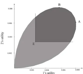
pairs of exchange equilibrium indirect utilities for every possible value of y _∈ Y ∩ (−2,0]×R2

+

[image:9.595.216.384.434.584.2]

.

Figure 1: Exchange equilibrium utilities

As the picture shows, the two owners of the firm disagree on the most preferred production plan. If investor 1 were the only one deciding on the firm’s production plan (i.e., he were the controller of the firm), then he would choose y_A = −2

3,

√

2 3 ,

2 3

= arg maxU1_{(y), which corresponds to point A on}

−23, 2 3,

√

2 3

= arg maxU2(y), i.e., point B. If they both control the firm, their disagreement poses problems for defining an appropriate objective for the firm.

If the firm’s objective were to maximize its market value, the optimal choice would be y∗ = 0. This choice gives firm’s owners an utility of 0 and thus the value maximizing production plan is the worst possible outcome for each

owner.

Although an unanimously approved plan does not exist, we believe that a desirable property of an equilibrium outcome in this environment is that of being, at least, Pareto undominated from the shareholders’ point of view. On these grounds, one must eliminate, as possible equilibrium outcomes, all points that do not lie along the frontier between the points A and B. If, for instance, point E were the equilibrium outcome then shareholders would have an incentive to renegotiate to a better alternative in the shaded area of figure 2, and thus the firm would be vulnerable to a take-over. For this reason we view pointE as an “unstable” and thus undesirable equilibrium outcome.

We are proposing here an objective for the firm which selects (some) pro-duction plans that are efficient from the shareholders’ point of view. Clearly, the maximization of a weighted average of the shareholders’ indirect utilities has this property. However, different utility representations of shareholders’ preferences would generate different objectives for the firm and different opti-mal choices: a highly undesirable feature! We are therefore interested in finding an objective for the firm which is independent of the utility representations of shareholders’ preferences, while still delivering equilibrium outcomes that are stable to shareholders’ renegotiation4_{. This paper proposes a way of}

construct-ing such an objective.

3

The Simplified Model: Equity-Financed

Pro-duction

Consider an economy that lasts for two periods, t= 0,1. There areS possible states of nature at date 1 and only one non-storable consumption good per date and state.

The economy is populated byI consumers/investors, and there is one firm. Firm’s production possibilities are described by the convex and closed subset

Y _{⊆ R− × R}S

+. A typical element of Y is of the form y = (y0, y1, ...yS),

where ₋y0 represents the amount of input put into production (or investment

made) at date 0, and ys is the amount of output produced at date 1 if state s

occurs. Investors are characterized by their preferences over state contingent consumption plans and their endowments of goods and shares in the firm’s profits. Investor i is endowed with the vector ωi _{= (ω}i

0, ωi1, ..., ωiS) ∈ R S+1 ++

of state-contingent consumption goods and δi _∈ [0,1] shares in firm’s profits. His/Her preferences over consumption streams c = (c0, c1, ...cS) ∈ RS++1 are

represented by the continuously differentiable, increasing in every argument and strictly quasi-concave utility function ui _:RS+1

+ →R.

Let C _⊆ I5 be the set of investors who control firm’s decisions; we call them thecontrol group. One could think of C as being, for example, the Board of Directors. Members of the control group can be shareholders as well as non-shareholders of the firm (for example, a non-shareholder employee of the firm can be a member of the control group). Let δC def= P_i∈Cδi be the aggregate share holdings by members of the control group.

The only way of transferring consumption among dates/states is through trade in firm’s shares. They are available for trade at time 0 and pay dividends at time 1. Short sale of firm’s shares is allowed for up to L units, where L _∈

[0,+_∞] is exogenously given. L = +_∞ means that unlimited short sales are allowed.

For now, it is assumed that the firm’s sole decision is to select a feasible production plan y _∈ Y (i.e., it is implicitly assumed that the firm finances its production/investment only by issuing equity). In section 4 we relax this as-sumption and analyze the situation in which the firm takes not only production, but also more complex financial decisions.

Investors choose their share holdings and the amount of goods they want to consume in every date/state such that to maximize their utilities and satisfy their budget constraints at every date and state. It is assumed that the number of investors,I, is large enough, so that their behavior can be approximated by the familiar price taking hypothesis. This means that they act in the belief that their portfolio and consumption decisions do not affect the price of the security available for trade in the assets market. However, those investors that are members of the control group do understand the effect offirm’s production choices on the share price. We assume that, for every production plan that the firm may choose, they are able to anticipate correctly (some of) the corre-sponding equilibrium share price(s). We say that members of the control group haverational price perceptions.

Given some production plan, y, and price of shares, v, consider agent i’s optimization problem as an investor,

      

maxθ,cui(c)

s.t. c0+θv =ω0+δi(v+y0) cs =ωs+θys s= 1, .., S

θ _{≥ −}L, c0, c1, ...cS ≥0,

(1)

and let ci_{(y, v), θ}i

(y, v) be its solution.

An equilibrium price of the stock-exchange economy corresponding to y is

5

any real number, v, that solves: PI_i=1θi(y, v) = 1. Let Qe (y) denote the set of all solutions. Qe is thus a correspondence fromY to_R. Let Yb be the set of production plans for which Qe (y) is non-empty.

To simplify matters, we assume here that the control group’s (rational) price perception is a particular measurable selection, Π,fromQe. [In the next section we will consider the situation in which the control group holds non-degenerate beliefs over possible equilibrium prices.] Therefore Π : Yb _{→ R} is such that Π (y)∈Qe (y),_∀y_∈Yb. Let ci_(y)def_{= c}i_{(y,Π (y)) andθ}i

(y)def= θi(y,Π (y)).

The price perception Π and utilities (ui₎

i_∈C induce members’ preferences

over firm’s production plans as represented by the indirect utilitiesVi

Π:Yb →R,

where Vi

Π(y)

def

= ui_(ci_{), for every i∈C.}

The next definition introduces our notion of C-efficiency, i.e., efficiency from the control group members’ point of view. The basic idea is the following. Suppose that the economy is at a status-quo at which the firm’s production plan is ¯y. If there exists an alternative plan, y, and a system of date-0, after-trade side payments that improve every member’s utility, then the control group has an incentive to move away from the status-quo plan by adopting y and implementing the transfers. We are interested in production plans ¯y that are stable to such arrangements. Those production plans are calledC-efficient.

Definition 3.1 A production plan y _∈ Y is C-efficient (given the price per-ceptionΠ) if there does not exist a vector y,(τi₎

i∈C

consisting of a production plan y _∈Y and date-0 transfers (τi₎

i∈C ∈R

C _satisfying:

i) Pτi _≤0,

ii) ui_(ci_{(y) +τ}i_e

0)≥VΠi (y) for every i∈C, iii) uj_(ci_{(y) +τ}i_e

0)> VΠi(y) for some j ∈C,

where e0 = (1,0, ...,0)∈RS+1.

Note that this concept ofC-efficiency is different from Dr`eze’s original con-cept in that investors are allowed to adjust their shares in response to a proposed change in the production plan of the firm. It also differs from Grossman-Hart’s concept in the type of price perceptions used for defining members’ preferences over production plans.

In the remaining of this section we construct an objective of the firm that generates C-efficient production plans in equilibrium. To do that we measure – in units of date-0 consumption – the change in each investor’s welfare due to a change of the production plan fromy_etoy.

Let εi₍

e

y, y) denote the minimal amount of date-0 consumption good that investor i must be compensated with, in order to accept a change from _ey to y

(i.e., to accept a change from the consumption planci₍

e

y,Π (_ey)) toci_{(y,Π (y))).}

Thusεi₍

e

y, y) satisfies:

Clearly, εi₍

e

y, y) _≥ 0 if and only if investor i weakly prefers production plan y_e

toy, i.e., V_Πi(ey)_≥V_Πi(y).

Since ui _{is quasi-concave, relation (2) implies:}

(ci₀(y) +εi(y, y_e ), ci1(y)₋(ci₀(y_e), ci1(_ey))_∇ui(ci₀(y_e), ci1(_ey))_≥0, (3)

where∇ui _{denotes the gradient ofu}i_{.Using investori’s budget constraints and}

rearranging terms, (3) becomes:

εi(_ey, y)_≥δi(Π (_ey) +y_e0) +θi(ye) M RSi(ye)ye1−Π (ey)

−

−δi(Π (y) +y0) +θi(y) M RSi(ye)y1−Π (y)

,

whereM RSi₍

e

y)def= M RSi_(ci₍

e y)) =

∂1ui_(eci₎

∂0ui_(eci₎, ...,

∂Sui(eci)

∂0ui_(eci₎

is investori’s marginal rate of substitution between consumption at date 1 and consumption at date 0.

Let Wi

e

y(y) def

= δi(Π (y) +y0) +θi(y) (M RSi(ye)y1−Π (y)). If W_eyi(ye) ≥

Wi

e

y(y) then ε i₍

e

y, y)_≥ 0 and thus investor i weakly prefers6 _{production plan ye}

overy.

Definition 3.2 For a given price perception Π and every ey, y∈Yb let

VC

e

y,Π(y)

def

= X

i_∈C

Wi

e

y(y) = δ C

(Π (y) +y0) + X

i_∈C

θi(y) M RSi(y_e)y1₋Π (y),

where δC def= P_i∈Cδi is the initial aggregate share holding of the control group.

VC

e

y,Π(y) is called the C-adjusted value of y at ey.

The C-adjusted value is the firm’s value as perceived by the members of the control group. It is the sum of the market value of the control group’s initial share of the firm, δC(Π (y) +y0), and the value that the control group

attributes, at y,_e to trading in firm’s common stock as a risk-hedging instru-ment,

X

i_∈C

θi(y) M RSi(_ey)y1₋Π (y). (4)

For everyi,M RSi₍

e

y)y1 is an estimate of the investori’s valuation of the secu-rity y1, and thusM RSi(ye)y1−Π (y) is a measure of the surplus, to investori,

from purchasing one unit of the securityy1_{.Therefore, expression (4) represents}

the control group’s aggregate surplus from trading firm’s equity.

6_{Note, however, that}

Wi e

y:Yb →Ris not a utility representation of investori’s preferences

over production plans sinceVi

Π(ye)≥V

i

Π(y) does not necessarily imply W

i e

Accounting for this surplus in the firm’s objective is essential for obtaining

C-efficient production plans at the equilibrium and the significance of the firm’s financial policy (see section 6). Grossman-Hart’s assumption of “competitive price perceptions” implies that investors behaveas if trading in firm’s common stock generates no surplus (or loss) for them. Therefore, term (4) is neglected from the computation of the firm’s objective. As we will show in section 5, this is an entitled omission if the firm is competitive. However, if the firm has some market power, the surplus given by formula (4) is different than zero and should be taken into account.

If C=I, the C-adjusted value is

VI

y,Π(y) =y0+ "

X

i∈I

θi(y)M RSici

# y1.

This is the firm’s market value computed under a system of state prices equal to the average of the shareholders’ marginal rates of substitutions weighted by their final share holdings. This is similar to Dr`eze objective, except that the weights vary withy.Thus, in contrast to Dr`eze and Grossman-Hart objectives7_,

the C-adjusted value is not a linear function of y.

Definition 3.3 An equilibrium of the production economy consistent with the control group’s price perception Π is any vector y,ci, θi

i_∈I, v

∈ Yb _× RS

+×R I

×R+ that satisfies the following conditions:

i. ci_{, θ}i

i_∈I solves (1) given the price v,

ii. v = Π (y),

iii. y_∈arg max_y∈YbV

C y,Π(y),

iv. P_i∈Ici =y+P_i∈Iωi.

Theorem 3.4 In every equilibrium the firm’s production plan is C-efficient.

The proof of this proposition is given in section 4.4 in a more general context.

ForC =I theorem 3.4 is a first welfare theorem type of result. It says that the equilibria of the production economy areminimallyconstrained efficient8_{, in}

the sense that the equilibrium allocations cannot be improved upon by a social

7_{With the notation of this paper, Dr`eze’s objective is}

Dy(y) = y0 +

P

i∈Iθ i

(ye)M RSi₍

e

y)y1_{,while Grossman-Hart’s is}

GHy(y) =y0+P_i∈IδiM RSi(ye)

y1_. 8

planner who can choose the production plan and redistribute consumption at date 0,but has to use the markets to purchase the date-1 consumption for every investor. The formal definition of this efficiency concept follows.

Definition 3.5 An allocation y, ci₀, ci1(y)_i

∈I

is minimally constrained ef-ficient given Π if and only if:

1. P_i∈Ici

0 = P

i∈Iω i

0+y0,

2. there does not exist a Pareto superior allocation y,(ci₀, ci1(y))_i∈I such that P_i∈Ici

0 = P

i∈Iω i

0+y0.

The next corollary is an immediate consequence of theorem 3.4.

Corollary 3.6 If C =I, every equilibrium is minimally constrained efficient.

Note that minimal constrained efficiency is weaker than constrained Pareto optimality. A planner could, potentially, improve upon a minimally constrained efficient allocation by redistributing shares (or, equivalently, using before trade date-0 transfers). Therefore, even when C = I, equilibria in which the firm maximizes itsC-adjusted value are not, in general, constrained Pareto optimal.

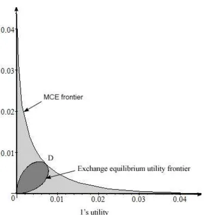
Example 2 To illustrate the results of this section, consider again the example of section 2. If C = {1} (or C = {2}), the unique C-efficient out-come is point A (respectively B). This corresponds to the production plan

y_A = −2

3, √ 2 3 , 2 3

(respectively y_B = −2 3, 2 3, √ 2 3

). The firm’s C-adjusted value (at yA) is V{

1}

y_A (y) = 2 (1 +y0) + 1₃

√

2y1 + 2y2

, which is maximized at

−2 3, √ 2 3 , 2 3

. Thus y_A is the unique equilibrium production plan ifC ={1}. Suppose now thatC =_{1,2_}.An allocation y, c1₀,1₂y₁,1₂y₂, c2₀,₂1y₁,1₂y₂

is minimally constrained efficient (MCE in the sequel) if and only if (y, c1 0, c20)

solves max   λu 1

c1₀,1

2y1, 1 2y2

+ (1₋λ)u2

c2₀,1

2y1, 1 2y2

| c1₀+c2₀ = 2 +y0 c1₀, c2_{0 ≥}0

 



for some λ _∈ [0,1]. The parametric equation of the MCE frontier (in utility coordinates) is given by

8

3 −6 (y1) 23y1

2

1 6 −

(y1)2

4

, 6 (y1)2− 4₃ 3 (y1)2

4

√2 3−(y1)

2

2

.

[image:16.595.203.403.74.284.2]

Figure 2: Minimally constrained efficient frontier

and therefore the only candidate for an equilibrium production plan. Straight-forward computations show that yD =

−2 3,

√

3 3 ,

√

3 3

maximizes the adjusted valueVy{D1,2} and thus it is an equilibrium production vector.

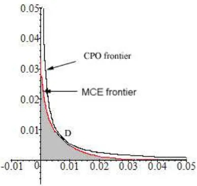
Although in this exampleC =I,the minimallyC-efficient production plans are not necessarily constrained Pareto optimal. Figure 3 illustrates that. How-ever, since the two frontiers intersect in pointD the equilibrium corresponding to C = _{1,2_} is constrained Pareto optimal. In section 5 we will show that this is a more general result, that applies to economies in which the firm has no market power in the financial markets. Indeed, in this example, the firm does not influence the markets by making its equity contract available for trade, because in every exchange equilibrium, consumers choose not to trade firm’s shares.

4

The General Model

[image:17.595.200.394.96.279.2]

Figure 3: CPO versus MCE

4.1

The Economy

The market participants have the same characteristics as described in section 3. The market structure is different in that there are J < S exogenously given securities available for trade at date 0. Security Aj _{pays a}

js units of the

state-contingent consumption good if state s occurs. The matrix A def= (ajs)j=1..J s=1..S ∈

MS×J(R) is called the payoff matrix.

The firm can finance its production plan by borrowing in the existing se-curity markets and issuing new shares and/or securities9_{. We assume that the}

firm cannot issue more thanM new shares and is allowed to design exactly N

firm-specific securities10_{. N is taken to be large enough}11 _{so that the firm has}

the capacity to complete the markets (if that is optimal for its control group). The payoffs of the securities that the firm may issue to finance a produc-tion plan y are constrained to lie in some exogenously given set K(y) ⊆ RS_.

The set _K(y) encompasses the restrictions that firm faces when issuing new securities. For example, the firm may be constrained to issue only securi-ties with positive payoff in every state, in which case K(y) ⊆ RS

+.

Alterna-tively, _K(y) _{⊆ {}(f(y1), ..., f(yS))|f :R→R} means that the firm can issue

only derivatives on its equity (such as options on equity). It is assumed that

0S ∈ K(y) andy1 _{∈ K(y),so that the firm can always choose the trivial}

finan-9 _{Examples of such firm-issued securities are convertibles, warrants, floating-rate debt,} zero-coupons, primes and scores, etc.

10_{This assumption is made to simplify the technicalities of the model. However, since the} firm is allowed to issue securities with zero payoff in all states, the constraint merely imposes an upper bound on the number of new securities the firm may issue.

11

cial structure _{0S, ...,0S,y1_},where0S is the zero vector in _RS_{. Let alsoM be}

the exogenously given upper bound on new equity issues.

For every j _{∈ {}1, ..., J +N + 1} investors are allowed to sell short up to

Lj ∈[0,+∞] units of the security j.The same constraints are faced by the firm

for its trades in the exogenously given securities. Let L def= (L1, ..., LN+J+1)

denote the vector of portfolio bounds.

The firm has to decide on: (a). a production plan y _∈ Y, (b). a stream of dividends D _{∈ R}S _{to be paid to its shareholders at date 1, (c). a matrix}

of payoffs X _{∈ M}S_×N(R) for the N securities to be issued, (d). a portfolio12

bf _∈RJ of asset holdings and (e).a number θf _∈Rof new shares to issue.13 _A

vectorP = y, D, X, bf_{, θ}f

∈Y_×RS_×M

S_×N(R)×RJ+1is called a

production-financial plan/policy.

Definition 4.1 A production-financial plan y, D, X, bf, θf is called feasible if:

i. y_∈Y

ii. D, Xn ∈ K(y), for every n ∈ {1, ..., N}, where Xn denotes the n-th column of X,

iii. θf _∈[₋1, M] and bf_{j ≥ −}Lj for every j ∈ {1, ..., J},

iv. y1 _{= 1 +θ}f_D

+Abf _{+X1N, where 1N = (1, ...,1)}t

∈RN_.

The set of all feasible plans is denoted by _F.

If the firm chooses production-financial plan _P = y, D, X, bf_{, θ}f _and

(q, p, v) _{∈ R}J _{× R}N _{×R are the market prices of the already existing}

secu-rities, the firm-issued securities and the dividend stream, then the firm’s profit at date 0 is

D0

def

= y0+qbf +p1N +θfv.

This is distributed to firm’s shareholders according to their initial shares14_.

Therefore, if the firm chooses policy _P = y, D, X, bf_{, θ}f

, having an initial endowment of δ shares is equivalent, in terms of wealth generated, to receiving

δy0 units of the date-0 consumption good and being endowed with a portfolio δbf_{, δ1N, δθ}f

of the J+N + 1 traded securities.

Hence, every feasible production-financial plan P, generates the following (artificial) stock-exchange economy:

12 _{To simplify notation we are assuming that portfolio holdings are column vectors.} 13_{A negative value of}

θf indicates that the firm repurchases₋θf of its outstanding shares. A positive value indicates that firm is issuingθf additional shares.

14 _{The situation described in section 3 corresponds to the case in which}

D0 = y0, D1 =

y1

∈RS+1

, bf _{= 0}

∈RJ_{, θ}f

EP = ((ui, ωi0+δ

i

y0, ω1i

, δibf, δi1N, δiθf)i, A, X, D).

In EP every investor i takes the asset prices as given and chooses his/her

consumption and portfolio by solving:

      

maxci_,bi_,ri_,θiui(ci)

s.t. ci

0+qbi+pri+vθi =ωi0+δi y0+qbf +p1N +vθf

ci1 _=ωi1_+Abi_+Xri_+Dθi

ci _{≥0, b}i_{, r}i_{, θ}i

≥ −L.

(5)

Definition 4.2 An equilibrium of the stock-exchange economy _EP consists of prices, (q, p, v), consumption allocations, ci

i=1...I, and securities holdings,

bi, ri, θi

i=1...I, such that the following conditions are satisfied:

1. ci_{, b}i_{, r}i_{, θ}i

i=1...I solves (5) given the prices (q, p, v),

2. all markets clear, i.e.,

I

X

i=1

bi = bf,

I

X

i=1

ri = 1,

I

X

i=1

θi = 1 +θf

I

X

i=1 ci =

I

X

i=1

ωi+y.

4.2

Control Group’s Price Beliefs

The control group’s beliefs are positive probability measures over the space of asset prices. The beliefs are rational in the sense that they assign zero proba-bility to all prices that are not among the equilibrium ones. Their construction is shown in the sequel.

For every _P = y, D, X, bf, θf _{∈ F} let Qe (_P) _{⊆ R}J+N+1 _{be the set of}

equilibrium asset prices of EP. Define Yb

def

= ny _∈Y _|y0 ≥ −min

ωi

0 δi +ε

o

and

b

F def= nP = y, D, X, bf_{, θ}f

∈ F |y_∈Ybo, where ε > 0 is arbitrarily small. Then Qe (P)6=∅ for every P ∈Fb (see the appendix for a proof). We restrict15

the firm’s choices to the feasible production-financial plans in _Fb.

LetMbe the space of all measurable selections fromQe. We endowMwith the product topology and consider the associated Borelσ-algebra, _B(_M).

Definition 4.3 Any probability measure, µ, over (M,_B(M)) is called a ra-tional belief for the control group.

4.3

Firm’s Objective and the Equilibrium Concept

The firm’s objective is to maximize theexpected C-adjusted value, given control group’s beliefs over the set of equilibrium prices. As in the model of section 3, theC-adjusted value will be defined as the sum of the fraction of firm’s market value received by the members of the control group as initial shareholders and a measure of the members’ surplus from their transactions in the stock markets. Since investors can trade in many securities, the surplus acquired from their trade inevery marketed security must be taken into account.

We introduce first some notation.

Let µ be control group’s price belief, Π = (q, p, v) ∈ supp(µ) an arbitrary price functional in the support ofµand_{P ∈F}ban arbitrary financial-production plan in the firm’s action set. Then:

1. Π_P(l) is the price of security l _∈n(Aj₎

j=1,...,J, D,(X n₎

n=1,...,N

o

given by

the pricing functional Π. For example, if l =D, then Π_P(l)def= v(_P),

2. Z_Pi (l) is consumeri’s optimal holding of security l at prices Π (_P),

3. Z_PC(l)def= P_i∈CZyi (l),

4. ci_{(P) is investor i’s optimal consumption in the economy E}

P, at prices

Π (_P).

Definition 4.4 For P, P ∈ Fb and a given Π ∈supp(µ) we define the C -adjusted value of _P at _P as:

VC

P (P)

def

= δC(Π_P(D) +D0) +W_P(P), (6)

where

D0 = y0+q(P)bf +p(P)1N +v(P)θf and

WP(P) =

X

l_∈(Aj)j,(Xn)n,D

Wl

P(P),

Wl

P(P) =

X

i∈C

Z_Pi (l)M RSi ci _Pl₋Z_PC(l) Π_P(l).

Similarly to our discussion in section 3, we interpret the expression

Z_Pi (l) M RSi cil₋Π_P(l)

as investori’s surplus from trading securityl.ThusWl

P(P) measures the control

group’s surplus from trading l and _WP(_P) is the surplus from all its transac-tions in the stock markets.

portfolios may not be unique. Investors who trade in at least one redundant security are, in fact, indifferent among a continuum of portfolios. The C -adjusted value is well-defined if and only if it is invariant to the choice of optimal portfolios. Next proposition shows that this is indeed the case.

Proposition 4.5 TheC-adjusted value is well-defined.

Proof. Let Π _∈ supp(µ), (_P,_P)_{∈ F ×}b _Fb and (Zi

P(l))l∈(Aj)j,(Xn)n,D

i∈C

a vector of optimal portfolios for the members of the control group. Using every investor i’s budget constraint (i_∈C) and rearranging terms in (4.4) we obtain:

VC

P (P) =

X

i_∈C

ci₀(_P)₋ωi₀+X

i_∈C

M RSi ci1 _P ci1(_P)₋ωi1. (7)

Since ui _{is strictly quasi-concave, the optimal consumption stream c}i_(P)

is unique and thus the value of _VC

P (P) is independent of the choice of the

members’ optimal portfolios.

The firm’s objective is to maximize its expectedC-adjusted value, given its beliefs. This means, max_PEµ_(VC

P (P)) =

R

MV

C

P (P)dµ(Π). Note that the

in-tegralR_MVC

P (P)dµ(Π) is well-defined because, given the product topology on

M, the mapping Π _7−→Π (_P) from _Mto _RJ+N+1 _{is continuous (and thus}

in-tegrable) for every_P. Moreover, consumers’ demands for goods are continuous functions of prices.

Letµ denote the control group’s rational beliefs over the set of equilibrium asset prices.

Definition 4.6 An equilibrium of the production economy consists of: (1). some rational belief, µ, (2). a production-financial plan _{P ∈ F}b for the firm, (3). a consumption-portfolio allocation for the investors, ci_{, b}i_{, r}i_{, θ}i

i=1...I,

and (4). a system of prices, (q, p, v), such that:

i. consumption-portfolio allocations are optimal within each investor’s bud-get constraint, i.e., ci_{, b}i_{, r}i_{, θ}i

i=1...I solves (5) given (q, p, v),

ii. beliefs are consistent with the equilibrium prices, i.e., there exists Π _∈

supp(µ) such that (q, p, v) = Π _P,

iii. the firm maximizes its expected C-adjusted value at P, given the beliefs

µ, i.e., _{P ∈}arg max_PR_MVC

P (P)dµ(Π),

4.4

C

-efficient Policies

We say that a production-financial plan isnotC-efficient if forevery price in the support of the control group’s beliefs, there exists another production-financial plan and a system of date-0 transfers that lead to an improvement in everyone member’s utility. The formal definition follows.

Definition 4.7 Let µ be the control group’s beliefs over _M. A production-financial planP is notC-efficient (givenµ)if there exists a production-financial plan _P and a system of date 0 transfers (τi₎

i∈C such that,

P

τi _{≤ 0 and, for}

every Π_∈ supp(µ), a) ui_(ci_{(P) +τ}i_e

0)≥ui ci P

for every i_∈C,

b) uj_(ci_{(P) +τ}i_e

0)> uj ci P

for some j _∈C.

Theorem 4.8 In every equilibrium of the production economy the firm’s production-financial plan is C-efficient.

Proof. Let _P be an equilibrium production-financial plan corresponding to belief µ. If it is not C-efficient then there exists an alternative plan,P, and a system of transfers at time 0,(τi₎

i∈C, such that

P

i∈Cτ

i _{≤ 0 and, for every}

Π ∈ supp(µ), ui_(ci_{(P) +τ}i_e

0) ≥ ui ci P

∀i _∈ C, with at least one strict inequality for some j _∈C.

Strict quasi-concavity of ui implies that:

ci₀(_P) +τi₋ci_{0 P}+M RSi ci _P ci1(_P)₋ci1 _P≥0,

for every i_∈C, with strict inequality for some j _∈C.

Adding up over i_∈C and using P_i∈Cτi _{≤0 yields}

X

i_∈C

ci₀(_P)₋ci_{0 P}+X

i_∈C

M RSi ci _P ci1(_P)₋ci1 _P>0,

or, equivalently,

X

i∈C

ci₀(P)−ωi₀+X

i∈C

M RSi ci _P ci1(P)−ci1 _P>X

i∈C

ci_{0 P−}ωi₀.

(8) Using (6), inequality (8) becomes VC

P (P) > V

C

P P

. Integrating this last in-equality over Π _∈ supp(µ) we obtain Eµ _VC

P (P)

> Eµ _VC

P P

which is a contradiction with the equilibrium condition (ii).

5

Shareholders Unanimity and Firm’s Market

Power

In this section we restrict attention to firms whose production choices have no impact on the market prices. We call such firm competitive in the goods markets.

If, in addition, the spanning condition holds (i.e.,_K(y)_⊆span(A) for every

y _∈Y) any security that the firm may issue is replicable by a portfolio of the exogenously given assets, and thus a change in the firm’s financial policy has no influence on the market equilibrium either. Thus the firm is competitive in both, the goods and the financial markets. In this case, its C-adjusted value coincides with the (unambiguously defined) market value and is independent of the choice of the financial policy. Modigliani-Miller theorem holds and the firm’s shareholders unanimously agree on the value-maximizing production plan.

If spanning does not hold (i.e.,K(y)"span(A) for at least somey_∈Y), a firm that is competitive in the goods market may still influence the equilibrium prices through its issuing of new securities. As shown by Diamond in [5], shareholders’ unanimity can still be obtained in this case if the firm’s production set projects on _RS _{along an 1-dimensional subspace.}

This section identifies more general conditions under which unanimity of the firm’s shareholders on the most preferred production-financial plan obtains. We show that, when concerned with the shareholders’ unanimity for all profiles of preferences, spanning and the Diamond-type technology are necessary and suf-ficient conditions. For particular subclasses of preferences (i.e., linear risk tol-erant and mean-variance), less restrictive conditions are sufficient to guarantee the shareholders’ unanimity.

Definition 5.1 A firm is said to be competitive in the goods markets if and only if, for any feasible plans_P and_P′ _{for which span(A, X, D) =span(A, X}′_{, D}′_),

it is true that Π_P(l) = Π_P′(l) for every l ∈span(A, X, D).

LetX _⊆R−×R+ be an arbitrary set with 0∈X and ϑ∈RS+ an arbitrary

vector. We say that a firm has a Diamond-type technology if its production set is of the form Y def= _{(y0, ϑk)|(y0, k)∈X}, and K(y) = {0, ϑk} for any y= (y0, ϑk)∈Y. Therefore, a firm with Diamond-type technology is restricted

to finance its production by issuing only equity, and may expand the asset span along a single direction.

Proposition 5.2 For a firm that is competitive in the goods markets and has a Diamond-type technology, the maximization of the (expected) C-adjusted value coincides with the maximization of the (expected) market value, which is unan-imously supported by all shareholders.

Proof. Since the firm is restricted to issuing equity only, its C-adjusted value is:

VC

y (y) =δ

C _{Π y}1_+y 0

+X

i_∈C

Since y1 and y1 are colinear and the firm is competitive in the goods markets,

M RSi(y)y1₋Π (y1) = 0 and thus _VC

y (y) =δ C

(Π (y1) +y0).

As proved above, shareholders’ unanimity is obtained if the firm’s technology satisfies the spanning property or is of the Diamond-type. These restrictions on the firm’s technology are also necessary for obtaining the shareholders’ una-nimity within the entire class of rational preference profiles. In other words, if the firm’s technology does not satisfy the spanning property and is not of Diamond-type then, by appropriately choosing the shareholders’ preferences, one can construct economies in which shareholders disagree on their most pre-ferred production-financial plan.

Therefore, obtaining shareholders’ unanimity for all arbitrary profiles of their preferences imposes strong restrictions on the firm’s technology. By con-trast, within the class of market economies in which consumers have either mean-variance or linear risk tolerance utilities, shareholders’ unanimity is ob-tained for any technology. In such economies, the firm’s objective renders its financial policy trivial and the maximization of theC-adjusted value coincides with Grossman and Hart’ value maximization.

Definition 5.3 Let y _∈Yb and(ci₎

i∈I be a feasible consumption allocation for

the exchange economy corresponding toy.(i.e.,P_ici _=y+P

iωi).Then (ci)i_∈I

is called distribution-efficient if it is Pareto optimal in the exchange economy corresponding to y.

Proposition 5.4 (LRT utilities) Suppose that the exogenously given asset market contains the risk-free bond, as well as every investor’s initial endow-ment of goods. If investors’ preferences can be represented by expected utilities with linear risk tolerance and positive identical slopes, then the firm’s financial policy is irrelevant and the equilibrium allocation is distribution-efficient. If, moreover, C =I, the equilibrium production plan,y satisfies:

y_∈arg maxy0+M RS(y)y1 ,

where M RS(y) denotes investors’ common intertemporal marginal rate of sub-stitution.

Proof. If investors’ utilities have linear risk tolerance with the same slope, then every distribution-efficient allocation can be achieved by holding a port-folio composed of the risk-free and the market security (i.e., the aggregate endowment). Since for every financial policy that finances a production plan

y the asset span contains both the risk-free bond and the market security, all distribution-efficient allocations corresponding toyare in the asset span. More-over, since every feasible allocation (for the exchange economy corresponding to

it follows that every exchange equilibrium in the associated stock-market econ-omy has the two-fund spanning property and thus all financial policies generate the same equilibrium consumption stream as the equity-financed plan. There-fore, the financial policy is irrelevant in this case (consequence of proposition 4.5) and the equilibrium allocation is distribution-efficient.

Since the equilibrium is distribution-efficient, investors’ intertemporal marginal rates of substitutions are equal, and thusM RSi_{(y) =M RS}j_(y)def_{= M RS(y) for}

everyi, j _∈I.IfC =I thenθC(y) = 1 and thusy_∈arg max_{y0+M RS(y)y1}.

Suppose now that investors’ utilities ui are quasi-concave and satisfy:

ui ci=hi ci₀, E ci1, var ci1, _∀i_∈I

withhi _{differentiable, increasing in the first two variables and decreasing in the}

third. Suppose, as in the previous example thatC =I and the risk-free bond, as well as investors’ initial endowments of goods are in the asset span.

Proposition 5.5 (CAPM Equilibrium) Under the above stated assump-tions, the equilibrium allocations are Pareto optimal and firm’s equilibrium pro-duction plan satisfies:

y_∈arg maxy0+M RS(y)y1 . (9)

Proof. Given the particular preferences, every equilibrium production plan

y generates distribution-efficient consumption allocations (see Magill-Quinzii [18], pp. 181-183 for a proof). Then, as before, investors’ marginal rates of substitution are equalized at the equilibrium and firms’ objective becomes the one in formula (9).

5.1

Competitiveness in Financial Markets

As emphasized before, if the spanning property holds, a firm’s financial policy alone has no influence on the market equilibrium. We identify here more general conditions that guarantee firm’s competitiveness in the financial markets and analyze their equilibrium implications. We show that if a firm is competitive in the financial markets, then its C-adjusted value is unaffected by the financial policy and thus it is irrelevant how the firm finances its investment. If the firm is competitive in both, the financial and the goods markets, itsC-adjusted value coincides with the Grossman-Hart objective. If, in addition, there is no production-specific risk, i.e., if Y ⊆ span(A) (one instance in which this happens is if markets are complete, i.e., span(A) = RS_{), then the C-adjusted}

We assume, throughout this section that unlimited short sales are allowed. For everyy_∈Y consider the artificial stock-exchange economy_E0

y in which

the market structure is given by the payoff matrixA,investors’s preferences are the same as before, their endowments of goods areωi_+δi

yand their endowments of securities are 0. _Ey0 is therefore an imaginary stock-exchange economy in

which firm has committed to producing y but its stock is not traded in the market. For every l_∈RS_{, let E}l

y be the economy with the same characteristics

as_E0

y, except that its market structure is given by (A, l)∈ MS×(J+1).

LetYb be the set of production plans for whichE0

y has a stock-exchange

equi-librium and assume that the equiequi-librium is unique16_{. Let that be (c}i_{(y), b}i_{(y), q(y))} i∈I.

Define

Dy def

= l _∈RS _|M RSi ci(y)l =M RSj cj(y)l, _∀i₆=j _∈I .

The set Dy is called the extended asset span corresponding to y. Clearly,

span(A)_{⊆ D}y,but the inclusion may be strict. Ifspan(A)$Dy and the

equi-librium consumption allocation (ci(y))_i∈I is interior, then any security whose payoff lies in Dy\span(A) has the property that, if introduced into the

mar-ket, it does not change the equilibrium prices or allocations. The following proposition states this property formally.

Proposition 5.6 Let l _{∈ D}y \span(A) and p(y) = M RSi(ci(y))l, i ∈I. If

(ci_(y))

i_∈I is interior, then consumption allocation(ci(y))i_∈I, portfolio holdings

(bi(y),0)_i∈I and prices (q(y), p(y)) form an equilibrium of the economy _El y. Proof. Sinceci(y)_≫0_∀i_∈I andp(y) = M RSi(ci(y))l =M RSj(c(y)j_)l,

∀i ₆= j _∈ I, the first order conditions for the consumption choice in El

y, given

(q(y), p(y)),are satisfied at (ci_(y))

i∈I.Quasi-concavity of investors’ utility

func-tions imply that the first order condifunc-tions are sufficient and thus

ci(y), bi(y),0_i

∈I,(q(y), p(y))

is an equilibrium inEl y.

Definition 5.7 We say that the firm is competitive (or has no market power) in the financial markets if _K(y)_{⊆ D}y for every y∈Yb.

If the firm is competitive in the financial markets, any security it may issue has no effect on the equilibrium prices of the other traded securities or on the equilibrium consumption allocations. Therefore investors are indifferent between having the markets for the firm-specific securities open or closed. Being competitive in the financial markets doesnot mean that the firm’s decisions do not influence the markets. It means only that itsfinancial policy has no impact on the markets. However, changes in the production plan can still affect prices.

If the firm is competitive in the financial markets then, for every feasible production-financial plan _P = y, X, D, θf, bf, there exists an exchange equi-librium of EP in which investor i’s holdings of firm’s securities are: ZPi (D) =

δi 1 +θf and Zi

P(l) = δ

i

,_∀l _∈ nX1, ...XNo_{. Since holding a share δ}i

of the firm is equivalent to holding that fraction of the firm’s portfolio, the last con-dition actually says that, if the firm is competitive, investors’ net trades in the securities issued by the firm are zero.

Competitiveness in the financial markets implies that theC-adjusted value is invariant to changes in the financial policies. This is an immediate consequence of formula (7) and proposition 4.5. The C-adjusted value of a firm that is competitive in the financial markets is:

VC

P (P) =δ

C

y0+ X

i∈C

δiM RSi ci(y)y1+bC(y) (q(y)−q(y)).

Definition 5.8 The firm is called competitive in all markets (or simply, com-petitive) if it is competitive in both, goods and financial markets17_.

The following proposition shows that theC-adjusted value can be seen as a generalization of Grossman-Hart’s objective, since it coincides with that if the firm is competitive.

Proposition 5.9 If the firm is competitive, itsC-adjusted value coincides with the Grossman-Hart objective.

If, in addition, Yb1 _⊆span(A), _∀y_∈Yb then the C-adjusted value coincides with firm’s market value. Production plans that maximize firm’s market value are every shareholder’s most preferred plans.

Proof. Letµbe the control group’s price beliefs and Π ∈supp(µ) arbitrary. As proved above, competitiveness in the financial markets implies

V_PC(_P) =δCy0+ X

i∈C

δiM RSi ci(y)y1+bC(y) (q(y)₋q(y)),

while competitiveness in the goods market implies q(y)₋q(y) = 0 and thus

VC

P (P) =δ

C_y

0+ X

i_∈C

δiM RSi ci(y)y1.

If span(K(y)) ⊇ Yb1_{, then, in particular, M RS}i _ci_y1 _{= M RS}j _cj_y1

for every i, j _∈ I and all y _∈ Yb. Therefore, investors unanimously support the maximization of the C-adjusted value, which becomes: VC

P (P) = y0 +

M RSi _ci_y1 _=y

0+M RSj cj

y1_{, ∀i, j ∈I.}

The firm in example 1 of section 2 is competitive in financial markets and

C =I. Therefore, for that example, theC-adjusted value and Grossman-Hart objective coincide.

It should be emphasized, that firm’s competitiveness does not imply that Grossman-Hart competitive price perceptions are correct everywhere. They only generate some preferences for the control group’s members whose peaks coincide with their actual most preferred production plans.

Whenever the firm is not competitive, following Grossman-Hart or Dr`eze objective can generate less social welfare for the members of the control group than by maximizing the C-adjusted value.

6

Existence and Pareto Optimality of

Equi-libria

Theorem 6.1 If L_≪ +∞, the mapping y _{7→ K}(y) is upper hemi-continuous and compact-valued and investors’ utilities are strictly increasing in every com-ponent, then an equilibrium in which the firm maximizes the expectedC-adjusted value exists.

The proof of the theorem is delegated to the appendix18_.

An important characteristic of the equilibrium in which firm maximizes its

C-adjusted value is that the financial policy is no longer irrelevant (as it was in Dr`eze’s and Grossman & Hart’s models). Two financial plans that finance the same production plan but generate different asset spans may give different utilities to the members of the control group and thus may be ranked differently. Hence, Modigliani-Miller theorem does not necessarily hold.

Since members of the control group decide the optimal production-financial plan based on their attitudes toward risk and their needs for risk hedging op-portunities, a natural question arises: Is the optimal plan the one that creates a complete asset structure? The answer is in general negative, as shown by the following example. Thus, we should expect an incomplete asset structure to arise at the equilibrium. Given the endogenous market incompleteness, it is not surprising to see that equilibria are, in general, Pareto suboptimal. However, particular types of preferences for the investors do generate Pareto optimal allocations at the equilibrium and thus effectively complete markets (in the terminology of Elul [12]).

Example 3

Consider a two-date economy with three states of nature at date t = 1.

There are two investors and one firm. Firm’s production set consists of only one

plan: Y = _{(₋1,0,₋1,1)_}. This firm can be interpreted as being a financial intermediary that owns the security (0,₋1,1) and incurs a cost of 1 unit of date-0 consumption for trading it in the market. Investors’ characteristics are:

u1(c) = c0+ logc1+ 2 logc2, ω1 = (2,1,2,4), δ1 = 1 u2(c) =c0+ logc3, ω2 = (1,5,0,0), δ2 = 0.

There are no exogenously given assets that can be traded in the market. Suppose first that the firm chooses to finance its plan by issuing only equity. Denote this financial plan by P0. Given P0,the first investor solves

      

max_{c0+ logc1+ 2 logc2}

s.t. c0+θv= 2 +v−1

c1 = 1, c2 = 2−θ, c3 = 4 +θ ci ≥0, i= 0, ..,3

and thus choosesθ1 =−4.

The second investor solves

      

max{c0+ logc3}

s.t. c0+θv = 1

c1 = 5, c2 = 5−θ, c3 =θ ci ≥0, i= 0, ..,3

and chooses θ2 = 1_v for 0< v_≤ 1₅.

The stock market equilibrium dictates then v = 1

5 and thus c 1

0 = 2, c11 = 1, c1₂ = 6, c1₃ = 0, which gives investor 1 an utility Uim1 = 2 + 2 log 6. The firm’s

market value is −1 + 1₅ = −4

5. Using formula (7) to compute the C-adjusted

value we obtain

V_P{10}(P0) = 2−2 +

1,1

3,0

    1 6 0  ₋   1 2 4   

= 4

3.

Assume now that the firm chooses a financial plan that completes the markets. Denote that financial plan by Pc. GivenPc, investors solve

  

max_{c0+ logc1+ 2 logc2}

s.t. c0+p1c1 +p2c2+p3c3 = 2 +p1+ 2p2+ 4p3+ (−1−p2 +p3) ci ≥0, i= 0, ..,3

and

 



max{c0+ logc3}

In equilibrium, p1 = ₄₅6, p2 = 12₄₅, p3 = 1₅ and c10 = 0, c11 = 6, c12 = 6, c13 = 0

which gives investor 1 a utility U1

cm = 3 log 6 < 2 + 2 log 6 = Uim1 . Hence, the

owner of the firm does not want its firm to issue enough securities to complete the markets.

If Pc is chosen, the market value of the firm is −1− ₄₅12 + 1₅ = −16₁₅; the

C-adjusted value of _Pc at P0 is:

V_P{10}(Pc) = 0−2 +

1,1

3,0



   66

0



₋

  12

0

 



= 4

3−7< 4 3.

The example is robust in the sense that the results still hold if we slightly perturb the endowments.

7

Appendix

Proof of theorem 6.1

The proof is based on the observation that, for a given rational belief of the control group, µ, there is a bijection between the set of equilibria of the production economy which are consistent with µand the set of Nash equilibria of a two-player imitation game that will be constructed here.

We start by proving some preparatory lemmas.

Lemma 7.1 The economy _EP has an equilibrium for every _{P ∈F}b.

Proof. Notice first that the economy EP is equivalent to a standard

stock-exchange economy, E0

P, in which

1. consumers’ endowments of goods are ωi_+δi_y i∈I,

2. asset structure is given by (A, X, D),

3. there is no initial endowment of assets,

4. consumers face “personalized” short-sale bounds, Li,P _{∈ R}J+N+1_{, given}

by:

(a) Lj +δibf for every exogenously given security j,

(b) Ln+δi for every firm-issued securityn,

(c) Ld+δi 1 +θf