Simulation of particle motion in a closed conduit validated against experimental data

(1)

Simulation of particle motion in a closed conduit validated against

experimental data

Jindˇrich Dolansk´y1,a

Institute of Hydrodynamics, ASCR, Pod Paˇtankou 5, Prague, Czech Republic

Abstract. Motion of a number of spherical particles in a closed conduit is examined by means of both simula-tion and experiment. The bed of the conduit is covered by stasimula-tionary spherical particles of the size of the moving particles. The flow is driven by experimentally measured velocity profiles which are inputs of the simulation. Altering input velocity profiles generates various trajectory patterns. The lattice Boltzmann method (LBM) based simulation is developed to study mutual interactions of the flow and the particles. The simulation enables to model both the particle motion and the fluid flow. The entropic LBM is employed to deal with the flow characterized by the high Reynolds number. The entropic modification of the LBM along with the enhanced refinement of the lattice grid yield an increase in demands on computational resources. Due to the inherently parallel nature of the LBM it can be handled by employing the Parallel Computing Toolbox (MATLAB) and other transformations enabling usage of the CUDA GPU computing technology. The trajectories of the particles determined within the LBM simulation are validated against data gained from the experiments. The compatibility of the simula-tion results with the outputs of experimental measurements is evaluated. The accuracy of the applied approach is assessed and stability and efficiency of the simulation is also considered.

1 Introduction

Motion of multiple particles in the turbulent flow represents an important application of fluid dynamics. The detailed and accurate description of particle motion in the flow be-longs to difficult problems with many inputs. The motion is determined by the mutual particle-particle, particle-wall and particle-flow interactions and depends on the flow pa-rameters as velocity, solids concentration, density, shape, and size distribution of the conveyed solid objects, the di-ameter and roughness of the pipe. Understanding of under-lying particle-fluid dynamics is important for the safe and economical design of the transport technology.

Transport of spherical particles in a closed conduit with a rough bed is considered as an example of such a process. The particles are conveyed by the water flow defined by the specific velocity profiles. The particles perform both trans-lational and rotational motions, influence the flow around them and undergo collisions with themselves and with the boundaries of the conduit. The bed of the conduit is covered by stationary spherical particles of the size of the moving particles.

The considered system was examined experimentally on a pipe loop with a test section where several trajectories of individual particles were observed. The particles moved mostly in a layer close to the pipe invert, however with in-creasing velocity more particles moved in saltation mode, some of them even freely suspended in the central or upper portion, e.g. [1]

The mathematical model of the system consists of equa-tions for the ﬂuid ﬂow (e.g., Navier-Stokes), equaequa-tions of motion for particles (Newton equations) and equations for velocities before and after (both bed and

particle-a _e-mail:_{[email protected]}

particle) collisions which can be derived from relations for impulse forces.

To solve the flow equations the lattice Boltzmann method (LBM) is used. The LBM is a two decade old numerical ap-proach originating from the lattice gas automata methods (LGCA) used for simulations of complex fluid flows, e.g., [2–4]. The LBM represents a second order and efficient computational scheme – due to its inherent locality and explicitness which enable straightforward parallelization. Moreover, it was shown that the incompressible Navier-Stokes equations can be derived from the lattice Boltzmann equations through the Chapman-Enskog procedure in the limit of long wavelengths as compared to the lattice scale, e.g., [5].

The LBM based simulation is developed to study mu-tual interactions of the flow and the particles. Except it is employed as a flow solver the LBM also enable to com-pute hydrodynamic forces of the fluid acting on the macro-scopic particles. The hydrodynamic forces enter the New-ton equations which are every time step coupled to the lat-tice Boltzmann equations to determine motion of the parti-cles in the flow. Thus the LBM provides a unique compu-tational frame for solving the particle-fluid systems, e.g., [6].

However, the basic LBM is subject to instabilities for the processes described by the high Reynolds numbers. As the considered system is characterized by the Reynolds num-ber up to 105 _{the entropic extension of the LBM is}

em-ployed. The entropic modiﬁcation of the LBM and the en-hanced reﬁnement of the lattice grid yield an increase in demands on computational resources. It is handled by em-ploying the Parallel Computing Toolbox (MATLAB) and other transformations enabling usage of the CUDA GPU computing technology.

!

(2)

4

5

9

7

8

2

1

3

10

11

6

Fig. 1.Layout of the experimental pipeline loop (1-slurry tank, 2-pumps, 3-control valve, 4-ﬂow meters, 5-heat exchanger, 6-transparent section, 7-measurement section, 8-pressure transducer, 9-sedimentation vessels, 10-ﬂow divider, 11-density and discharge measurement).

The trajectories of the particles computed by the LBM simulation are validated against data gained from the ex-periments. The measured velocity profiles serve as inputs of the simulation and correspond to a number of flow rates. The different experimental velocity profiles generate vari-ous particle trajectory patterns.

The compatibility of the simulation results with the out-puts of experimental measurements is evaluated. The accu-racy of the applied approach is assessed and stability and eﬃciency of the simulation is also considered.

This paper proceeds as follows. In the next section, Sect. 2, the experimental tools and material is described. The mathematical model of the process is introduced in Sect. 3. In the following section, Sect. 4, the LBM ap-proach is brieﬂy summarized. The developed simulation is analyzed in Sect. 5. In Sect. 6 the results of the simulation and experiments are presented and discussed. Finally, the conclusions are inferred in Sect. 7.

2 Measurements

The considered system were measured on an experimental pipe loop with a test section of smooth stainless steel pipes with an inner diameter 36 mm, cf. ﬁgure 1. A two meter long transparent pipe viewing section (glass tube of inner diameterD = 40 mm equipped with special optical box), was used for a visual observation of particle and carrier liquid ﬂow patterns, which were recorded using the digital camera, NanoSenze MKIII+, cf. [7].

The particle-water mixture was forced by a booster pump WARMAN 3/2 C - AH from an open storage tank, a vari-able speed drive was used to control mixture flow rates. The mixture flow rate and concentration were measured by a KROHNE-CORIMASS-800 G+ mass flow-meter. The temperature of the mixture was maintained by the heat ex-changer.

The moving particles were supplied by glass balls of uniform size distribution (particle radius r = 3 mm and densityρ=2540 kg m−3). A stationary bed layer was cre-ated in the viewing section of the pipe from particles of the same shape and size as the conveyed particles. The lead shots (ρ=11 340 kg m−3_{) were used to satisfy requirement}

of stationarity of the bed layer with respect to the eﬀect of

the ﬂow . The stationary bed layer was created from two layers of shots with its height varying from 9 to 12 mm from pipe invert, and resulting bed roughness wask = 3 mm.

The PIV (Particle Image Velocity) measurements were performed in a horizontal pipe section equipped with spe-cial optical box around the glass pipe to evaluate the local water velocityu. A continuous light sheet with a thickness of 1.5 mm was oriented in the stream-wise direction on the centerline plane. The aluminum powder with mean diam-eter of 10μm was used for tracking particles. The images were recorded by a high speed camera NanoSence MK III with image resolution 1280x512 pixels and frame rate 1510 Hz.

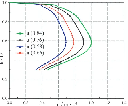
The effect of stationary bed on the velocity profiles is illustrated in figure 2 for different flow ratesQ. The mea-sured velocity profiles were asymmetrical, maximum ve-locity values were at distance abouth=23 mm above the pipe invert. The velocity gradient was steeper in the lower part of the profile and local velocities near the stationary bed (fromh=9 to 12 mm) were practically equal zero due to the high value of the bed roughness.

3 Mathematical model

The ﬂow ﬁeld is described by the incompressible Navier-Stokes equations

ρ_f

∂u

∂t +u· ∇u

=−∇p+μ∇2u,

with constant kinematic viscosityν. The fluid flow is driven by velocity profiles determined from experimental mea-surements which are illustrated in figure 2. The various pro-files are distinguished by the different flow rateQ.

Both the walls of the conduit and the surfaces of the moving particles are solid. The bed is semi-regularly cov-ered by stationary solid spherical particles. Thus, the no-slip boundary conditions (i.e., identification of the fluid ve-locity adjacent to the surface with the veve-locity of the sur-face) are defined for both cases as

(3)

u (0.84)

u (0.58) u (0.66)

h / D

u / m · s-1

u (0.76)

Fig. 2.The velocity profiles for different flow ratesQare depicted in various colors:Q=0.58 l s−1_{in blue,}_Q₌₀_._{66 l s}−1_{in red,}

Q=0.76 l s−1_{in black and}_Q₌₀_._{84 l s}−1_{in green. The e}_ﬀ_{ect of}

stationary bed made of spherical particles is manifested in shapes of the proﬁles.

whereurepresents ﬂow velocity andvstands for particle velocity in a boundary pointx_b.

Motion of solid particles in the ﬂow is determined by actions of body and hydrodynamic forces. The body force is represented by the gravitational forceFg. The hydrody-namic forces consists of the sum of the drag forceFd, the force due to added massF_mand the lift forceF_L, e.g., [8]. The resultant force also develops a torque on the particles which determines their angular velocitiesω.

Both the particle-bed and particle-particle collision mod-els are derived from impulse equations of the formm(v−

v) = J which use the impulse force Jas the measure of change of momentum (the quote mark distinguishes veloc-ities before and after collisions). It is supposed that colli-sions take place in a very short time and all external forces can be neglected.

If rotation is taken into account the corresponding im-pulse equation for the angular velocities before and after the collision reads asI(ω−ω) = rJt where I stands for momentum of inertia and Jt is the tangential component of the impulse force. The above relations enable to derive expressions for new velocities after collisions for both the particle-bed and particle-particle collisions, cf. [9–11]).

4 Numerical method

The numerical model of the above described system is based on the LBM approach. In the LBM the fluid is composed of fictive particles which propagate along the lattice links and interact in nodes. A fictive particle is represented by the particle distribution functionf(x,ci,t) which give probabil-ity of finding the fictive particle in a nodexwith a certain discrete velocityciin timet. Dynamics of fictive particles is described by the lattice Boltzmann equation

fi(x+ciΔt,t+Δt)− fi(x,t)=Γi,

where the termΓion the right-hand side represents a col-lision operator which is required to fulﬁll the ﬁrst law of

thermodynamics, i.e., in this case conservation of mass and momentum (Δtis the lattice time step). The simple and fre-quent choice is represented by the Bhatnagar-Gross-Krook (BGK) collision operator

Γ_i= 1_τ(f_ieq− fi). (1)

It expresses the tendency of the particle distributions fito local equilibriaf_ieqand the so called relaxation parameterτ expresses the rate of the tendency to the local equilibrium

f_ieq.

Macroscopic boundary conditions have to be expressed with the help of lattice numerical schemes which represent them on the microscopic level of the ﬁctive particles. For the no-slip boundary condition the so called bounce-back scheme is employed

fi(xb,t+1)= f−i(xb,t+1/2),

which consists in inversions of particle distributions along the directions incident to the boundary nodes, denoted by exchange i for −i. In the case of the moving surface the term corresponding to the exchange of momentum between ﬁctive particles and the moving macroscopic particle has to be added to the inverted distributions

fi(xb,t+1)= f−i(xb,t+1/2)+2

w_iρ(xb,t)

c2

s

(ci·v),

where wi represents weights of respective discrete veloc-ities c_i, ρis the local density and c2

s is the lattice sound speed, cf. [12]. Thus, the additional term represents the ac-tion of a macroscopic object on the ﬁctive particles, i.e., on the ﬂow.

The velocity proﬁles speciﬁed by experimental mea-surements are implemented by the Zou-He boundary scheme [13] as it allows to impose given velocityu(xin,t) or pres-sure p(xin,t) on the boundary. In this case, only the non-equilibrium parts of distributions fi−fieqare bounced-back in the normal direction with respect to the boundary.

In the LBM frame motion of macroscopic objects is ef-fect of interaction of ﬁctive particles with surfaces of these objects. More precisely, such a motion is caused by the mo-mentum transferΔpfrom the ﬁctive particles to the macro-scopic particles. Time rate of this momentum transferΔp/Δt

defines the hydrodynamic forces by which the flow acts on the objects. The hydrodynamic forces are then calcu-lated as a sum over momentum contributions from all fic-tive particles incident to the boundary nodes of the objects Fb =−Δp/Δtwhere

Δp=2c−i

fi(xb,t)−

w_iρ(xb,t)

c2

s

(ci·v)

,

cf. [14]. Another two contributions to the hydrodynamic forces comes from nodes covered or uncovered by motion of a particle. The impulse forceFcovexerted on the particle is given by momentum sum over covered nodes from the previous time step while the forceF_ucovgives the negative impulse force increment corresponding to momentum from uncovered nodes. The total hydrodynamic forces is then expressed as the sumFb+Fcov+Fun.

(4)

accuracy, is invariant under time reversal and has other fa-vorable global properties [15].

5 Simulation

In the last years a number of simulation tools based on the LBM have been developed. The various softwares diﬀer in the application domains, in the ways of implementation, in employments of various programming resources and in overall robustness of their design. To assess capacity of the LBM based simulations in comparison with the traditional CFD approaches in aspects of eﬃciency, accuracy and sta-bility validations against experiments or numerical meth-ods are performed.

The stability of the LBM simulations is endangered for processes characterized by high Reynolds numbers in which case the relaxation parameter tends to the critical valueτ→ 1/2 equivalent to the inviscid ﬂow. In this case the LBM becomes unstable because of incapability to dis-sipate the energy due to very large velocity gradients. The instability issues are eliminated by various approaches and extensions, e.g., the multi-relaxation time (MRT) method or the regularized LBM or the so called the entropic LBM. In the developed simulation the last mentioned modi-ﬁcation of the LBM is employed. Thus, if the parameter τin the BGK approximation (1) is replaced by the factor α/2τwhere the parameterαrepresents a non-trivial root of equation

H(fi+α(f_ieq− fi))=H(fi), (2) with the Boltzmann H-function of the form

H(f)= i

filn_wfi i ,

then the second thermodynamic law is supported in the col-lision process, i.e., the entropy cannot decrease in the pro-cess. It results in unconditional stability of the method – even for high Reynolds number cases – while still retain-ing its locality and eﬃciency (Karlin et al., 2002, 2006 [16, 17]).

However, calculation of the parameterαin each (poten-tially disruptive) node means solving the non-linear equa-tion (2). This equaequa-tion is usually solved by combinaequa-tion of the bisection method and the Newton method. The ﬁrst method assumes that the interval inside which a solution exists is known while in the second method a suﬃciently closed estimate to the solution should be known. Neither of them is trivial.

The upper estimate of theαmaxparameter can be easily found as the minimal solution to the equations

fi+α(fieq− fi)=0,

where f_ieq− fi <0, which guarantees positivity of the par-ticle distribution in the node. The lower estimateα_min> 0 can be computed from a rather complicated relation deﬁned in [18]. In the developed simulation the Newton method is employed where the upper estimateαmax plays the role of the starting value as it is eﬃcient and preserves stability. If the calculation of theαdoes not converge to the solution of Eq. (2) then it is assumed that the valueαmaxtakes the role of the parameter α. To eliminate computational demands

the parameterαis evaluated only in nodes exceeding a tol-erance value for the deviation|(f_ieq− fi)/fi|<10−2, i.e., in nodes with large deviations of the population fifrom local equilibrium f_ieq.

The computational domain is covered by ﬁxed rectan-gular lattice with 320 thousands of nodes and local opera-tions over all nodes are parallelized. Thus parallelization of computations is employed especially in the cases of evalu-ations of distribution functions fiand calculations of their moments (densityρand velocityu).

Parallelization of computations is provided by employ-ment of the CUDA GPU computing technology within the MATLAB environment (and the associated Parallel Com-puting Toolbox). It means that all ﬁeld quantities are trans-ferred to the GPUs where operations are performed on them. The MATLAB environment is chosen partly for easy im-plementation of mathematical functions and structures and partly for the possibility of collective applications of oper-ations over all nodes.

The possibility of straightforward parallelization of the LBM simulations yields considerable advantage from the point of efficiency. On the other side, the fact that the lattice grid is fixed brings substantial increase in computational demands in the case of extensive refinement. This problem can be resolved by employing adaptive meshes in regions with significant velocity gradients, e.g., [19].

6 Results

For each glass ball-mixture ﬂow rate (Q=0.58, 0.66, 0.76, and 0.84 l s−1_{) one representative trajectory of an}

individ-ual particle is chosen – from a number of observed trajecto-ries, see in [1] – and compared to the path of the simulated particle. As just trajectories without mutual particle colli-sions were experimentally observed it can be assumed that motion of simulated particles consists mainly of free trans-lational and rotational motion and collisions with the bed.

Simulation of particle motion is evaluated in a domain of the length l = 80 mm and heighth = 40 mm which corresponds to the part of the optical box where the parti-cle trajectories were observed. The measured velocity pro-files are used for generation of the flow within the domain. Specifically, the profiles are induced at the inlet of the sim-ulated region and let to develop above the rough bed. Into such a fully developed flows the particles are released from experimentally obtained initial positions (x0, y0) with

ini-tial velocities (v_x0, vy0).

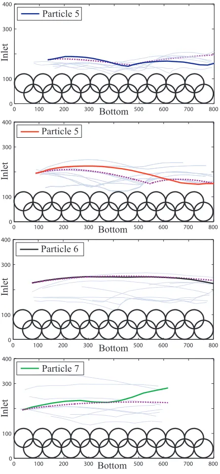
One experimental trajectory is chosen for each veloc-ity profile and it is compared with the corresponding sim-ulated trajectory. The couples of trajectories are drawn in Figs. 3 with respect to the length and height of the domain expressed in lattice space units. In the most upper figure the two trajectories – experimental and simulated – for the flow rateQ= 0.58 l s−1_{depart in the end of the examined}

domain. The second couple of trajectories for the ﬂow rate

Q= 0.66 l s−1 _{varies in the location of the collision with}

the bed. In the third case, for the ﬂow rateQ= 0.76 l s−1_,

the particles do not collide with the bed and they are al-most identical. Finally, the particles conveyed by the ﬂow withQ= 0.84 l s−1_{diverge at the outﬂow of the observed}

domain.

(5)

rea-0 100 200 300 500 600 700 800 0

100 300 400

Bottom

Inlet

Particle 5

0 100 200 300 500 600 700 800 0

100 300 400

Bottom

Inlet

0 100 200 300 500 600 700 800 0

100 300 400

Bottom

Inlet

Particle 6

0 100 200 300 500 600 700 800 0

100 300 400

Bottom

Inlet

Particle 7

Fig. 3. Comparisons of experimental and simulated trajecto-ries. The highlighted curves represent the compared trajectotrajecto-ries. Specifically, the purple/dashed ones stand for the simulated tra-jectories while the experimental tratra-jectories are drawn in color matching the velocity profiles in figure 2. From top to bottom fig-ures correspond to the flow rates in orderQ=0.58 l s−1_,

Q=0.66

l s−1_,

Q=0.76 l s−1_and

Q=0.84 l s−1_{. In the background other}

measured trajectories of particles with diﬀerent initial values can be seen depicted as tiny curves of an opaque color.

sons which can cause these diﬀerences. First of all, the ex-perimental particles are conveyed in the three-dimensional pipe while the developed simulation evaluates trajectories in the two-dimensional domain. Thus possibility of com-parison of experimental and simulated trajectories consists in assuming that transversal velocities of the particles are more or less insigniﬁcant. However, it is obvious that to de-termine particle trajectories more properly lateral motion must be taken into account and it is necessary to introduce the third dimension into the simulation.

Another cause of discrepancies can be the fact that ar-rangements of the stationary particles in the experiment are not quite well deﬁned. Irregular layout pattern can be re-solved by employment a random number generator used to pick out one location from all possible contact points [10]. However, from the shapes of some experimental trajecto-ries it can be seen that there are missing stationary particles in the higher level of the bed. In contrast, in the simulation a ﬁxed layout pattern and unchanging height of the bed (i.e., made of two layers) is assumed.

Another problem is represented by the way of release of the simulated particle into the ﬂow. Even if the parti-cle is placed in the corresponding initial position with the right initial velocity in the fully developed ﬂow its inser-tion in the domain induces unphysical disturbances at least in the start of the motion. This problem can be partly elimi-nated by introducing periodic boundary conditions through which the particle can enter the domain repeatedly.

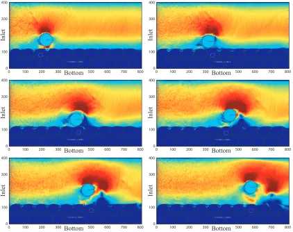
Finally, for illustration six snapshots of the instanta-neous flow field are shown in figure 4. It represents one of visual outputs of the developed simulation and should demonstrate the capability of the LBM to simulate both the particle motion and the fluid flow.

7 Conclusions

The LBM based simulation is developed to model particle motion in the water flow in the closed horizontal conduit. The simulation evaluates both the particle motion and ve-locity field of the flow. As the process is characterized by a high Reynolds number (up to 105) the entropic extensions of the LBM is employed to guarantee stability of compu-tation. Enhancement of computational resources is reached by parallelization of computations using the CUDA GPU technology. Assessment of accuracy of the used numerical approach is achieved by comparison of outputs of experi-mental measurements with results of the developed simu-lation.

It is shown that the compared – experimental versus simulated – trajectories given by identical initial values are quite similar though there are diﬀerences which can be caused by various reasons. In the simulation section 5 and the re-sult section 6 a number of problems is addressed. Each of them has to be solved to obtain an accurate, stable and eﬃ -cient simulation.

Firstly, as the entropic extension of the LBM depends largely on the correctness of the calculated valueαits cal-culation must be improved in such a way that it will be both sufficiently accurate and efficient. This can be reached by the modification of both the numerical method and its implementation.

For the second the simulation must be rewritten for three-dimensional domain as this inﬂuences the processes fundamentally though such a transformation yields increase of computational demands and additional implementation issues.

(6)

0 100 200 300 500 600 700 800 0

100 300 400

Bottom

Inlet

0 100 200 300 500 600 700 800 0

100 300 400

Bottom

Inlet

0 100 200 300 500 600 700 800 0

100 300 400

Bottom

Inlet

0 100 200 300 500 600 700 800 0

100 300 400

Bottom

Inlet

0 100 200 300 500 600 700 800 0

100 300 400

Bottom

Inlet

0 100 200 300 500 600 700 800 0

100 300 400

Bottom

Inlet

Fig. 4.Six snapshots of the instantaneous flow field are shown. They illustrate both the particle motion and the fluid flow as evaluated in a unique computational frame of the developed LBM based simulation. The first three figures depict conditions before a collision while the last three figures represent situations after the collision.

Further efficiency improvements in the algorithm and its parallelization will enable to simulate particle-fluid sys-tems at the particle scale and thus can help to understand better the underlying particle-fluid dynamics. For exam-ple, in the considered process high level turbulence with large eddies along the bed influences the particle motion mode due to intensive mutual interactions of particles and the flow (and particle-wall collisions). Such a simulation tool could provide quantitative data for turbulence model-ing difficult to obtain experimentally.

Acknowledgements

The support under the project No. P105/10/1574 of the GA CR and RVO: 67985874 of the Academy of Science of the Czech Republic is gratefully acknowledged.

References

1. P. Vlas´ak, B. Kysela, Z. Ch´ara, Part. Sc. Tech. 32, (2013) 179-185

2. U. Frisch, B. Hasslacher, Y. Pomeau, Phys. Rev. Lett. 56, (1986) 1505-1508

3. G. R. McNamara, G. Zanetti, Phys. Rev Lett.61, 1988 2332-2335

4. S. Succi, The lattice Boltzmann equation for ﬂuid dy-namics and beyond(Clarendon, Oxford, 2001)

5. X. He, L.-S. Luo, J. Stat. Phys.88, (1997) 927-944 6. Z. Yu, L. S. Fan, Particuology8, (2010) 539-543 7. P. Vlas´ak, B. Kysela, Z. Ch´ara, J. Hydrol. Hydromech.

60, (2012) 115-124

8. P. L. Wiberg, J. D. Smith, J. Geophys. Res.90(1985) 7341-7354

9. W. Czernuszenko, Arch. Hydro-Eng. Env. Mech., 56 (2009) 101-120

10. N. Lukerchenko, Z. Ch´ara, P. Vlas´ak, J. Hydraul. Res. 44, (2006) 70-78

11. N. Lukerchenko, N., Piatsevich, S., Ch´ara, Z. and Vlas´ak, P., J. Hydrol. Hydromech.57(2009) 100-112 12. A. J. C. Ladd, J. Fluid Mech.271, (1994) 311-339 13. Q. Zou, X. He, Phys. Fluids9, (1997) 1591

14. C. K. Aidun, Y. Lu, E. J. Ding, J. Fluid. Mech. 373, (1998) 287-311

15. M.P. Allen, D. J. Tildesley, Computer Simulation of Liquids(Clarendon, Oxford, 1987)

16. S. Ansumali, I. V. Karlin, J. Stat. Phys. 107, (2002) 291-308

17. S. S. Chikatamarla, S. Ansumali, I. V. Karlin, Phys. Rev. Lett.97, (2006) 010201

18. A. N. Gorban, I. V. Karlin, V. B. Zmievskii, T. F. Non-nenmacher, Physica A231, (1996) 648-672