Article
Simulation Analysis of Capacitance Method in Two-Phase
Flow Concentration Measurement by Coupled Fields
Xiaoxin Wang 1, Hongli Hu 1,*, Lin Li 1 and Bo Wang 2
1 State Key Laboratory of Electrical Insulation and Power Equipment, Xi’an Jiaotong University,
Xi’an 710049, China; [email protected] (X.W.); [email protected] (L.L.)
2 Institute of Geophysical Instrument, Xi’an Research Institute of China Coal Technology &
Engineering Group Corp, Xi’an 710077, China; [email protected] * Correspondence: [email protected]
Abstract: This paper proposed three-dimensional numerical simulation method by coupling
of electrostatic and fluid fields to evaluating the performance of electrical sensor in the concentration measurement of gas/solid two-phase flow. Compared with the static numerical simulation, this real-time dynamic 3-D simulation method can research on a designed capacitance sensor combining the dynamic characteristics of the two-phase flows for concentration measurement. Several fluid-electrostatic models of transmission pipes with different sensor structures are built. Under different test positions and different particle concentrations, the flow characteristics and the corresponding electric signals can be obtained, and the correlation coefficient between the concentration values and the capacitance values are used for performance evaluation of the sensors. The effects of flow regimes on concentration measurement are also been investigated in this paper. To validate the results of simulation, an experimental platform with horizontal straight pipe for phase volume concentration measurement of solid/air two-phase flow is built, and the experimental results agree well with simulation conclusions. The simulation and test results show that the coupling models can give constructive reference opinions for the sensor design and collection of installation position in different transmission pipelines, which are very important for the practical process of pneumatic conveying system.
Keywords: 3-D fluid-electrostatic coupling field; electrical sensor performance; concentration
measurement; gas/solid two-phase flow
1. Introduction
Pneumatic conveying of solid particles exists widely in thermal power, steel smelting, chemical and food industry. The accurate measurement of gas/solid flow parameters (flow regime, velocity, phase concentration, mass flow, etc.) is of great importance in reducing air pollution and pipe wearing as well as improving product quality and production efficiency [1,2]. Moreover, phase concentration is a key parameter among these flow parameters. Capacitance method as one of the most promising technology for two-phase flow parameter measurement has the advantages of simple construction, involving nuclear radiation, high sensitivity, economical and non invasion. Electrodes mounted on the transmission pipeline, when the flow passes through the sensitive space of the mounted sensor, the equivalent dielectric constant of this section will changes, then the mean capacitance value of sensing electrodes will changes, too [3]. Several configurations of capacitance sensors have been proposed and analyzed, i.e., concave, helical, and ring structures [4-7]. Static simulation of the electrostatic field is usually applied to investigate the performance of a designed capacitance sensor [8].
the performance of a designed surface electrode systems with different structural parameters, and a optimum electrode designs were proposed with high sensitivity and low deviation from linearity to different flow patterns. According to the poor measuring sensitivity and sensing field sensitivity uniformity of the capacitance sensor, Wang X X et al. [10] reported a method combining 2-D ANSYS finite element analysis with orthogonal experiment to investigate the performance of 3 kinds of capacitance sensors, and their variance analyses were done on the test results. The optimum combination schemes were obtained by analyzing and comparing the effects of various parameters on different capacitance sensors. Yang W Q et al. [11] proposed a 2-D simulation model of ECT sensor by coupling fluid field and electrostatic field to investigate the performance of the ECT sensor and image reconstruction algorithm. By using this computational simulation method of coupled field, the time-varying capacitance values and permittivity distributions can be obtained. However, there are little real-time dynamic 3-D simulation researches on a designed capacitance sensor combining the dynamic characteristics of the two-phase flows for concentration measurement. Moreover, the study object in previous research is usually a section of straight pipe [12,13]. However, in the practical process of pneumatic conveying system, curving pipe, variable-diameter pipe and other special pipe structures are also commonly existed in transmission pipelines, and the flow characteristics around these special pipes are different from each other [14,15,16], so the performance researches of the sensors installed around these special pipes are also important.
In this paper, by coupling of electrostatic and fluid fields, 3-D coupling models of straight pipe, curving pipe and variable-diameter pipes with 3 different sensor structures for concentration measurement are studied and the concentration distribution and the corresponding capacitance values of sensing electrodes can be obtained with varying time. The flow patterns and the corresponding sensor signals can be obtained and analyzed under different sensor structures, different installation positions and different particle concentrations. The correlation coefficient between the concentration values and the capacitance values are calculated to evaluate the performance of the sensors. To validate the simulation results, an experimental platform with horizontal straight pipe for phase volume concentration measurement of solid/air two-phase flow is built and used for experimental studies. The main purpose of this article is to demonstrate the effectiveness of the coupling model, and investigate the corresponding relationship between the flow characteristics and the electric signals, then provide an effective approach to design and evaluate different kinds of electronic sensors in a practical process of pneumatic conveying system.
2. Coupling model
In electrostatic field, according the Possion’s equation and the Dirichlet boundary conditions [17]
−∇ =
= ⋅ ∇
V E
D 0
and D=ε0εrE , (1)
where D is the electric displacement field, E is the electric field intensity distribution, V is the electric potential, ε0is the permittivity of vacuum andεris the relative permittivity of the mixture.
In two-phase flow field, the Euler-euler transient model is used to model the real-time dynamics of gas-solid flow. The model is expressed by the continuity equation and momentum equation:
Continuity equation,
= ⋅
∇ + ∂
∂
= ⋅
∇ + ∂
∂
0 ) (
) (
0 ) (
) (
d d d d
d
c c c c
c
u t
u t
φ ρ φ
ρ
φ ρ φ
ρ
whereφc and φdare the holdup of continuous phase and dispersed phase, φc =1−φd, ρcand
d
ρ are the concentrations of the continuous phase and dispersed phase, and ucand ud are
the velocities of the continuous phase and dispersed phase. Momentum equation, + + + ⋅ ∇ + ∇ − = ⋅ ∇ + ∂ ∂ + + + ⋅ ∇ + ∇ − = ⋅ ∇ + ∂ ∂ d F d d m F g d d d d p d d u d u t d u d d c F c c m F g c c c c p c c u c u t c u c c φ ρ φ τ φ φ φ ρ φ ρ φ τ φ φ φ ρ , ) ( I ) ( , ) ( I ) (
, (3)
where pis the mixed phase pressure, τ (τcorτd) is the viscous stress tensors, gis the gravitational acceleration, Fm(Fm,corFm,d) is the interaction force between the two phase and
F(FcorFd) is any additional volume force [18, 19].
Where ∇ + ∇ − ∇⋅ = ∇ + ∇ − ∇⋅ = I ) ( 3 2 ) ( I ) ( 3 2 ) ( d T d d d d c T c c c c u u u u u u μ τ μ τ (4) c
μ andμd(Pa.s)are the dynamic visosity of continuous phase and dispersed phase. In the coupled model of this article,Fis the electric force. The electric force can be expressed as [20]:
T
F =∇⋅ , (5)
) 2
1
( , 2
0
, EE E
Ti j =ε εr i j− δi j , (6)
j i,
δ is the Kronecker delta and i, j represent the components in the coordinate system.
− − − − − − = ) ( 2 1 ) ( 2 1 ) ( 2 1 2 2 2 2 2 2 2 2 2 0 y x z z y z x z y z x y y x z x y x z y x r E E E E E E E E E E E E E E E E E E E E E
T ε ε (7)
Relative permittivity of the mixtureεr can be defined by the internally defined solid-phase volume fraction, εr =εdφd +εc(1−φd) , where εd and εc are the relative permittivities of solid and gas.
3. Coupling simulation
3.1 Simulation condition
Table 1 Simulation condition (a) Solid-gas flow field
Parameters Value Description
c
ρ (kg/m3) 1.2 Density, continuous phase
d
ρ (kg/m3) 900 Density, dispersed phase
c
μ (Pa.s) 1.8*e-5 Dynamic viscosity, continuous phase
d
d (m) 5.4*e-5 Diameter, dispersed phase
max
φ 0.62 Maximum packing concentration
α (o) 60 Angle between inlet 1 and inlet 2
0 c
u (m/s) 2 velocity ( inlet 1), continuous phase
(b) Electrostatic filed
Parameters Value Description
c
ε 1 Relative permittivity, continuous phase
d
ε 4.3 Relative permittivity, dispersed phase
A (V) 3.3 Amplitude of excitation signal
Table 2 Parameters of the 3 capacitive sensors
Parameters Values Values Values
Electrodes number 2 4 8
Electrode opening angle 120° 60° 30°
Electrodes length (mm) 100 100 100
3.2 The performance of 3 sensors on different transmission pipelines model
In the practical process of pneumatic conveying system, three pipe structures, straight pipe, curving pipe and variable-diameter pipe, are three common structures in transmission pipelines. Under the three coupling fluid-electrostatic models, the performance of concentration measurement with 3 different sensors are investigated in this paper.
(a) Straight pipe
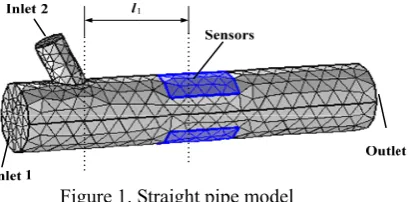
Figure 1. Straight pipe model
Figure 1 is the discretized model of the straight pipe and the sensors. The diameter of
l1(mm) T=0.2s T=0.4s T=0.8s T=1.2s T=2s T=3s
50
100
150
200
250
300
Figure 2. The volume fraction distribution of dispersed phase
In the case of constant input conditions, it can be seen from Figure 2 that the flow patterns are unstable before 0.8s and they are became relatively stable after 1.2s, which means that it needs some transient time to achieve stable flow pattern. The transient time is related to the velocity of carrier air in inlet1, for example: v=8m/s the transient time is about 0.7s, and
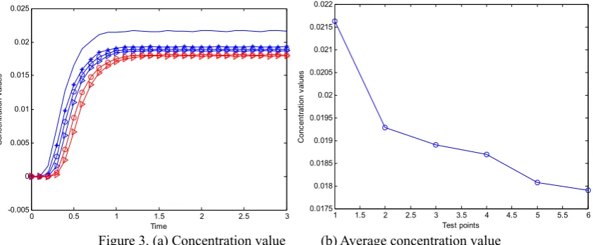
v=18m/s the transient time is about 0.5s. Moreover, with the increase of l1 the flow pattern is from non-homogeneous flow (e.g. l1=50mm, 100mm, 150mm) to relatively homogeneous flow (e.g. l1=200mm, 250mm, 300mm). Figure 3(a) shows 31 concentration values (collected one value at every 0.1s from 0s to 3s) of the dispersed phase at 6 different cross-sectional positions. And the average concentration values under the stable flow pattern condition (from 1.2s to 3s) of the 6 positions are drawn in Figure 3(b).
0 0.5 1 1.5 2 2.5 3
-0.005 0 0.005 0.01 0.015 0.02 0.025
Time
C
onc
en
tr
at
io
n v
al
ues
1 1.5 2 2.5 3 3.5 4 4.5 5 5.5 6 0.0175
0.018 0.0185 0.019 0.0195 0.02 0.0205 0.021 0.0215 0.022
Test points
C
onc
en
tr
at
io
n v
al
ues
As shown in Figure 3(a) and (b), with the increase of l1there is a decreasing trend of the concentration variations. The average concentration value at l1=50mm has maximum difference compared with others, and the differences between the remaining 5 average concentration values are not big.
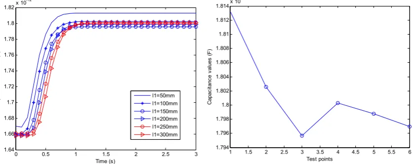
For the fluid-electrostatic model, the corresponding capacitance value of the electrode pairs can be obtained in the dynamic flow process. Figures 4, 5 and 6 show the corresponding capacitance values and their variations trend at 6 different installed positions of the sensors with 2-electrode, 4-electrode and 8-electrode, respectively.
0 0.5 1 1.5 2 2.5 3
1.64 1.66 1.68 1.7 1.72 1.74 1.76 1.78 1.8 1.82x 10
-12 Time (s) C apac itanc e v al ues (F ) l1=50mm l1=100mm l1=150mm l1=200mm l1=250mm l1=300mm
1 1.5 2 2.5 3 3.5 4 4.5 5 5.5 6 1.794 1.796 1.798 1.8 1.802 1.804 1.806 1.808 1.81 1.812 1.814x 10
-12 Test points C apac itanc e v al ues ( F )
Figure 4. (a) Capacitance values with 2-electrode (b) Capacitance variations trend with 2-electrode
0 0.5 1 1.5 2 2.5 3
3.05 3.1 3.15 3.2 3.25 3.3 3.35 3.4 3.45x 10
-12 Time (s) C apac itan ce v al ues ( F ) l1=50mm l1=100mm l1=150mm l1=200mm l1=250mm l1=300mm
1 1.5 2 2.5 3 3.5 4 4.5 5 5.5 6 3.34 3.35 3.36 3.37 3.38 3.39 3.4 3.41 3.42 3.43 3.44x 10
-12 Test points C apa ci ta nc e v al ue s ( F )
Figure 5. (a) Capacitance value with 4-electrode (b) Capacitance variations trend with 4-electrode
0 0.5 1 1.5 2 2.5 3
6.7 6.8 6.9 7 7.1 7.2 7.3 7.4 7.5 7.6x 10
-12 Time (s) C apa ci tanc e v al ues (F ) l1=50mm l1=100mm l1=150mm l1=200mm l1=250mm l1=300mm
1 1.5 2 2.5 3 3.5 4 4.5 5 5.5 6 7.4 7.42 7.44 7.46 7.48 7.5 7.52 7.54 7.56 7.58
7.6x 10 -12 Test points C ap ac itanc e v al ue s ( F )
By comparing Figures 4(a), 5(a) and 6(a) with Figure 3(a), all the curves tend to be stable after a rising stage at about 1s. The curve variations tendencies in Figures 4(b) and 5(b) are similar with that of in Figure 3(a), while the Figure 6(a) is not. Here, use the correlation coefficient to evaluate the performance of the sensors.
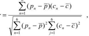
The correlation coefficient (r) can be expressed as:
= =
=
− −
− −
= 6
1
6
1
2 2
6
1
) ( ) (
) )( (
n n j n
n
n n
c c p
p
c c p p
r , (8)
Where p and c are the average concentration and capacitance values under the stable flow pattern condition of the 6 positions of pipe. Here, r represents the correlation coefficient between the concentration values and the measured capacitance values by 2-electrode, 4-electrode and 8-electrode and they are shown in Table 3.
Table 3 Correlation coefficient
Sensor 2-electrode 4-electrode 8-electrode
r 0.9241 0.8189 -0.3878
Table 3 shows that the capacitance values obtained by 2-electrode have the best correlation relation (r=0.9241) with the concentration values, and next is 4-electrode (r=0.8189), and the worst is 8-electrode (r=-0.3878). From Figures 3 to 6, for the same concentration variations, the corresponding capacitance ranges are 1.7956*10-12- 1.8131*10-12F, 3.3417*10-12-3.4386*10-12F and 7.4021*10-12- 7.5853*10-12F for 2-electrode, 4-electrode and 8-electrode, respectively. So with the increase of the electrode number, the sensitivity of the capacitance measurement is improved and the measurement range is also rose.
Considering the above factors, both the 2-electrode and 4-electrode can be chosen for concentration measurement of solid-gas two-phase flow in this straight pipe, and they should be further selected according to the actual situation.
Moreover, for the 6 groups stable flow patterns in Figure 2, they could be divided into two kinds of flow patterns (kind 1: l1=50mm, 100mm, 150mm; kind 2: l1=200mm, 250mm, 300mm). Combined with Figures 2, 3(b), 4(b) and 5(b), we can found that the capacitance values and concentration values have very good correlation relation under the same kind of flow pattern. However, when the differences of flow patterns are varying widely, the correlation relation will be decreased, e.g. l1=150mm and l1=200mm, where the capacitance values are increased with a decrease of concentration values. So it can be conclude that the variations of the flow regimes affect the concentration measurement of two-phase flow by capacitance sensors.
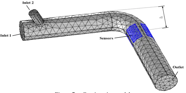
Figure 7. Curving pipe model
Figure 7 is the discretized model of the curving pipe and the sensors. A curving pipe is added behind the original straight pipe. The angle of turning circleα is 90o, and R/D=2 where R is the radius of turning circle and D is the pipe diameter. l2 is the distance between the straight pipe and the center of sensors. The sensors are installed on 6 different positions
l2=150mm, 200mm, 250mm, 300mm, 350mm, 400mm, respectively, and the operational cycle for each position is 3s. The volume fraction distribution of dispersed phase on these cross sections in Figure 8 are captured at 0.3s, 0.6s, 0.9s, 1.2s, 2s, and 3s, respectively, and the color ranges of all the images are set to the same.
l2(mm) T=0.3s T=0.6s T=0.9s T=1.2s T=2s T=3s
150
200
250
300
350
400
As shown in Figure 8, under the constant input conditions it is need about 1.2s to achieve stable flow patterns which are close to laminar flow. Moreover, with the increase of l2 the degree of particles' aggregation is reduced and the distributions of particles gradually become homogeneous. Figure 9(a) shows the concentration values (collected one value at every 0.1s from 0s to 3s) of the dispersed phase at 6 different cross-sectional positions. And the average concentration values under the stable flow pattern condition (from 1.2s to 3s) of the 6 positions are drawn in Figure 9(b).
0 0.5 1 1.5 2 2.5 3
-5 0 5 10 15 20x 10
-3
Time (s)
C
onc
ent
ra
tion v
al
ues
l2=150mm l2=200mm l2=250mm l2=300mm l2=350mm l2=400mm
1 1.5 2 2.5 3 3.5 4 4.5 5 5.5 6 0.0158
0.016 0.0162 0.0164 0.0166 0.0168 0.017 0.0172 0.0174 0.0176
Test points
C
onc
ent
ra
tion v
al
ues
Figure 9. (a) Concentration values from 0s to 3s (b) Average concentration value
As shown in Figure 9, for l2=150mm, 200mm, 250mm, 300mm, with the increase of l2 there is a decrease trend of the average concentration. While for l2=350, 400mm, the variation trend is different.
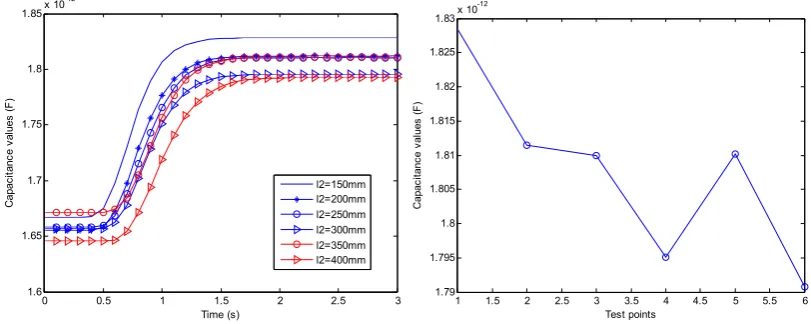
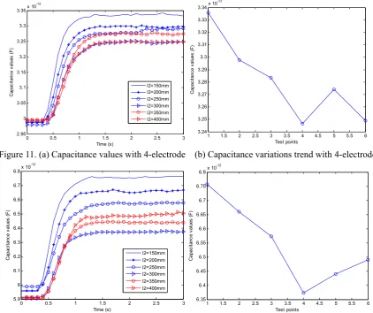
For the fluid-electrostatic model, the corresponding capacitance value of the electrode pairs can be obtained in the dynamic flow process. Figures 10, 11 and 12 show the corresponding capacitance values and their variations trend at 6 different installed positions of the sensors with 2-electrode, 4-electrode and 8-electrode, respectively.
0 0.5 1 1.5 2 2.5 3
1.6 1.65 1.7 1.75 1.8 1.85x 10
-12
Time (s)
C
apa
ci
tanc
e v
al
ue
s
(F
)
l2=150mm l2=200mm l2=250mm l2=300mm l2=350mm l2=400mm
1 1.5 2 2.5 3 3.5 4 4.5 5 5.5 6 1.79
1.795 1.8 1.805 1.81 1.815 1.82 1.825
1.83x 10
-12
Test points
C
ap
ac
itanc
e v
al
ue
s (
F
)
0 0.5 1 1.5 2 2.5 3 2.95
3 3.05 3.1 3.15 3.2 3.25 3.3 3.35x 10
-12
Time (s)
C
apa
ci
ta
nc
e v
al
ue
s (F
)
l2=150mm l2=200mm l2=250mm l2=300mm l2=350mm l2=400mm
1 1.5 2 2.5 3 3.5 4 4.5 5 5.5 6 3.24
3.25 3.26 3.27 3.28 3.29 3.3 3.31 3.32 3.33 3.34x 10
-12
Test points
C
apac
itanc
e v
al
ues
(
F
)
Figure 11. (a) Capacitance values with 4-electrode (b) Capacitance variations trend with4-electrode
0 0.5 1 1.5 2 2.5 3
5.9 6 6.1 6.2 6.3 6.4 6.5 6.6 6.7 6.8x 10
-12
Time (s)
C
ap
ac
itanc
e v
al
ue
s (F
)
l2=150mm l2=200mm l2=250mm l2=300mm l2=350mm l2=400mm
1 1.5 2 2.5 3 3.5 4 4.5 5 5.5 6 6.35
6.4 6.45 6.5 6.55 6.6 6.65 6.7 6.75
6.8x 10 -12
Test points
C
apac
itanc
e v
al
ues
(F
)
Figure 12.(a) Capacitance values with 8-electrode (b) Capacitance variations trend with8-electrode
By comparing Figures 10(a), 11(a) and 12(a) with Figure 9(a), all the curves tend to be stable after a rising stage at about 1.2s. For the curving tube model, the correlation coefficients between the concentration values and the measured capacitance values of 2-electrode, 4-electrode and 8-electrode can be calculated by equation (8) and the results are shown in Table 4.
Table 4 Correlation coefficient
Sensor 2-electrode 4-electrode 8-electrode
r 0.8913 0.9326 0.8694
Table 4 shows that the capacitance values obtained by the three sensor structures all have good correlation relations with the concentration values, and 4-electrode has the best correlation relation r=0.9326, and the next is 2-electrode r=0.8913, and the last is 8-electrode
r=0.8694.
As shown in Figures 9 to 12, for the same concentration variations, the corresponding capacitance ranges are 1.7907*10-12-1.8283*10-12F, 3.2467*10-12-3.3357*10-12F and 6.3730*10-12- 6.7577*10-12F for 2-electrode, 4-electrode and 8-electrode, respectively. Which means that with the increase of the electrode number, the sensitivity of the capacitance measurement is improved and the measurement range is also increased. Considering the above factors, all the three sensor structures can be used for concentration measurement of the solid-gas two-phase flow in curving pipe, and they could be further selected according to the actual situation.
and l2=200mm have slight differences with other 4 groups, and as shown in Figures 9(b), 10(b) and 11(b) the correlation relation of the 4 groups are better than that of l2=150 and l2=200 mm. So it can be conclude that the variation of the flow regimes affects the concentration measurement of solid-gas two phase flow in curving pipe.
(c) Variable-diameter pipe
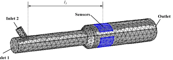
Figure 13. Variable-diameter pipe model
Figure 13 is the discretized model of the variable-diameter pipe and the sensors. A variable-diameter pipe with diameter 160mm is added behind the original straight pipe. The angle of variable-diameter is 45o. l3 is the distance between the inlet 2 and the center of sensors. The sensors are installed on 6 different positions l3=580mm, 630mm, 680mm, 730mm, 780mm and 830mm, respectively, and the operational cycle for each position is 3s. The volume fraction distribution of dispersed phase on these cross sections in Figure 8 are captured at 0.3s, 0.6s, 0.9s, 1.5s, 2s, and 3s, respectively, and the color ranges of all the images are set to the same.
l3(mm) 0.3s 0.6s 0.9s 1.5s 2s 3s
580
630
680
730
780
830
Figure 14. The volume fraction distribution of dispersed phase
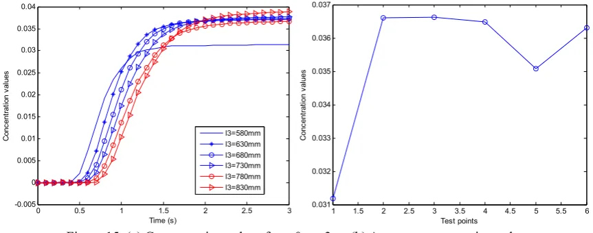
transmission pipe. Figure 15(a) shows the concentration values (collected one value at every 0.1s from 0s to 3s) of the dispersed phase at 6 different cross-sectional positions. And the average concentration values under the stable flow pattern condition (from 2s to 3s) of the 6 positions are drawn in Figure 15(b).
0 0.5 1 1.5 2 2.5 3
-0.005 0 0.005 0.01 0.015 0.02 0.025 0.03 0.035 0.04 Time (s) C on cent ra tion v al ues l3=580mm l3=630mm l3=680mm l3=730mm l3=780mm l3=830mm
1 1.5 2 2.5 3 3.5 4 4.5 5 5.5 6 0.031 0.032 0.033 0.034 0.035 0.036 0.037 Test points C onc ent rat io n v al ues
Figure 15. (a) Concentration values from 0s to 3s (b) Average concentration value
As shown in Figure 15, for l3=630mm, 680mm, 730mm and 830mm, the average concentration are basically the same. While the concentration of l3=580mm has a big difference with the others, and the difference of l3=780mm is relatively small.
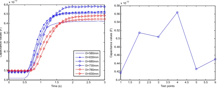
For the coupled model, the corresponding capacitance values of the electrode pairs can be obtained in the dynamic flow process. Figures 16, 17 and 18 show the corresponding capacitance values and the variations trend of average capacitances at different installed positions of the sensors with 2-electrode, 4-electrode and 8-electrode, respectively.
0 0.5 1 1.5 2 2.5 3
1.75 1.8 1.85 1.9 1.95
2x 10 -12 Time (s) C apac itanc e v al ue s ( F ) l3=580mm l3=630mm l3=680mm l3=730mm l3=780mm l3=830mm
1 1.5 2 2.5 3 3.5 4 4.5 5 5.5 6 1.85
1.9 1.95
2x 10 -12 Test points C ap aci ta nc e va lu es ( F )
Figure 16. (a) Capacitance values with 2-electrode (b) Capacitance variations trend with2-electrode
0 0.5 1 1.5 2 2.5 3
3.1 3.15 3.2 3.25 3.3 3.35 3.4 3.45 3.5 3.55x 10
-12 Time (s) C apa ci ta nc e v al ues (F ) l3=580mm l3=630mm l3=680mm l3=730mm l3=780mm l3=830mm
1 1.5 2 2.5 3 3.5 4 4.5 5 5.5 6 3.4 3.42 3.44 3.46 3.48 3.5 3.52x 10
-12 Test points C ap ac itanc e v al ues ( F )
0 0.5 1 1.5 2 2.5 3 5.8
5.9 6 6.1 6.2 6.3 6.4 6.5 6.6x 10
-12
Time (s)
C
apac
ita
nc
e v
al
ue
s (
F
)
l3=580mm l3=630mm l3=680mm l3=730mm l3=780mm l3=830mm
1 1.5 2 2.5 3 3.5 4 4.5 5 5.5 6 6.4
6.42 6.44 6.46 6.48 6.5 6.52 6.54 6.56 6.58x 10
-12
Test points
Capac
itanc
e v
al
ues
(
F
)
Figure 18. (a) Capacitance values with 8-electrode (b) Capacitance variations trend with 8-electrode
As shown in Figures 15(a), 16(a), 17(a) and 18(a), all the curves tend to be stable after a rising stage at about 2s, which is kept consistent in Figure 14. For the variable-diameter pipe model, the correlation coefficient between the concentration values and the measured capacitance values by 2-electrode, 4-electrode and 8-electrode can be calculated using (8) and the results are shown in Table 5.
Table 5 Correlation coefficient
Sensor 2-electrode 4-electrode 8-electrode
r 0.9278 0.9843 0.6815
As shown in Table 5, the capacitance values obtained by 2-electrode and 4-electrode have better correlation relations with the concentration values than that by 8-electrode. Especially for 4-electrode, its correlation relation r can reach to 0.9843. As shown in Figures 15 to 18, for the same concentration variations, the corresponding capacitance ranges are 1.8745*10-12-1.9819*10-12F, 3.4045*10-12-3.5194*10-12F and 6.4169*10-12- 6.5638*10-12F for 2-electrode, 4-electrode and 8-electrode, respectively. So with the increase of the electrode number, the measurement range is increased but not very obvious. Considering the above factors, sensor structure with 4-electrode is the best choice for concentration measurement of the two-phase flow in this curving pipe model.
As shown in Figure 14, all the 6 groups stable flow patterns with different l3 are very similar. So combined with Figures 15 to 18, the influence of the flow regimes variation on the concentration measurement of solid-gas two-phase flow in this model is not distinct.
According to the above analysis, the measurement performances of different sensors can be evaluated by the coupling simulation models, and it is very meaningful to choose the appropriate sensors for the concentration measurement of the actual two-phase flow model. Moreover, we found that under the same simulation model the correlation relations between the capacitance and concentration values are affected by variations in the flow regimes. To further verify the conclusion, simulation experiments are carried out in the following sections to study the influence of flow regimes’ variations on concentration measurement.
3.3 Influence of flow regimes’ variation on the concentration measurement
pv Group1:eccentric flow Group2:laminar flow Group3:mixture
0.1
0.2
0.3
0.4
0.5
Figure 19 volume fraction distribution of dispersed phase
In Figure 19, the color ranges of the images are adjusted adaptively. All the flow patterns of group1 can be classified as a same type (eccentric flow) with different concentration values and the same to group2 (laminar flow). While for group3 the flow patterns are not belong to a same type. For 2-electrode sensor investigation, fitted equations of the three groups, which describe the relationships between the concentration values of dispersed phase and the capacitance values, and their corresponding parameters are shown in Table 6.
Table 6 Simulation test results with 2-electrode
Flow regime Group1 Group2 Group3
Fitted equation y=1.3156*109x-0.0021 y=1.1263*109x-0.0018 y=1.2446*109x-0.0020
Linearity(%) 0.9 0.11 3.7
Average relative
error ( Are %) 0.992 0.168 5.15
For the concentration measurement with 4-electrode sensor, the fitted equations of the three groups, and their corresponding parameters are shown in Table 7.
Table 7 Simulation test results with 4-electrode
Flow regime Group1 Group2 Group3
Fitted equation y=1.0904*109x-0.0032 y=6.9557*108x-0.0021 y=7.2536*108x-0.0022
Linear(%) 7.02 2.02 51.9
Average relative
error ( Are %) 4.606 2.418 32.42
(x (F) is the capacitance value, input , y is the solid-gas volume ratio.)
Compared Table 6 with Table 7, the measurement performance with 2-electrode are better than that with 4-electrode, which is consistent with the previous conclusions in Table 3. As shown in Table 6 and Table 7, the linearity values of Group3 are much higher than that of Group1 and Group2, which means that the linearity characteristic of Group3 is the worst. And the average relative errors of Group3 are 5.15% and 32.42% , which are much bigger than that of Group1 (0.992% and 4.606%) and Group2 (0.168% and 2.418%). So it can be conclude that for the same concentration measurement system the measurement characteristics with classified flow regimes are better than that of without classified flow regimes, which means that the concentration measurement by electrical method are affected by variations of the flow regimes.
4 experimental results
In order to validate the simulation results, an experimental platform with straight pipe for phase concentration measurement of pulverized coal/air two-phase flow is built and it is shown in Figure 20. It consists of five parts: carrier air supply part, feeding part, flow pattern generator, test part and collection part[22].
The gas and particles used in the experiment are gas and pulverized coal (PC). Set the supplier air velocity 18m/s, and feeding amount ranges from 12.82g/s to 54.22g/s for PC, according to the definition described in reference [22] of the relationship between the actual concentration of pulverized coal and the mass flow rate, the volume concentrations of pulverized coal range from 0.1006×0.1% to 0.4263×0.1%. The discharging amount of pulverized coal are adjusted by feeders, and they are regarded as the calibration values which determines the actual volumetric concentration of pulverized coal. The measuring section is a quartz glass pipe of length 1.20m, and its inner and outer diameters are 96mm and 100mm. The capacitance measuring circuit is a C/V (capacitance to voltage) conversion circuit, an excitation voltage with 1MHz frequency and 3.3V amplitude are used [23]. 2-electrode and 4-electrode are studied in experimental part, each electrode is scattered evenly around the insulating wall. A ring-shaped electrostatic sensor with axial length of 20mm is applied for flow regime identification [24]. The electrostatic signals are collected for flow pattern identification of the gas/solid two-phase flow [19]. The subband energies of the electrostatic signal Hilbert marginal spectra of different flow patterns are extracted by Hilbert-Huang transform(HHT), and the extracted features are used as inputs of the ELM (extreme learning machine) identification model, and the outputs are identified flow patterns [21].
uniform flow are generated by three different throttling devices [21].
Figure 20 Schematic diagram of a pneumatic conveying system
4.1 Calibration Tests
Under each known flow pattern, 10 capacitance values are measured for each of 10 concentrations and the 10 different concentrations are set by adjusting the feeding amount. Then the relationships between the capacitance values (average of the measured ten capacitance values) and the solid-gas volume concentration can be obtained, and their fitted equations and corresponding parameters with 2-electrode and 4-electrode are shown in Table 8 and 9. x (pF) is the capacitance value, y is the solid-gas volume ratio.
Table 8 Calibration test results under known flow pattern with 2-electrode
Flow regime Core flow Stratified flow Uniform flow
Fitted equation y=4.8621x-6.7036 y=4.5419x-6.5985 y=4.5550x-6.6180
Linearity(%) 1.16 0.98 0.47
Table 9 Calibration test results under known flow pattern with 4-electrode
Flow regime Core flow Stratified flow Uniform flow
Fitted equation y=3.8133x-10.1937 y=2.8077x-7.5315 y=2.6657x-7.5467
Linearity(%) 7.55 3.7 1.77
For calibration test of regardless of the flow pattern, flow regime generator is removed. The calibration point is l=300mm, where l is the distance between the feeding inlet and the center of sensor. Ten capacitance values are measured for each of 10 concentrations and the six different concentrations are set by adjusting the feeding amount, which are same to the concentrations in Table 8 and Table 9. Then the relationships between the α andCwithout flow pattern identification can be obtained and the fitted equations and corresponding parameters are shown in Table 10.
Table 10 Calibration test results regardless of the flow pattern
Sensor structure Fitted equation Linearity(%)
2-electrode y=4.8053x--6.7003 2.9
4-electrode y=3.7376x-10.1030 4.16
characteristics with classified flow regimes are better than that of without classified flow regimes, which are consistent with the above simulation results. Moreover, they can show that the measuring performance of the three flow patterns are different, and with different flow patterns the fitted equations of the gas-solid flow concentration measurements are different. And for both simulation and calibration tests, we can found that when the distribution of particles is more homogeneous, the accuracy of concentration measurement will be more higher. So, the sensors should be installed on a appropriate position where distribution of particles is more homogeneous, and the position can be selected by the fluid-electrostatic coupling simulation method.
4.2 Verification Tests
In the verification tests, based on the above research, 2-electrode is used and the flow pattern is first identified by the ELM method. Then, based on the identification results, the corresponding fitted equation is selected to calculate the solid-gas volume ratio.
The tests collected total 12 capacitance values, 2 measurement points with 6 different concentrations, and the results are shown in Figure 21. Meanwhile, the tests without flow pattern identification are carried out for contrast and the results are are shown in Figure 22. The concentration measurement errors of pulverized coal are listed in Table 11. The 2 measurement points are l=130mm and l=400mm, where l is the distance between the feeding inlet and the center of sensor.
0.1 0.15 0.2 0.25 0.3 0.35 0.4 0.45 0.5
0.2 0.4 T he es tim at ed v al ue of P C c onc ent rat ion (0. 1% )
The actual value of PC concentration(0.1%))
0.1 0.15 0.2 0.25 0.3 0.35 0.4 0.45 0.5-0.01
0 0.01 0.02 A bs ol ut e err or (0. 1% ) Actual value Estimated value Absolute error
0.1 0.15 0.2 0.25 0.3 0.35 0.4 0.45 0.5
0.1 0.15 0.2 0.25 0.3 0.35 0.4 0.45 0.5 T he es tim at ed v al ue o f P C c on cen tr at io n(0. 1% )
The actual value of PC concentration(0.1%))
0.1 0.15 0.2 0.25 0.3 0.35 0.4 0.45 0.5-3
-2 -1 0 1 2 3 4 5 x 10⁻³
A bs ol ut e er ro r( 0. 1% ) Actual value Estimated value Absolute error
a. l=130mm b. l=400mm
Figure 21. Pulverized coal concentration with flow regime identification
0.1 0.15 0.2 0.25 0.3 0.35 0.4 0.45 0.5
0.05 0.1 0.15 0.2 0.25 0.3 0.35 0.4 0.45 T he es tim at ed v al ue of P C c onc ent ra tion( 0. 1% )
The actual value of PC concentration(0.1%))
0.1 0.15 0.2 0.25 0.3 0.35 0.4 0.45 0.5-0.01 -0.005 0 0.005 0.01 0.015 0.02 0.025 0.03 Ab so lu te e rr or (0 .1 %) Actual value Estimated value Absolute error
0.1 0.15 0.2 0.25 0.3 0.35 0.4 0.45 0.5
0.2 0.4 T he es tim at ed v al ue of P C c onc ent ra tion( 0. 1% )
The actual value of PC concentration(0.1%))
0.1 0.15 0.2 0.25 0.3 0.35 0.4 0.45 0.5-0.02 -0.01 0 0.01 Ab so lu te e rr or (0 .1 % ) Actual value Estimated value Absolute error
a. l=130mm b.l=400mm
Table 11 Verification test results
Method With flow regime identification Without flow regime identification
Performances l=130mm l=400mm l=130mm l=400mm
Flow regime Core flow Stratified flow / /
Maximum relative
errors(%) 3.24 1.82 7.23 4.03
Fiducial errors(%) 3.47 1.29 8.85 5.31
Table 11 shows that the identification results are core flow for l=130mm and stratified flow for l=400mm. In Figure 21, it can be seen that the estimated values agree well with the actual values, and the maximum fiducial errors of two measurement points are 3.47% and 1.29%, respectively. In Figure 22, the maximum fiducial errors f two measurement points are 8.85% and 5.31%, respectively. The performance of the method with the flow pattern identification is better than that of the method without the flow pattern identification, which is consistent with the above simulation conclusion. Moreover, with flow regime identification, the fiducial error of core flow is higher than that of stratified flow. Which is consistent with the simulation conclusion that with the increase of l the flow pattern is from non-homogeneous flow to relatively homogeneous flow, and when the distribution of particles is more homogeneous, the accuracy of concentration measurement will be more higher. For the method without flow regime identification, compared with the verification point l=130mm, the verification point l=400mm is closer to 300mm (in the calibration test of regardless of the flow pattern, the calibration point is l=300mm.) and their flow regimes are more similar, that may be why the maximum fiducial error of l=400mm is lower than that of l=130mm.
To further improve the measurement precision of the concentration measurement system, some intelligence algorithms, such as the dual regression analysis [25], adaptive network based fuzzy inference system [3] and the adaptive wavelet neural network [21], can be used to built data fusion models instead of fitted equations.
5. Conclusion
concentration measurement system the measurement characteristics with classified flow regimes are better than that of without classified flow regimes, which means that the concentration measurement by electrical method are affected by variations of the flow regimes. To validate the simulation results, an experimental platform with horizontal straight pipe for phase concentration measurement of two-phase flow is built and used for experimental studies, and the experimental results agree well with simulation conclusions. The proposed fluid-electrostatic field coupling method can also be used for fluid dynamic research and sensor performance analysis of ECT , ERT and other flow process.
Acknowledgments
The authors wish to express their gratitude to the National Natural Science Foundation of China (No. 51177120), the Shaanxi Provincial Key Technologies R&D Programme (2016GY-001), the Research Fund of the State Key Laboratory of Electrical Insulation and Power Equipment (EIPE14132), the 863 National High Technologies R&D Project of China (2009AA04Z130) and the RCUK’s Energy Programme (EP/F061307/1) .
Author Contributions:
Xiaoxin Wang and Hongli Hu conceived and designed the experiments; Xiaoxin Wang and Lin Li performed the experiments; Lin Li analyzed the data; Bo Wang contributed reagents/materials/analysis tools; Xiaoxin Wang wrote the paper.
Conflicts of Interest:
The authors declare no conflict of interest. The founding sponsors had no role in the design of the study; in the collection, analyses, or interpretation of data; in the writing of the manuscript, and in the decision to publish the results.
References
[1] YAN, Y. Mass flow measurement of bulk solids in pneumatic pipelines. Meas. Sci. Technol. 1996,
12(7), 1687-1706.
[2] MATHUR, M.P.; KLINZING, G.E. Flow measurement in pneumatic transport of pulverized coal.
Powder Technology 1984, 40, 309-321.
[3] Wang, X.X.; Hu, H.L.; Zhang, A. M. Concentration measurement of three-phase flow based on
multi-sensor data fusion using adaptive fuzzy inference system. Flow Meas. Instrum. 2014, 39, 1-8.
[4] Lam, G.L.; William, K.S.P.; Nor, H.H.; Tong, B.T. Design of Helical Capacitance Sensor for Holdup
Measurement in Two-Phase Stratified Flow: A Sinusoidal Function Approach. Sensors 2016, 16(7),
1032.
[5] De Kerpel, K.; Ameel, B.; T’Joen, C.; Canière, H.; de Paepe, M. Flow regime based calibration of a
capacitive void fraction sensor for small diameter tubes. Int. J. Refrig. 2013, 36, 390-401.
[6] Dos Reis, E.; da Silva Cunha, D. Experimental study on different configurations of capacitive sensors
for measuring the volumetric concentration in two-phase flows. Flow Meas. Instrum. 2014, 37,
127-134.
[7] Zhai, L.; Jin, N.; Gao, Z.; Wang, Z. Liquid holdup measurement with double helix capacitance sensor
in horizontal oil-water two-phase flow pipes. Chin. J. Chem. Eng. 2015, 23, 268-275.
[8] Peng, L. H.; Ye, J.; Lu, G.; Yang, W.Q. Evaluation of effect of number of electrodes in ECT sensors
on image quality. IEEE Sensors J. 2012,12(5), 1554-1565.
[9] Xie, C.G.; Huang, S.M.; Beck, M.S.; Hoyle, B.S.; Thorn, R.; Lenn, C.; Snowden, D. Electrical
capacitance tomography for flow imaging: system model for development of image reconstruction
algorithms and design of primary sensors. IEE Proceedings G. 1992, 139(1), 89-97.
[10] Wang, X.X.; Yan, J.B.; Hu, H.L.; Gao, X.X.; Zhang, X. Simulation and optimization of capacitance
sensor based on Orthogonal test. Journal of Xi'an Jiaotong University 2013, 81-86
[11] Ye, J.M.; Wang, H.G.; Li, Y.; Yang, W.Q. Coupling of Fluid Field and Electrostatic Field for
Electrical Capacitance Tomography,IEEE Trans. Instrum. Meas. 2015, 64(12),3334-3353.
[12] Penirschke, A.; Jakoby, R. Microwave mass flow detector for particulate solids based on spatial
[13] Yan, Y.; Xu, L.J.; Lee, P. Mass flow measurement of fine particles in a pneumatic suspension using
electrostatic sensing and neural network techniques. IEEE Trans. Instrum. Meas. 2006, 55(6),
2330-2334.
[14] Duan, J.M.; Liu, H.S.; Wang, N.; Gong, J.; Jiao, G.W. Hydro dynamic modeling of stratified smooth
two-phase turbulent flow with curved interface through circular pipe Int. J. Heat Mass Transf. 2015,
89, 1034-1043.
[15] Leite, B.E.; Neto, S.R.F.; Lima, A.G.B.; Sarmento, L.R.B. Analysis of oil-water-gas three-phase flow
in a curved leaking pipe. Defect. Diffus. Forum. 2016, 366, 144-150.
[16] Liu, Y.S.; Zhang, Z.J.; Li, B.H.; Gao, H.S. Dynamic stiffness method for free vibration analysis of
variable diameter pipe conveying fluid J. Vibroeng. 2014, 16(2), 832-845.
[17] Xu, C.L.; Wang, S. M.; Tang, G.H.; Yang, D.Y.; Zhou, B. Sensing characteristics of electrostatic
inductive sensor for flow parameters measurement of pneumatically conveyed particles. Journal of
Electrostatics 2007, 65, 582-592.
[18] Rao, R.; Mondy, L.; Sun, A.; Altobelli, S. A numerical and experimental study of batch
sedimentation and viscous resuspension. Int. J. Numer. Methods Fluids 2002,39(6), 465-483.
[19] Phillips, R.J.; Armstrong, R.C.; Brown, R.A.; Graham, A.L.; Abbott, J.R. A constitutive equation for
concentrated suspensions that accounts for shear-induced particle migration. Phys. Fluid A, Fluid
Dyn. 1992, 4(1), 30-40.
[20] Meessen, K.J.; Paulides, J.J.; Lomonova, E.A. Force calculations in 3-D cylindrical structures using
fourier analysis and the maxwell stress tensor. IEEE Trans. Magn. 2013, 49 (1), 536-545.
[21] Wang, X.X.; Hu, H.L.; Liu, X. Multisensor Data Fusion Techniques With ELM for Pulverized-Fuel
Flow Concentration Measurement in Cofired Power Plant. IEEE Trans. Instrum. Meas. 2015, 64(10),
2769-2780.
[22] Wang, X.X.; Hu, H.L.; Liu, X.; Zhang, Y.Y. Concentration Measurement of Dilute Pulverized Fuel
Flow by Electrical Capacitance Tomography. Instrum. Sci. Technol. 2015, 43(1), 89-106.
[23] Hu, H.L.; Xu, T.M.; Hui, S.E.; A high-accuracy, high-speed interface circuit for
differential-capacitance transducer. Sensors and Actuators: A Physical 2006, 125(2), 329-334.
[24] Hu, H.L.; Zhang, J.; Dong, J.; Luo, Z.Y.; Xu, T.M. Identification of gas-solid two-phase flow regimes
using Hilbert-Huang transform and neural-network techniques. Instrum. Sci. Technol. 2011, 39(2),
1-13.
[25] Zhang, J.; Hu, H.L.; Dong, J.; Yan, Y. Concentration measurement of biomass/coal/air three-phase
flow by integrating electrostatic and capacitive sensors Flow. Meas. Instrum. 2012,24, 43-49.
© 2016 by the authors; licensee Preprints, Basel, Switzerland. This article is an open