Detecting positive selection in protein coding genes

D

e t e c t i n g

p o s i t i v e

s e l e c t i o n

IN PROTEIN CODING GENES

M

A

Department of Biology

Centre for Mathematics and Physics in the Life Sciences

and Experimental Biology (CoMPLEX)

University College London

2003

Subm itted to the University of London

ProQuest Number: 10015037

All rights reserved

INFORMATION TO ALL USERS

The quality of this reproduction is dependent upon the quality of the copy submitted. In the unlikely event that the author did not send a complete manuscript and there are missing pages, these will be noted. Also, if material had to be removed,

a note will indicate the deletion.

uest.

ProQuest 10015037

Published by ProQuest LLC(2016). Copyright of the Dissertation is held by the Author. All rights reserved.

This work is protected against unauthorized copying under Title 17, United States Code. Microform Edition © ProQuest LLC.

ProQuest LLC

789 East Eisenhower Parkway P.O. Box 1346

A

D e te c tin g p o s it iv e s e le c tio n in th e p r o te in c o d in g g e n e s

Maria Anisim ova D. Phil. Thesis

University College London University of London

Selective pressure at the protein level is typically measured by the

nonsynonym o u s /synonym ous rate ratio {cu = d u /d s ), with ûj < 1, = 1, and > 1 indicating purifying selection, neutral evolution, and positive selection,

respectively. Methods that detect positive selection using this criterion are

reviewed. I focus on maximum likelihood (ML) m ethods based on codon

substitution m odels accounting for heterogeneous selective pressure across

sites. If ML estimates indicate presence of positive selection and the likelihood ratio test (LRT) is significant, Bayes prediction can be used to identify sites

under positive selection.

I examine the accuracy and power of LRTs for positive selection and

Bayes prediction of residues under positive selection. The use of for

significance testing makes the LRT conservative, especially for small samples of

closely related lineages. Nevertheless, if a large number of lineages of sufficient divergence are analyzed, the power of the LRT can be as high as 100%. Both

accuracy and power of Bayes prediction are low for data containing only few

similar sequences. But sampling a large number of lineages improves the

performance substantially. Multiple models of heterogeneous selective

pressures among sites should be applied in real data analysis.

ML m odels are phylogeny-based and do not incorporate recombination.

To evaluate the effect of recombination on the LRTs and Bayes prediction, data

are simulated using a coalescent model with recombination. The LRT is found

to be robust to low recombination rates. H owever, for higher rates, the type-I

error rate can be very high. Identification of sites under positive selection by

the Bayes method is less affected by recombination than is the LRT. Finally, the

hepatitis D antigen gene (HDAg) is tested for positive selection. Sites predicted

to evolve under positive selection are found in imm unogenic domain and in

C

A B S T R A C T ... 2

LIST OF T A B L E S ...7

LIST OF F IG U R E S...9

A C K N O W L E D G E M E N T S ...12

IN T R O D U C T IO N ...13

CHAPTER 1 STA TISTIC A L M E T H O D S FOR DETECTING PO SITIV E SELECTION IN C O D IN G G E N E S ...21

1.1 Measureofthepositiveselectionpressureo napr o tein...22

1.2 Estimationofaveragesy n o n y m o u sa n d n o n sy n o n y m o u ssubstitutionrates 23 1.2.1 A pproxim ate m e th o d s... 23

1.2.2 M axim um lik elih ood estim ation of p ositive selection p r e ssu r e ...26

The concepts of likelihood and maximum likelihood estimation...26

Markov codon m odels... 28

ML estimation of the coratio for two sequences and its accuracy...32

1.3 Methodsallow ingvariationofselectivepressurea m o n gsites...34

1.3.1 M ethods based on ancestral recon stru ction ... 36

1.3.2 M odels im p lem en ted w ithin m axim um likelihood fr a m ew o rk ... 40

Codon Substitution Models for Detecting Positive Selection at Sites...41

Likelihood calculation... 44

Likelihood ratio tests for positive selection... 47

Bayesian inference...49

1.4 Maxim umlikelihoodm ethodsallow ingvariableselectivepressureovertime 51 1.4.1 M odels of variable selective pressures am on g b r a n c h e s... 52

1.4.2 ML m o d els for detecting p o sitiv e selection at in d iv id u a l c od on sites along specific lin e a g e s...55

CHAPTER 2 ACC U R A C Y A N D POWER OF THE LIKELIHOOD R A TIO TESTS IN DETECTING A D A PT IV E M OLECULAR E V O L U T IO N ...60

2.2 Theorya n dm e t h o d s... 62

2.2.1 A ccuracy of the LRT... 62

2.2.2 P ow er of the LRT...64

2.3 Resu lts... 68

2.3.1 A c cu ra cy ...68

2.3.2 P ow er A n a ly sis... 73

2.4 Dis c u s s io n... 80

2.4.1 A ccuracy o f the A p p r o x im a tio n ... 80

2.4.2 P ow er of L R T ...82

2.4.3 D ifferences b etw een the tw o L R T s...83

2.4.4 M od ifyin g LRTs for p o sitiv e selection to increase the p o w e r ... 84

Modified LRTs comparing models M7 (beta) against MS (beta&A))...84

A penalized LRT comparing models MO (one ratio) and M3 (discrete)... 86

CHAPTER 3 ACCURACY A N D POWER OF BAYESIAN PREDICTION OF AM INO ACID SITES UND ER POSITIVE SELECTION...90

3.1 Bayesinferenceofsitesu n d erpositiveselection: Fromsequencetostructure .... 91

3.2 Me t h o d s... 92

3.2.1 S im u la tio n s... 92

3.2.2 A n a ly s is ... 94

Accuracy... 95

Pow er... 96

3.3 Resu lts... 98

3.3.1 A ccuracy o f Bayes p r e d ic tio n ... 98

3.3.2 P ow er of Bayes P red ictio n ... 101

3.4 Dis c u s s io n... 103

3.4.1 Sam pling errors of ML estim ates o f param eters and their effect on accuracy of Bayes site p r ed ictio n ... 103

CHAPTER 4 EFFECT OF RECOMBINATION O N THE ACCURACY OF THE

LIKELIHOOD METHOD FOR DETECTING POSITIVE SELECTION AT AM INO ACID

SITES... 114

4.1 Effectsc a usedbyrecombinationinmoleculard a t a... 115

4.2 Me t h o d s... 116

4.2.1 Likelihood Ratio T ests... 116

4.2.2 Coalescent Simulation with Recombination...117

4.2.3 Values of Parameters Used in the Sim ulation...118

4.3 R e s u lt s... 120

4.3.1 Impact of Recombination on the LRT... 120

4.3.2 The Effect of Incorrect Phytogeny on the LRT... 126

4.3.3 Bayes Prediction of Sites under Positive Selection in Presence of Recombination 126 4.4 D is c u s s io n...129

4.4.1 Effect of Recombination on the LRT...129

4.4.2 Detecting Positive Selection in Presence of Recom bination...132

CHAPTER 5 POSITIVE SELECTION IN THE HEPATITIS DELTA V IR U S ... 135

5.1 H e p a titis d e l t a virus: b a sic f a c t s...137

5.1.1 Classification, clinical featu res... 137

5.1.2 Genome structure and replication...139

5.1.3 Defining objectives with a special reference to the previous study of HDV by Wu et al. (1999)... 140

5.2 M e t h o d s...142

5.2.1 HDV data...142

5.2.2 Phylogeny reconstruction...145

5.2.3 Testing for recombination and positive selection... 146

5.3 Results... 149

5.3.1 Testing for recom bination...149

5.3.2 Testing for positive selection ... 154

5.4 D is c u s s io n...160

5.4.1 Recombination in HDAg-S g e n e ... 160

5.4.2 Detecting residues under diversifying selection in H D A g-S ...162

Accuracy of the prediction...162

Biological significance of predicted positive selection sites... 163

Summary and p rospects... 165

C O N C LU SIO N S... 166

Li s t o f Ta b l e s

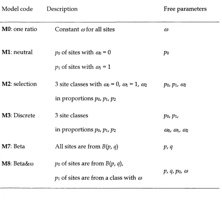
Table 1.1 - Models of œ ratio variation among sites used for simulation and

analysis

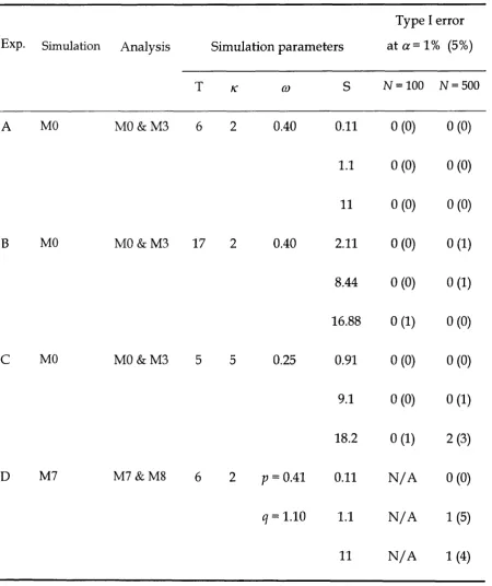
Table 2.1 - Type I error rate: number of cases out of 100 for w hich the null

hypothesis was rejected at the 1% (5%) significance levels

Table 2.2 - Power of the LRT: proportions of replicates out of 100 in which

positive selection was indicated, or detected by the LRT at the 1 %

and 5% significance levels

Table 2.3 - Comparison of the power of the standard LRT and the penalized LRT

Table 3.1 - Parameter values used in simulations

Table 3.2 - Partition of sites in a sequence used in estimation of accuracy and

power of Bayes prediction

Table 4.1 - Number of replicates (out of 100) in the likelihood analysis

comparing m odels MO (one-ratio) and M3 (discrete)

Table 4.2 - Number of replicates (out of 100) in the likelihood analysis

comparing M l (neutral) and M2 (selection)

Table 4.3 - Number of replicates (out of 100) in the likelihood analysis

comparing MO (one-tatio) and M3 (discrete)

Table 4.4 - Number of replicates (out of 100) in the likelihood analysis

comparing M7 (beta) and M8 (beta&a>)

Table 4.5 - Number of replicates (out of 100) in the likelihood analysis

comparing MO {co= 1, fixed) against MO (&> estimated)

Table 5.1 - Likelihood scores and P-values of SH test for the four inferred trees

Table 5.3 - Detecting putative recombination regions with PLATO using

HKY85 m odel with ML nucleotide frequencies and gamma rate

variation

Table 5.4 - Results of recombination tests carried out with FIST using HKY85

m odel w ith ML nucleotide frequencies and gamma rate variation

Table 5.5 - Results of LRTs and ML estimates for hepatitis delta antigen gene

Table 5.6 - Amino acids predicted to be under positive selection by Bayes

Li s t o f f i g u r e s

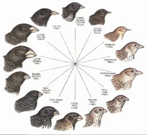
Figure 0.1. - Darwin's collection of finches

Figure 1.1 - Unrooted tree for two lineages

Figure 1.2 - An example of an unrooted 6-taxon tree used to explain likelihood

calculation and in simulation of Chapter 2

Figure 1.3 - Examples of nested models used in likelihood ratio tests for

detecting positive selection

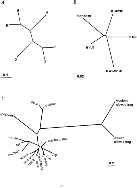
Figure 2.1 - Tree topologies used to simulate the data

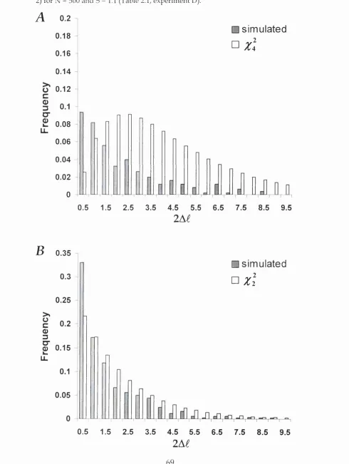
Figure 2.2. - Comparison of the distribution with the distribution of the 2A^

statistic in 500 simulated replicates

Figure 2.3. - Accuracy of the asymptotic theory for the LRT of Ho: û) = 1 against

HI: 1

Figure 3.1. - Accuracy of the Bayes prediction under M3 (discrete) for sequences

of 500 codons

Figure 3.2. - Accuracy and power of Bayes site prediction in data sets of 98

sequences

Figure 3.3 - Power of the Bayes prediction under M3 (discrete) for sequences of

500 codons

Figure 3.4 - Accuracy of the Bayesian prediction computed for one 6-taxon data

set of "infinitely" long (10^ codons) sequences using true parameter

values

Figure 3.5 - The effect of large sampling of extremely similar sequences on

accuracy and power of Bayesian prediction

Figure 3.6. - Bayes prediction of selected sites using different models.

Figure 4.1 - Accuracy of Bayes prediction of amino acid sites under positive

Figure 5.1 - Three RNAs detected in infected by HDV cells

Figure 5.2. - Phylogenies of 33 HDAg-S strains used to test data for positive

selection

Figure 5.3. - Posterior probabilities for sites in HDAg-S to evolve under positive

or purifying selection or under relaxed functional constraints in

discrete m odel M3

Figure 5.4. - Domains within hepatitis delta antigen gene

..if variations useful to any organic being ever do occur, assuredly individuals thus

characterized w ill have the best chance o f being preserved in the struggle for life; and

from the strong principle o f inheritance, these w ill tend to produce offspring sim ilarly

characterized. This principle o f preservation, or the su rvival o f the fittest, I have called

N atural Selection.

Charles Darwin, "The Origin of Species" (1859)

. ..when its whole significance dawns on you, you r heart sinks into a heap o f sand

within you. There is a hideous fatalism about it, a gh astly and damnable reduction o f

beauty and intelligence, o f strength and purpose, o f honor and aspiration.

G. Bernard Shaw on natural selection.

Ac k n o w l e d g e m e n t s a n d a u t h o r s h i p d e c l a r a t i o n

I would like to thank my supervisor Ziheng Yang (Z. Y.) for his patience, flexibility and

useful advice. I am also extremely grateful to Joseph P. Bielawski (J. B.) for many fruitful

discussions, the inspiration and moral support. It is thanks to these peoples' guidance,

advice and support the simulation studies presented in Chapters 2 - 4 resulted in the

following publications:

Anisimova, M., /. P. Bielawski, and Z. Yang. 2001. Accuracy and power of the likelihood ratio test

to detect adaptive molecular evolution. Mol. Biol. Evol. 18:1585-1592.

Anisimova, M., /. P. Bielawski, and Z. Yang. 2002. Accuracy and power of Bayes prediction of

amino acid sites under positive selection. Mol. Biol. Evol. 19:950-958.

Anisimova, M., R. Nielsen, and Z. Yang. 2003. Effect of recombination on the accuracy of the

likelihood method for detecting positive selection at amino acid sites. Genetics.164:1229-1236.

The methods overview presented in Chapter 1 and the empirical study presented

in Chapter 5 have been done solely by the author of this thesis. It was Z. Y.'s initiative to

examine the accuracy and power of methods developed by Z. Y. and collaborators. This

became the aim of my simulations, which I designed, analyzed and summarized myself.

The results presented in Chapters 2 and 3 were discussed with J. B. and Z. Y. in order to

find the best possible interpretation and draw up guidelines that would be useful for

experimental biologists using these methods. Z. Y. and J. B. helped me to develop and

improve my skills of writing a scientific report by suggesting changes (structural or

editorial) to my drafts. Work presented in Chapter 4 was initiated by the author of this

thesis. Rasmus Nielsen wrote a program to simulate recombinant data and together with

Z. Y. contributed to the discussion of Chapter 4. Z.Y. also made some suggestions and

editorial changes to parts of Chapter 4.

This work of three years would have not been possible without the financial

support from the Medical Research Council. I would also like to acknowledge Wa Yang

for discussions on viral data and for strong companionship. Robin Callard has been

helpful on many accounts. Finally, my special appreciation goes to my daughter Kristina

for love and understanding.

I

For many thousands of years a belief that species, in their present forms, were

created by God or that it was possible for organic matter to be spawned from

inorganic matter, predominated peoples' idea about the surrounding world.

But, as always, there were the skeptics w ho needed scientific explanation of the

amazing diversity of living creatures they observed around them. Early

evolutionary theories appeared during the classical Greek period w hen

Anaximander (ca. 611 - 546 BC) suggested that humans arose from fish, and,

later, Empedocles (ca. 492 - 432 BC) proposed that presently living creatures

evolved by chance combinations of elements and natural selection that led to

the extinction of once-living "monstrous" organisms. Nevertheless, western

philosophy was mostly influenced by the theories of Plato (347 - 427 BC) and

Aristotle (384 - 322 BC) w ho opposed the idea of evolution, and the

creationist-essentialist dogma that species were permanent and created for a specific

purpose became deeply embedded in western thought.

The first serious attempt to explain the species diversity in terms of

evolution was the theory of inheritance of acquired characteristics proposed in

1809 by Jean-Baptiste Lamarck (1744 - 1829). He pictured evolution as a

successive transformation of living forms from the very simple to more and

more sophisticated. His theory rested on two key mechanisms w hich pushed

species up this "great escalator of being": use and disuse - the loss of futile

inheritance of traits acquired by ancestors in response to changing

environment. For example, according to Lamarck the stretching by giraffes to

reach distant leaves led to the elongation of their necks and, hence, to offspring

with longer necks. This theory, however, was scientifically unfounded, and

gained little support in the scientific community.

A new chapter in the study of evolution was opened during the voyage

of HMS Beagle (1831 1836), with a young naturalist Charles Darwin (1809

-1882) on board. While observing animals and plants that inhabited Galapagos

Islands, Darwin noticed how animals, such as tortoise, mockingbird, and finch.

5-unr l-tNCM C4CTLÂ

H'fch

ISLAND PNOM LAAGE

CACTUS

P.KOH

rxt

ONCH PWCf-'

SMALL

k’WALL lAEfe RHCH

TFL:I=

Figure 0.1. — Darwin s collection of finches: A m ong the m ost significant specim ens

collected by Darwin during his voyage on HMS Beagle w ere 14 finch species from Galapagos

Islands, w h ich developed different habits and diets d ependent on local environm ent.

Adapted from Grant (1986).

differed from island to island morphologically. His famous collection of finches

show ed that on different islands the birds developed different eating habits,

and appropriate beak, size, and scheme of organization (Figure 0.1). These

adaptations to the different environments of the islands became important

evidence used by Darwin to formulate his theory of evolution by natural

selection proposed in Origin of Species in 1859. Darwin described evolution as

a descent with modification. Species of common ancestry adapt to fit their

individual surroundings. The natural variance within a species allows some

animals to live while others die off. As the survivors breed, they pass on the

trait that allows them to live until that trait becomes a standard feature of the

new species.

Almost sim ultaneously Alfred Wallace (1823 - 1913) independently

came to amazingly similar conclusions through his ow n work on natural

selection. Throughout the second half of the nineteenth century, Darwin and

Wallace were engaged in correspondence over the evolutionary process. The

theory of common descent and evolution by natural selection sparked an

intense debate among the fellow-scientists and underwent many modifications.

Darwin's theory seem ed to be at odds with Mendelian genetics as it did not

offer a plausible explanation of heredity. After the rediscovery of MendeTs

laws, variation in populations was shown to be caused by mutation. In 1918

R.A. Fisher for the first time described the statistical m odel of quantitative

inheritance. During the 1920s and 1930s, R.A. Fisher J.B.S. Haldane and S.

Wright pioneered the developm ent of the fundamental principles of

Darwinism and M endelism were reconciled into a new theory, known as

neo-Darwinism or synthetic theory, where mutation was recognized as the ultimate

source of genetic variation, and natural selection was thought to be dominant

in shaping the genetic makeup. The discovery of the D N A structure in 1953

revealed the molecule carrying hereditary information, marking the beginning

of new era in biological research. With the advances in molecular techniques,

more and more empirical molecular data were generated and used to examine

the genetical theory; moreover, the search for evidence of adaptation and study

of adaptive mechanisms could be done at the molecular level where the species

barrier w as no longer an issue.

H aving analyzed mammalian protein sequences, Kimura (1968a) argued

that genom ic nucleotide substitution rate was too high to be compatible with

Haldane's (1957) cost of natural selection. Subsequently, the neutral theory of

molecular evolution, independently proposed by Kimura (1968b) and by King

and Jukes(1969), challenged the Darwinian concept of natural selection stating

that the main cause of the evolutionary change and variability at the molecular

level w as random fixation of selectively neutral or nearly neutral mutations,

and that the effect of natural selection was insignificant. Neutral theory had a

progressive influence on the current state of molecular evolution: it suggested

that molecular data evolved according to stochastic rather than deterministic

processes, and provided evolutionary biologists with afalsifiable null

hypothesis. Today many aspects of the neutralist school are accepted, and the

majority of scientists agree that both weak deleterious selection and occasional

positive selection are important evolutionary factors. Adaptation could no

longer be just assumed but had to be rigorously justified. Detecting selection in

the genome became an efficient strategy for finding causes of species- specific

differences or identifying genomic regions of functional, and potentially,

medical significance. This triggered the developm ent of statistical methods that

could detect various kinds of selection and hence could identify genomic

regions of functional importance. For nucleotide data, Tajima's D-test (Tajima,

1989) became one of the m ost popular tests. Tajima's D statistic is calculated as

a scaled difference between the estimates of 4N// (where N is the effective

population size, and jj, is the mutation rate per generation) based on the

number of pairwise differences and the number of segregating sites in a sample

of sequences. Under neutrality Tajima's D is expected to be 0, whereas D < 0

and D > 0 may indicate selective sw eep and balancing selection respectively.

Several other neutrality tests, based on slightly different summary statistics,

use a similar idea (e.g.. Fay and Wu, 2000; Fu and Li, 1993). Another popular

test for nucleotide data is Hudson-K reitm an-A guade or HKA test (Hudson et

al., 1987), which evaluates the neutral hypothesis through the comparison of

variability within and between species for two or more loci. Unless the locus is

under selection, levels of polymorphism (variability within species) and

divergence (variability between species) should be proportional to the

mutation rate and, thus, should show a constant ratio of polymorphism to

divergence. Tests of selective neutrality based solely on simple summary

statistics appear powerful enough to reject the strictly neutral m odel, but such

tests are very sensitive to the demographic assumptions, making it difficult to

Simonsen, 1998). The McDonald-Kreitman or MK test (McDonald and

Kreitman, 1991) for protein coding data has been more successful at detecting

selection. The basic idea behind MK test is similar to that underlying HKA test.

The MK test compares the ratio of nonsynonym ous (amino-acid altering) to

synonym ous (silent) substitutions within and between species, w hich should

be the same in absence of selection. This test is quite robust to demographic

assumptions since the effect of the demographic m odel is the same for both

nonsynonym ous and synonym ous sites (Nielsen, 2001). H owever, HK test does

not distinguish between different forms of natural selection, and thus cannot

provide explicit evidence for adaptive evolution (Nielsen, 2001; Yang and

Bielawski, 2000). Various modifications of HK test, such as those proposed by

Akashi (1995), Templeton (1996), or Akashi (1999) provide more information

about the nature of selective forces. In particular, Akashi (1999) suggested a

way to differentiate between the types of selection by examining the frequency

distribution of observed synonym ous and nonsynonym ous changes as

compared with neutral expectation. However, w hen selection is weak, or when

the fraction of adaptive mutations is small, this method becomes considerably

less powerful. Furthermore, tests based on the idea of between and within

species comparisons require population data as w ell as species sampling. This

is not always feasible in macro-evolutionary studies.

While the relative significance of deleterious, neutral and adaptive

changes remains an open issue, detecting positive Darwinian selection became

a critical aspect of understanding the mechanisms of molecular evolution.

Adaptive evolution was show n to be responsible for changes in enzymatic

functions (Irwin, 1995; Irwin and Wilson, 1990; Stewart et al., 1987), host and

parasite co-evolution (Bishop et al., 2000; Locksley, 1997; Xiao et aL, 2002),

maintenance of the specificity of reproductive proteins (Galindo et ai., 2003;

Hellberg et al., 2000; Lee et al., 1995; Swanson et al., 2001), i.e., reproductive

isolation and thus spéciation.

The m ost rigorous way of detecting positive selection in protein coding

sequences is to show that the number of nonsynonym ous substitutions per

nonsynonym ous site is significantly higher than the number of the

synonym ous substitutions per synonym ous site. Up to now , this approach

helped to obtain the m ost convincing evidence of adaptive molecular

evolution. Chapter 1 of this thesis presents the overview of statistical methods

based on the comparison of nonsynonym ous and synonym ous rates and their

successful application to real data analysis. A special em phasis is made on the

maximum likelihood based m odels that allow a variation of the selective

pressures among sites in the protein sequence. In Chapter 2 computer

simulations are used to examine the accuracy and power of the likelihood ratio

tests (LRTs) in detecting adaptive molecular evolution. These LRTs compare

nested models of variable selective pressures among sites that were described

in Chapter 1. The empirical Bayesian approach to predict amino acids under

positive selection is introduced in Chapter 3 and subsequently evaluated by

computer simulations. Methods evaluated in Chapters 2 and 3 are

phylogeny-based and do not account for the effects of recombination. Chapter 4 therefore

presents computer simulations examining the effects of recombination on the

molecular evolution. Such thorough testing of the likelihood and Bayesian

approaches helps to evaluate the feasibility of their application to data sets of

various size and divergence. Chapter 5 presents a case study where examined

m ethods were used to detect positively selected amino acid sites. I examine a

data set of the hepatitis D antigen gene that is characterized by a large sample

and sufficient divergence, ensuring the desired accuracy and a good power of

the methods.

Chapter 1

S

M

D

P

1 .1 Me a s u r e o f t h e p o s i t i v e s e l e c t i o n p r e s s u r e o n a p r o t e i n

Adaptation has long been a subject of intense interest among evolutionary

molecular biologists. The most direct w ay of obtaining the evidence for

adaptive molecular evolution on a protein-coding gene is by identifying

amino acid sites where the nonsynonym ous (or replacement) substitution rate

dN exceeds the synonym ous (or silent) rate ds (first suggested by Miyata et al.,

1979; Miyata and Yasunaga, 1980). These rates are defined as numbers of

nonsynonym ous or synonym ous substitutions per nonsynonym ous or

synonym ous site respectively. Selective pressure at the protein level is

typically measured by the ratio co= d u / ds. If amino acid changes are

deleterious, purifying selection reduces their fixation rate, so that dw < ds and

6Ü < 1. If selection on the protein has no effect on fitness, nonsynonym ous

substitutions occur at the same rate as synonym ous substitutions and c o = l ,

suggesting neutral evolution. Only w hen amino acid changes offer a selective

advantage are nonsynonym ous changes fixed at a higher rate than

synonym ous changes. Thus a significantly higher nonsynonym ous

substitution rate, i.e. > 1, provides an evidence of adaptive molecular

evolution. Using this criterion, H ughes and Nei (1988) obtained unambiguous

evidence for positive selection in the major histocompatibility complex. Other

early studies utilized the same criterion and reported the evidence for positive

selection, for example, in variable-region genes of im m unoglobulins (Tanaka

and Nei, 1989); in gene regions encoding for T-cell epitopes in malaria

parasites (Hughes, 1991); in hemagglutinin gene of human influenza A (Ina

and Gojobori, 1994); in abalone sperm lysine (Lee et al., 1995); and the porB

gene of gonnococcus and meningococcus (Smith et al., 1995).

1 .2 E s t i m a t i o n o f a v e r a g e s y n o n y m o u s a n d n o n s y n o n y m o u s

S U B ST IT U T IO N RATES

1.2.1

Approximate methods

This section offers a brief overview of so-called ""approximate" m ethods for

estimating dw and ds rates. All such methods approximate rates dw and ds

using intuitive assum ptions rather than rigorous theory. Although they

greatly differ in detail, the basic procedure is the same: (i) count the numbers

of synonym ous and nonsynonym ous sites in the observed sequences; (ii)

count the numbers of synonym ous and nonsynonym ous differences by

considering all possible evolutionary pathways between the hom ologous

codons; (iii) correct for multiple substitutions at the same sites using a

standard evolutionary model.

Miyata and Yasunaga (1980) proposed one of the first m ethods for

estimating synonym ous and nonsynonym ous rates. Its simplified version (Nei

and Gojobori, 1986) gave essentially the same estimates of Jn and ds, and

subsequently became very popular. Considering the likelihood of a nucleotide to

result in a silent or replacement substitution in each of the three codon positions,

Nei-Gojobori method computes total numbers of synonym ous (S) and

comparisons the averages of S and N for the two sequences are used. The total

numbers of synonym ous (Sd) and nonsynonym ous (Nd) pairwise differences are

counted, again, by adding respective counts for all codons. When there is more

than one difference between the hom ologous codons, all possible evolutionary

pathways are considered and w eighted equally. The proportions of synonym ous

(ps) and nonsynonym ous (pw) differences can be approximated by the equations:

ps = Sd/ S and pN = Nd / N. Synonymous and nonsynonym ous rates are estimated

using Jukes and Cantor(1969) formula as a correction for multiple substitutions:

ds = - % lo g (l - 4/3ps) and dN = - % log(l - 4/3p^). Both Miyata-Yasunaga and

Nei-Gojobori methods are based on Jukes and Cantor nucleotide substitution

m odel (JC69), assume equal nucleotide frequencies, and ignore the

transition/ transversion bias. The latter is known to cause underestimation of the

number of synonym ous sites and overestimation of nonsynonym ous sites since

at the third codon positions transitions are more likely to be synonym ous than

are transversions. The problem becomes especially serious w hen sequences are

highly diverged.

Li et al. (1985) extended Miyata-Yasunaga method so 2-fold, 4-fold, and

non-degenerate nucleotide sites were treated separately (as in Perler et al., 1980),

using Kimura's (1980) 2-parameter model to correct for multiple hits. However,

JC69 m odel was still used as an underlying mutation matrix. After numerous

attempts to account for transition/ transversion rate bias (Comeron, 1995; Li,

1993; Pamilo and Bianchi, 1993) in all steps of the estimation this has been

achieved by Ina (1995) in his unweighted pathway method based on Kimura's

parameter model. Ina's (1995) simulations show ed that m ethods of

Miyata-Yasunaga, Nei-Gojobori and Li et al. caused underestimation of dN and

overestimation of ds by overestimating N and underestimating S. According to

the same study, the method of Pamilo and Bianchi and Ina's new method give

better estimates of dhi and ds) but for data with strong transition/ transversion

and nucleotide frequency biases all the above-mentioned m ethods give biased

estimates as none of them account for unequal base composition. Similar

concerns have been expressed in other studies (Bielawski et al., 2000; Moriyama

and Powell, 1997; Yang and Nielsen, 2000). Interestingly, the effect of nucleotide

bias can override the effect of transition/transversion bias. For example, in

studies of mammalian nuclear genes (Ohta, 1995; Yang and Nielsen, 1998) biased

codon frequencies led to reduced numbers of synonym ous sites; as a result,

contrary to the general belief, Nei-Gojobori method overestimated rather than

underestimated S and co.

Finally, Yang and Nielsen (2000) incorporated transition/transversion

bias and unequal base frequencies in every step of their iterative algorithm

assuming the HKY85 nucleotide substitution m odel (Hasegawa et al., 1985).

Estimates of dN and ds produced by this new approximate m ethod were

shown to be very close to the true values even for data with strong

1.2.2 Maximum likelihood estimation of positive selection pressure

The concepts of likelihood and maximum likelihood estimation

Maximum likelihood (ML) is a major statistical inference tool, w hich is widely

used in a variety of fields. The idea central to this method is to choose a

hypothesis that maximizes the likelihood of the observed data (i.e., makes the

data the m ost plausible). ML inference is based on an explicit probabilistic

model, and a hypothesis is defined as a certain set of the parameters

describing that model. Although in some cases the ML approach can be

computationally intensive, the advantages of em ploying it are apparent: (i)

ML is a classical statistical technique, it is w ell studied and has useful

statistical properties; (ii) parameters of interest can be estimated by

maximizing the likelihood of observing the data; (iii) ML enables formulation

of a variety of hypotheses as w ell as testing those hypotheses by likelihood

ratio tests (LRTs), (iv) ML can be used as a framework for Bayesian inference,

the benefits of which are predicting the most probable scenarios and

quantifying the uncertainty of such predictions in an easily interpretable

form.

More formally, if a probabilistic model is formulated in terms of

unknown parameters 6 = {Qi, ... ^»), the likelihood of the hypothesis

described by 9 is proportional to the probability of the observed data given that

hypothesis is correct. Thus, a likelihood function is defined as a joint

probability density function of all independent observations x = given

parameters 0\ l { x

|

%

%

... %

» I

=/(^i I ^/(%2 I 0 ./(%« I

unknown parameters 0 are estimated by maximising the probability of

observing data x given 6 . Let è be the ML estimator (MLE) that evaluates the

parameters 9 so it maximises the likelihood

L(% |

called an ML estimate.

As the likelihood function is a product of probabilities for all

observations it can be very close to 0. It is therefore easier to work with the

logarithm of L(% | 9). Let ^{9) = log L{9). The log-likelihood function is

maximised by solving £'(9) = 0 and t ' { 9 ) < 0. In simple cases it is possible to

solve the equation analytically. However, in the majority of cases this is done

using numerical procedures such as repeated bisection or Newton-Raphson

method.

The attraction of using ML for parameter estimation lies in the

following properties offered by the MLE 0 for regular cases (e.g., Stuart et al.,

1999; Wald, 1949):

(i) 0 is asymptotically unbiased, meaning that for large enough samples its

expectation is equal to the true value: E [ 0 ] = %

(ii) 0 is asymptotically efficient, which means that for large samples the MLE is

the estimator w ith the low est possible variance;

(iii) 0 is asymptotically normally distributed around the true value 6b with a

minimum possible variance;

(iv) 6 is a consistent estimator of 9. as the sample size increases 0 converges to

(v) à is transformation-invariant: if a single-valued twice-differentiable function

g(0) has g ' ( 0 ) ^ 0 for any 6, then g ( 0 ) is an ML estimator of

Maximum likelihood and Bayesian methods are now successfully used in

phylogenetics (Lewis, 2001; Whelan et al., 2001). The use of the ML approach in

molecular phylogenetics was first suggested by Cavalli-Sforza and Edwards

(1967). H owever, the computationally effective algorithm for calculating a

likelihood of a phylogeny was first presented by Felsenstein (1973,1981). The

ML framework, originally developed for continuous characters (Felsenstein,

1973), was later adapted to accommodate nucleotide (Felsenstein, 1981), amino

acid (Adachi and Hasegawa, 1992; Kishino et al., 1990) and codon data

(Goldman and Yang, 1994; Muse and Gaut, 1994). Since this thesis focuses on

ML m odels for coding data, the next section is devoted to stochastic models of

coding sequence evolution.

Markov codon models

Explicit probabilistic m odels of codon substitution on a phylogeny were

proposed by Goldman and Yang (1994) and Muse and Gaut (1994). These

studies demonstrated that ML was flexible in respect to a variety of

parameters that could be incorporated to reflect the transition/transversion,

codon usage biases, synonym ous and nonsynonym ous rates, and other

particulars such as chemical differences between amino acids. The m odel of

Muse and Gaut incorporated only variable nucleotide frequencies and

separate synonym ous and nonsynonym ous rates. Although incorporating

transition/transversion rate and accounting for variable codon (or amino

acid) frequencies w ould have been more realistic. Muse and Gaut (1994)

admitted this but chose a simple scenario demonstrating the technique with

minimal parameters incorporated. Goldman and Yang (1994) presented a

more realistic model, which accounted for non-uniform codon frequencies,

transition/ transversion bias and incorporated a separate parameter to

measure the gene variability. The latter parameter implicitly represented the

tendency of the gene to undergo nonsynonym ous substitutions, and was

positively correlated with the 6) ratio. In an attempt to account for selective

differences at the amino acid level Goldman and Yang (1994) used

Grantham's (1974) matrix of physiochemical distances. H ow ever, Grantham's

m odel of protein evolution was fully based on physicochemical properties

and could not directly reflect the amino acid differences enforced by

evolution. Subsequently, the m odel of Goldman and Yang (1994) w as

simplified to incorporate the 6? ratio explicitly (e.g., N ielsen and Yang, 1998).

Described versions of the codon substitution m odels are the same

conceptually, but differ in their definition of the rate matrix Q. The evolution

of codons is m odelled by a continuous-time Markov process running along a

phylogeny. Suppose p,)(f) is the probability that codon i changes into codon;

over time f. Here i and j take values from 1 to 61 representing all sense

codons. The time interval t is measured by the expected number of nucleotide

substitutions per codon (often referred to as a branch length). Transition

substitution rate from codon i to codon; is described by matrix Q = [qij]. The

m ost successful matrix incorporates codon frequencies tTj,

transition/transversion rate ratio k , and nonsynonym ous/synonym ous rate

ratio œ (simplified m odel of Goldman and Yang, 1994):

0, if / and j differ at 2 or 3 nucleotide positions

71 j , if / and j differ by 1 synonymous transversion

q.j = <1 KTTj, if i and j differ by 1 synonymous transition (1)

C07t J, if i and j differ by 1 nonsynonymous transversion

coKTTj, if i and j differ by 1 nonsynonymous transition

Substitutions are assumed to occur independently am ong the three codon

positions: only one position is allowed to change instantaneously. Note also

that diagonal values are calculated so the rows sum up to 0: qu= - ^ for

i*j

any i (e.g., Grimmet and Stirzaker, 1992, p. 241). Since time and rate of change

are confounded, the rate matrix is multiplied by a scaling factor so that the

expected number of nucleotide substitutions per codon is one:

- ^ 7T^q^. q^j = 1. All codon sites in a sequence are assum ed to evolve

i I t* j

independently according to the same Markov process (in statistical terms,

codons at different sites are independently and identically distributed).

The rate of change of the transition probability is d P { t ) / d t = P (t)x Q .

The solution of this equation with the initial conditions d P { 0 ) / d t = I (where I

is the identity matrix) is an exponential P(t)=eQ^. This can be calculated using

Taylor expansion: F(t) = ^ (Qf)”/ ^1/ where the number of terms in Taylor

n=Q

expansion is determined by a desired accuracy level. Another w ay of

calculating P{t) is through diagonalization (or spectral decomposition) of Q:

P (t) = U x diag{g^'' } x U ~ \ where U is the matrix containing eigenvectors

of Q and À i , À n are the eigenvalues of Q.

The Markov process defined by equation (1) is time reversible, i.e., in

any time t, the amount of change from codon z to j is assum ed to be the same

as the amount of change from codon; to codon z, and so mpij(t) =7Tjpji(t). This

property is convenient mathematically, and although it m ight not be justified

biologically, it is commonly assumed since the direction of codon change in

the observed data is unknown. Note also that the rate matrix is independent

of time meaning that the process of codon substitution is assumed to be the

same in different parts of the tree. This property is referred to as homogeneity;

the equilibrium distribution of a homogeneous process is also a limiting

distribution w hen time approaches infinity. Moreover, the process of codon

substitution is typically assumed to be stationary, im plying that the

evolutionary process remains at the equilibrium throughout time, i.e., codon

frequencies are approximately the same during the w hole course of the

evolution. Both hom ogeneity and stationarity are unrealistic assumptions

since the divergence rates, nucleotide composition (or other biases) may differ

in time, especially for distantly related lineages (e.g., Yang and Roberts, 1995;

Rodriguez-Trelies et al., 2001). To correct for this, non-hom ogeneous

Markov-process m odels were proposed (Yang and Roberts, 1995; Galtier and Gouy,

1998; also see Section 1.4). These models allow for different patterns of

hom ogeneity and stationarity are made for the convenience of computation,

rather than to reflect the biological reality.

ML estimation of the

ratio for two sequences and its accuracy

Once a probabilistic m odel is formulated, the likelihood function of the parameters is

constructed and maximized. Let the data contain two aligned protein-coding

sequences (Figure. 1.1), with the alignment length of N codons (sites). Then the

61

probability of observing data Xh = {i , j ) at codon site h is L(xh) = '

X r=1

where xr is the state at the root of the tree, and h and h are the lengths of the

branches connecting the root with sequences at the tips. However, the location of the

root is unknown and time-reversibility of the m odels implies that the same

probability can be calculated w hen one of the sequences is assum ed to be ancestral

to another: L(xh) = TUjPjj (f^+y or L(xh) (^1+^2)- The result remains the same

irrespective of the sequence assumed to be ancestral. That means the root of the tree

is unidentifiable, so only the sum t = h + can be estimated, but not h and ti

separately. The log-likelihood function for the w hole alignment is: k , co, )) =

N

^log{;r,p^ (r)}. Codon frequencies m are usually estimated using the observed base

h = \

Seq.l

Seq.2

Figure 1.1. - Unrooted tree for two lineages:

d u e to the reversible nature o f co d o n m od els, the

location o f root R is u n k n o w n , so on ly su m of

branch len gth s ti + tz can be estim ated.

frequencies at the three codon positions. Parameters t, k , and œ are estimated by

m axim izing the log-likelihood function. Rates dw and d s are calculated as functions

o f ML estimates of t, k , and co. By property (5) stated on p. 20, estimates of dw and d s

are also ML estimates, and therefore bear the same properties (see p. 20). In more

detail (e.g., Goldman and Yang, 1994), the proportions of synonym ous and

nonsynonym ous substitutions per codon are defined as p i = ^ Tr^qy and

'V

= \ - pI , respectively. The summation is taken for all distinct codons i and j

representing the same amino acid aui = auj. The numbers of synonym ous and

nonsynonym ous substitutions per codon are tp l and /p^, respectively. Next, the

proportions of synonym ous and nonsynonym ous sites, p \ and p \, are calculated as

pI and pI but assum ing c o = l , i.e., no natural selection at the protein level. The

numbers of synonym ous and nonsynonym ous sites per codon are respectively

?>pI and 3pjy. Synonymous and nonsynonym ous rates per site can be now calculated

as follows: = tpH{?>pl) and = % /(3 p ]^ ).

Bielawski et al. (2000) evaluated the impact of the estimation method

for 82 mammalian nuclear genes. They have demonstrated that failure of the

approximate m ethods of Nei-Gojobori (1986) and Ina (1995) to properly

account for transition/ transvertion rate bias and unequal codon usage led to

misleading conclusions about patterns of mammalian nuclear gene evolution.

Simulation study of Yang and Nielsen (2000) compared four methods

for estimating and ds for two sequences: Nei-Gojobori and Ina's methods,

contrast to ML, all three approximate methods are biased and inconsistent,

w hich was confirmed by simulation (Yang and Nielsen, 2000). H owever, for

infinite data in almost all scenarios method of Yang and N ielsen had the

smallest biases and gave similar estimates to those obtained by ML.

Furthermore, for finite data for almost all cases the ML m ethod w as show n to

be the least biased w ith lower mean squared error (MSB, defined as E [(é

-= var[^] + \ E { è \ - 6 Y ) compared to the approximate methods. This

suggested that ML method should be preferable over the ad hoc

approximations. Additionally, the probability theory underlying the ML

approach makes the method conceptually more comprehensive and flexible to

account for a variety of factors. ML accounts for all possible pathways of

codon substitution and weights them according to relative probabilities of

their occurrence; and at the same time ML naturally resolves the task of

correcting for multiple hits, which is otherwise very difficult. Finally, the ML

framework can easily accommodate comparison of multiple sequences taking

into account their phylogenetic relationship, - an advantage approximate

m ethods lack.

1 .3 M e t h o d s a l l o w i n g v a r i a t i o n o f s e l e c t i v e p r e s s u r e a m o n g s i t e s

Methods assuming the same a> ratio for all sites only detect positive selection

if the average co> 1 (Yang and Bielawski, 2000). Just a few years ago, cases of

positive selection have been difficult to demonstrate. A large-scale database

search performed by Endo et al. (1996) identified only 17 out of 3,595 genes

that might have undergone adaptive evolution. Endo et al. (1996) considered

a gene to be under positive selection if the average dw w as greater than ds in

more than half of the pairwise sequence comparisons. This approach

computes the co ratio as an average across all amino acid sites and over time;

although popular, it has little power. For example, Crandall et al. (1999) found

that the approach of pairwise comparison failed to detect positive selection in

the protease gene of HIV-1 despite clear evidence of parallel evolution.

Crandall et al. (1999) suggested that the ty ratio averaged over sites was a poor

indicator of positive selection. Indeed, the assumption that all sites in a

sequence are under equal selective pressure is unrealistic. Typically adaptive

evolution occurs at only a few sites as most amino acids in a protein are under

structural and functional constraints with dw and, hence co, close to 0 (e.g.,

Golding and Dean, 1998). Moreover, those few sites m ight not be clustered in

a sequence, since sites that are far apart in a primary sequence can be

clustered in the three-dimensional structure. Thus calculating co as an average

over all amino acid sites substantially reduces the power to detect positive

selection, and even sliding w indow analysis m ight not detect positive

Darwinian selection in many genes (e.g., Endo et al., 1996).

Much effort has been taken to account for variable selective pressures

across sites to improve the power of the methods for detecting positive

selection. Most of such methods do not take a priori know ledge about the kind

of selective pressure acting on particular sites (e.g.. Bush et al., 1999; Fitch et

Yamaguchi-Kabata and Gojobori, 2000; Yang et al., 2000a). In a classical study of the MHC

class I (Hughes and Nei, 1988) all amino acid residues were partitioned into

those that belong to the antigen-recognition region and those that are outside.

The evidence of positive selection was obtained by comparing and ds rates

in each partition. Yang and Swanson (2002) implem ented an ML method for

pre-partitioned data sets and applied it to the human MHC class I and

abalone sperm lysin genes previously analyzed by H ughes and N ei (1988)

and Lee et al. (1995) respectively. To account for heterogeneity among the site

partitions, they used a separate œ ratio for each partition.

Note that all m ethods mentioned above assume a constant fy ratio for

all lineages, and thus have low power of detecting positive episodic or

directional selection but have been successful in detecting recurrent

diversifying selection.

1.3.1

Methods based on ancestral reconstruction

Most non-likelihood methods that account for variable selective pressures

reconstruct sequences of the extinct ancestors; then, at each site, count

changes along the tree to identify sites with an excess of nonsynonym ous

substitutions. Fitch et al. (1997) analysed 254 sequences of the hemagglutinin

(HA) gene of human influenza A and found possible sites under positive

selection. They used parsimony ancestral reconstruction and tested whether

the proportions of nonsynonym ous and synonym ous substitutions at each

sites deviated from binomial expectations calculated using the total numbers

of non-synonym ous and synonym ous substitutions. Effectively, this meant

that the comparison was made with averages over all sites, w hich is not a

stringent enough criterion as the average of the co ratio over all sites in a gene

is usually < 1. Thus, this method might have high false positive rate. Later,

Bush et al. (1999) examined a larger hemagglutinin data set using a slightly

modified m ethod of Fitch et al. (1997). The authors attempted to correct for

uncertainties introduced by variation in the tree topology, and used a more

stringent criterion whereby expected substitution rates were calculated across

sites excluding the codons with a significant excess of nonsynonym ous

substitutions over synonym ous. A more systematic approach w as developed

by Suzuki and Gojobori (1999). They estimated numbers of synonym ous and

nonsynonym ous sites and the substitutions using ancestral sequences

reconstructed by parsimony and tested whether there w as a significant

deviation from the neutral expectation ” ( o = l " . Data sets of human HLA, V3

region of HIVI env gene, and the H A gene of human influenza A were

examined for positive selection. At least 200 sequences were used in each

analysis. N ote, only 3 codons were suggested to be under positive selection in

influenza H A gene; that is in contrast to 25 codons suggested by the method

of Fitch et al. (1997). A method conceptually very similar to that of

Suzuki-Gojobori m ethod was applied to analyze 186 sequences from HIV l gpl20

(Yamaguchi-Cabata and Gojobori, 2000).

Naturally, all the above m ethods require large samples so there are

reconstruction can reduce the accuracy of the results produced by these

methods. For divergent samples of sequences, the parsimonious ancestral

reconstruction is highly unreliable, rendering analyses of such data

unfeasible. Moreover, parsimony considers only the reconstructions with a

m inimum amount of changes and so can seriously underestimate the total

number of changes (as shown by Nielsen, 2002). N ot only can the

parsimonious solution be unlikely but there could be non-parsimonious

reconstructions that are much more likely (Nieslen, 2002). Furthermore, the

above m ethods cannot easily account for molecular biases, for example in

data sets with high transition/ transversion ratio bias the numbers of

transitions w ould be underestimated. Finally, none of the above-mentioned

m ethods offer a mathematically rigorous solution to measuring the

confidence in sites inferred to be under positive selection.

Recently N ielsen and Huelsenbeck (2002) proposed a statistically

rigorous alternative that avoids problems associated w ith using parsimony

and relying on a single reconstruction. Referring to a reconstruction as a

mapping of mutations on a phylogeny, the authors formulate numbers of

nonsynonym ous and synonym ous changes as functions of the mapping, so

they can be inferred for any mapping directly. Since the correct m apping is

unknown, the authors suggest computing the conditional (on data)

expectation of nonsynonym ous and synonym ous changes by which all

mapping possibilities are considered and weighted accordingly. This requires

calculating a posterior probability of a mapping, which is evaluated in

Bayesian framework. While the ML method requires a phylogeny to be

known, the method of Nielsen and Huelsenbeck (2002) takes it as one of the

nuisance parameters which is integrated out via Markov chain Monte Carlo

(MCMC) technique. The current implementation assumes general

time-reversible nucleotide m odel and uniform parameter priors. H owever, using a

codon m odel of evolution w ould be more appropriate for incorporating

differences in rates of nonsynonym ous and synonym ous substitutions.

Hypotheses are tested by comparing the posterior and posterior predictive

(expected) distributions of the statistics of interest using posterior predictive

P-values (Meng, 1994). This new method was applied to the 28 sequences of

the H A gene from human influenza A. The same data set w as previously

analyzed by Yang et al. (2000a) and is a subset of sequences originally

analyzed by Fitch et al. (1999). Remarkably, Nielsen and Huelsenbeck (2002)

detected sites under positive selection that were essentially the same as those

identified by the ML method (Yang et al., 2000a). The method of posterior

predictive P-values can be easily extended and adapted to address a variety of

problems but its statistical properties ought to be studied further. This is out

of the scope of the study presented here, and I w ill be focusing on evaluating

the performance of ML m ethods that account for variable selective pressure

across the sequence (Nielsen and Yang, 1998; Yang et al., 2000a). These

methods are described in detail in the next section (Section 1.3.2). Note, ML

approach does not rely on the ancestral reconstruction and so does not suffer

calculated for each site provide an intuitive measure of the confidence in a

prediction.

1.3.2 Models implemented within maximum likelihood framework

Nielsen and Yang (1998) and Yang et al. (2000a) developed codon-based

models that account for variation of the co ratio among sites. In these models

the CO ratio takes values from a number of discrete site classes or from a

continuous distribution. ML models of among site co-variation are

implemented in the ML framework and can be used: (i) to test for presence of

codon sites affected by positive selection, and (ii) to identify such sites when

they exist using Bayesian inference. Although ML m odels can be

computationally intense for large number of lineages, they do not rely on

ancestral reconstruction like methods described in the previous section, and

so can tolerate divergent data.

The ML approach involves the likelihood ratio test (LRT) of two nested

models, one of which does not account for sites with cy > 1 w hile another

does. A gene is considered to be under positive selection if (i) the LRT is

significant, and (ii) at least one of the ML estimates of cy is > 1. When the ML

parameter estimates and the LRT indicate presence of sites under positive

selection, the empirical Bayesian approach can be used to predict them

(Nielsen and Yang, 1998; Yang et al., 2000a). One com putes the posterior

probability that a site belongs to each co class of the m odel given the data at