Diego F. Aranha1, Pierre-Alain Fouque2, Chen Qian3, Mehdi Tibouchi4, and Jean-Christophe Zapalowicz5
1
Institute of Computing, University of Campinas,[email protected]
2
Universit´e de Rennes 1 and Institut Universitaire de France,[email protected]
3 ENS Rennes,[email protected] 4
NTT Secure Platform Laboratories,[email protected]
5 Inria,[email protected]
Abstract. Applications of elliptic curve cryptography to anonymity, privacy and censorship circumvention call for methods to represent uniformly random points on elliptic curves as uniformly random bit strings, so that, for example, ECC network traffic can masquerade as random traffic.
At ACM CCS 2013, Bernstein et al. proposed an efficient approach, called “Elligator,” to solving this problem for arbitrary elliptic curve-based cryptographic protocols, based on the use of efficiently invertible maps to elliptic curves. Unfortunately, such invertible maps are only known to exist for certain classes of curves, excluding in particular curves of prime order and curves over binary fields. A variant of this approach, “Elligator Squared,” was later proposed by Tibouchi (FC 2014) supporting not necessarily injective encodings to elliptic curves (and hence a much larger class of curves), but, although some rough efficiency estimates were provided, it was not clear how an actual implementation of that approach would perform in practice.
In this paper, we show that Elligator Squared can indeed be implemented very efficiently with a suitable choice of curve encodings. More precisely, we consider the binary curve setting (which was not discussed in Tibouchi’s paper), and implement the Elligator Squared bit string representation algorithm based on a suitably optimized version of the Shallue–van de Woestijne characteristic2encoding, which we show can be computed using only multiplications, trace and half-trace computations, and a few inversions.
On the fast binary curve of Oliveira et al. (CHES 2013), our implementation runs in an average of only 22850 Haswell cycles, making uniform bit string representations possible for a very reasonable overhead—much smaller even than Elligator on Edwards curves.
As a side contribution, we also compare implementations of Elligator and Elligator Squared on a curve supported by Elligator, namely Curve25519. We find that generating a random point and its uniform bitstring representation is around 35–40% faster with Elligator for protocols using a fixed base point (such as static ECDH), but 30–35% faster with Elligator Squared in the case of a variable base point (such as ElGamal encryption). Both are significantly slower than our binary curve implementation.
Keywords: Elligator, Binary Elliptic Curves, Efficient Implementation, PCLMULQDQ, Anonymity & Privacy.
1 Introduction
Elliptic curves offer many advantages for public-key cryptography compared to more traditional settings like RSA and finite field discrete logarithms, including higher efficiency, a much smaller key size that scales gracefully with security requirements, and a rich geometric structure that enables the construction of additional primitives like bilinear pairings. On the Internet, adoption of elliptic curve cryptography is growing in general-purpose protocols like TLS, SSH and S/MIME, as well as anonymity and privacy-enhancing tools like Tor (which favors ECDH key exchange in recent versions) and Bitcoin (which is based on ECDSA).
To alleviate that problem, one possible approach is to modify protocols so that transmitted points randomly lie either on the given elliptic curve or on its quadratic twist (and the curve parameters must therefore be chosen to be twist-secure). This is the approach taken by M¨oller [23], who constructed a CCA-secure KEM with uniformly random ciphertexts using an elliptic curve and its twist. This approach has also been used in the context of kleptography, as considered by Young and Yung [30,31], and has already been deployed in circumvention tools, including StegoTorus [28], a camouflage proxy for Tor, and Telex [29], an anticensorship technology that uses a covert channel in TLS handshakes to securely communicate with friendly proxy servers. However, since protocols and security proofs have to be adapted to work on both a curve and its twist, this approach is not particularly versatile, and it imposes additional security requirements (twist-security) on the choice of curve parameters.
A different approach, called “Elligator,” was presented at ACM CCS 2013 by Bernstein, Hamburg, Krasnova and Lange [6]. Their idea is to leverage an efficiently computable, efficiently invertible algebraic function that maps the integer intervalS={0, . . . ,(p−1)/2},pprime,injectivelyto the groupE(Fp)where
Eis an elliptic curve overFp. Bernstein et al. observe that, sinceιis injective, a uniformly random pointP
inι(S) ⊂E(Fp)has a uniformly random preimageι−1(P)inS, and use that observation to represent an
elliptic curve pointP as the bit string representation of the unique integerι−1(P)if it exists. If the primepis close to a power of2, a uniform point inι(S)will have a close to uniform bit string representation.
This method has numerous advantages over M¨oller’s twisted curve method: it is easier to adapt to existing protocols using elliptic curves, since there is no need to modify them to also deal with the quadratic twist; it avoids the need to publish a twisted curve counterpart of each public key element, hence allowing a more compact public key; and it doesn’t impose additional security requirements like twist-security. But it crucially relies on the existence of an injective encodingι, only a few examples of which are known [13,17,6], all of them for elliptic curves of non-prime order over large characteristic fields. This makes the method inapplicable to implementations based on curves of prime order or on binary fields, which rules out most standardized ECC parameters [15,11,22,1], in particular. Moreover, the rejection sampling involved (when a pointP is picked outsideι(S), the protocol has to start over) can impose a significant performance penalty.
To overcome these limitations, Tibouchi [27] recently proposed a variant of Elligator, called “Elligator Squared,” in which a pointP ∈E(Fq)is represented not by a preimage under an injective encodingι, but
by a randomly sampled preimage under an essentially surjective map F2q → E(Fq)with good statistical
properties, known as anadmissible encodingfollowing a terminology introduced by Brier et al. [10]. By results due to Farashahi et al. [14], such admissible encodings are known to exist for all isomorphism classes of elliptic curves, including curves of prime order and binary curves. Since admissible encodings are essentially surjective, the approach also eliminates the need for rejection sampling at the protocol level.
Our contributions. While the Elligator Squared approach is quite versatile, its efficiency is highly dependent on how fast the underlying admissible encoding can be computed and sampled, and the same can be said of Elligator in the settings were it can be used. Since, to the best of our knowledge, no detailed implementation results or concrete performance numbers have been published so far for the underlying encodings, one only has some rough estimates to go by. For Elligator, Bernstein et al. give ballpark Westmere cycle count figures based on earlier implementation results [7], and for Elligator Squared, Tibouchi provides some average operation counts in [27] for a few selected encoding functions. No performance-oriented implementation is available for either approach.
We propose various algorithmic improvements and computation tricks to obtain a fast evaluation of the binary Shallue–van de Woestijne encoding and of the associated Elligator Squared sampling algorithm. In particular, our description is much more efficient than the one given in [9, Appendix E].
Based on these algorithmic improvements, we performed software implementations of Elligator Squared on the record-setting binary GLS curve of Oliveira et al. , defined overF2254 [24]. We dedicate special attention
to optimizing the performance-critical operations and introduce corresponding novel techniques, namely a new point addition formula inλ-affine coordinates and a faster approach for constant-time half-trace computation over quadratic extensions ofF2m. Moreover, timings are presented for both variable-time and constant-time
field arithmetic.6The resulting timings compare very favorably to previously suggested estimates.
Finally, as a side contribution, we also propose concrete cycle counts on Ivy Bridge and Haswell for both Elligator and Elligator Squared on the Edwards curve Curve25519 [4] based on the publicly available implementation of Ed25519 [5]. We find that, on this curve, the Elligator approach is roughly 35–40% faster than Elligator Squared for protocols that rely on fixed-base scalar multiplication, such as ECDH, but conversely, for protocols that rely on variable-base scalar multiplication like ElGamal encryption, Elligator Squared is 30–35% faster. Both approaches are significantly slower than what we achieve on the same CPU with our binary curve implementation.
2 Preliminaries
LetEbe an elliptic curve over a finite fieldFq.
2.1 Well-bounded encodings
Definition 1. A functionf :Fq →E(Fq)is said to beB-well-distributed encoding for a certain constant
B >0if for any nontrivial characterχofE(Fq), the following holds:
X
u∈Fq
χ(f(u))
≤B√q.
Definition 2. We call a functionf :Fq →E(Fq)a(d, B)-well-bounded encoding, for positive constants
d, B, whenf isB-well-distributed and all points inE(Fq)have at mostdpreimages underf.
2.2 Elligator Squared
Letf :Fq→E(Fq)be a(d, B)-well-bounded encoding and letf⊗2the tensor square defined by:
f⊗2 :F2q →E(Fq)
(u, v)7→f(u) +f(v).
Tibouchi shows in [27] that if we sample a uniformly random preimage underf⊗2of a uniformly random pointP on the curve, we get a pair(u, v)∈F2q which is statistically close to uniform. Moreover he proves
that sampling uniformly random preimages under f⊗2 can be done efficiently for all pointsP ∈ E(Fq)
except possibly a negligible fraction of them [27, Theorem 1]. The sampling algorithm Tibouchi proposed is described as Algorithm1. The idea is to randomly pick a randomuand then to compute a correct candidatev such thatP =f(u) +f(v). The last steps of the algorithm (step 5 to 7) are also needed in order to ensure the uniform distribution of the output(u, v).
6
Algorithm 1Preimage sampling algorithm forf⊗2.
1: functionSAMPLEPREIMAGE(P) 2: repeat
3: u←$ Fq 4: Q←P−f(u)
5: i←#f−1(Q)
6: j← {$ 1,· · ·, d} 7: untilj≤i
8: {v1,· · ·, vt} ←f−1(Q) 9: return(u, vj)
10: end function
2.3 Shallue–van de Woestijne in Characteristic 2
In this section, we recall the Shallue–van de Woestijne algorithm in characteristic 2 [25], following the more explicit presentation given in [9, Appendix E]. An elliptic curve over a fieldF2n is a set of points
(x, y)∈(F2n)2verifying the equation:
Ea,b:Y2+X·Y =X3+a·X2+b
wherea, b ∈ (F2n)2. Letg be the rational functionx 7→ x−2·(x3+a·x2 +b).LettingZ = Y /X, the
equation forEa,bcan be rewritten asZ2+Z =g(X).
Theorem 1. Letg(x) =x−2·(x3+a·x2+b)wherea, b∈(
F2n)2. Let
X1(t, w) =
t·c
1 +t+t2 X2(t, w) =t·X1(t, w) +c X3(t, w) =
X1(t, w)·X2(t, w)
X1(t, w) +X2(t, w)
where c = a+w+w2. Then g(X1(t, w)) +g(X2(t, w)) +g(X3(t, w)) ∈ h(F2n) where his the map
h:z7→z2+z.
From Theorem 1, we have that at least one of theg(Xi(t, w)) must be inh(F2n), which leads to a
point inEa,b(F2n). Indeed, we have thath(F2n) = {z∈ F2n|Tr(z) = 0}, whereTris the trace operator
Tr :F2n →F2 with:
Tr =
n−1 X
i=0
z2i
(one inclusion is obvious and the other one follows from the fact that the kernel of theF2-linear maph
is{0,1}, hence its image is a hyperplane). As a result,P3i=1Tr(g(Xi)) = 0and therefore at least one of
theXi must satisfyTr(g(Xi)) = 0sinceTrisF2-valued. Such anXi is indeed the abscissa of a point in
Ea,b(F2n), and we can find itsy-coordinate by solving the quadratic equationZ2+Z =g(Xi). That equation
isF2-linear, so findingZamounts to solving a linear system overF2. This yields the point-encoding function
described in Algorithm2.
In the description of that algorithm, the solution of the quadratic equation is expressed in terms of the mapQS :F2n →F2n (“quadratic solver”), which is the well-defined linear map such that, for allx,QS(x)is
the trace zero solution of the quadratic equationz2+z=x+ Tr(x). Whennis odd,QSis straightforward to compute: it is the half-trace mapHTrdefined as:
HTr :z7→
(n−1)/2 X
i=0
Algorithm 2Shallue–van de Woestijne algorithm in characteristic 2. Require: a, b∈F2nandt, w∈F2n
Ensure: (x, y)∈Ea,b 1: c←a+w+w2
2: X1←t·c/(1 +t+t2) 3: X2←t·X1+c
4: X3←X1·X2/(X1+X2) 5: forj= 1to 3do
6: hj←(Xj3+a·X 2 j +b)/X
2 j
7: ifTr(hj) = 0then return(Xj,QS(hj)·Xj) 8: end if
9: end for
We discuss the efficient computation ofQSin even degree extensions in§4.
Algorithm2actually maps two parameterst, wto a rational point on the curveEa,b. One can obtain a
mapf:Fq→Ea,b(Fq)by picking one of the two parameters as a suitable constant and letting the other one
vary. In what follows, for efficiency reasons, we fixtand usewas the variable parameter.
One can check that the resulting function is well-bounded in the sense of§2.1. Indeed, the framework of Farashahi et al. [14] can be used to establish that it is a well-distributed encoding: the proof is easily adapted from the one given in [18] for the positive characteristic version of the Shallue–van de Woestijne algorithm. Moreover, each curve point has at most6preimages under the corresponding function: there are at most two values ofwthat yield a given value ofX1, and similarly forX2, X3. Thus, we obtain a(d, B)-well-bounded
encoding for an explicitly computable constantBandd= 6.
2.4 Lambda affine coordinates
In order to have more efficient binary elliptic curve arithmetic, we will use lambda coordinates [24]. Given a pointP = (x, y) ∈ Ea,b(F2n), withx 6= 0, its λ-affine representation ofP is defined as(x, λ) where
λ=x+y/x. Theλ-affine equation of the Weierstrass Equation of the curvey2+xy =x3 +ax2+bis
(λ2+λ+a)x2 = x4+b. Note that the conditionx 6= 0is not restrictive in practice since the only point x= 0satisfying Weierstrass equation is(0,√b).
3 Algorithmic aspects
We focus on Algorithm1proposed by Tibouchi in [27], which we adapt for the specific characteristic 2 finite field. More precisely, we consider an elliptic curve over a fieldF2n that satisfies the equation inλ-coordinates:
Ea,b: (λ2+λ+a)X2 =X4+b
wherea, b ∈ (F2n)2. The(6, B)-well-bounded encoding we consider for our efficient Elligator Squared
implementation is the binary Shallue–van de Woestijne algorithm recalled in§2.3.
One of its properties is that among three candidates denotedX1, X2, X3, either exactly one of them or
all three arex-coordinate of a rational point over the binary elliptic curveEa,b, and the algorithm outputs
the first correct one. Owing to this property, some additionnal verifications during preimage computation, since it is not always true that SWCHAR2X(SWCHAR2−X1(Xi)) = Xi fori = 2,3, where we denote by
SWCHAR2X thex-coordinate of the binary Shallue–van de Woestijne algorithm, and by SWCHAR2−X1an
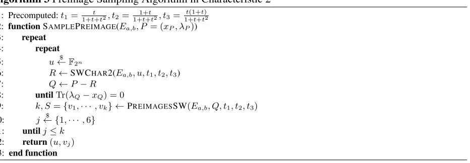
The details of our preimage sampling algorithm in characteristic 2 are described in Algorithm3witht fixed to a constant such thatt(t+ 1)(t2+t+ 1)6= 0,i.e.t6∈F4. Note that we make the choice to use the
λ-coordinates for efficiency reasons justified in§3.2. The rest of the section consists in describing the two subroutines SWCHAR2 and PREIMAGESSW, as well as in evaluating the overall complexity of Algorithm3.
3.1 The subroutine SWCHAR2
The first subroutine represents the binary Shallue–van de Woestijne algorithm and its pseudocode for our case is given as Algorithm4. Given a valueu∈F2n, it outputs the lambda coordinates of a point over the binary
elliptic curveEa,b.
Since the field inversion is by far the most expensive field operation (see [24] for experimental timings and Table2below), we have modified Algorithm2so that we have a single inversion ofcto perform. Indeed Algorithm2requires at most 4 field inversions: the first one at step 4 and the three others at step 6. However the parameters Xi and1/Xi forj = 1,2,3can be expressed usingc,1/cand some constants depending
ontwhich can be precomputed (see Table1). Note thatX3 can be computed asc·t3, or more efficiently
asX1+X2 +cbut this requires to keep in memoryX1 andX2. Finally this algorithm requires a single
field inversion, aQScomputation and some negligible field operations (multiplications, squarings and trace computations).
X1←t1·c 1/X1←1/t1·1/c
X2←t2·c 1/X2←1/t2·1/c
X3←X1+X2+c 1/X3←1/t3·1/c
Table 1.Efficient computation of valuesXiand1/Xifori = 1,· · ·3. The valuest1 = 1+t+tt 2,1/t1, t2 = 1+t+t1+t2,1/t2 and
1/t3= 1+t+t
2
t(1+t) can be precomputed, withta constant such thatt6∈F4.
3.2 The subroutine PREIMAGESSW
The second subroutine is useful to compute the number of preimages of the point Q = (xQ, λQ) by
Algorithm4. Its pseudocode is detailed as Algorithm5and refers to the steps 5 and 8 of Algorithm1. This subroutine is more complex due to the properties of the binary Shallue–van de Woestijne algorithm. More precisely, there is an order relation in Algorithm4: ifX1corresponds to ax-coordinate of a point over
Algorithm 3Preimage Sampling Algorithm in Characteristic 2
1: Precomputed:t1= 1+t+tt 2, t2= 1+t+t1+t2, t3= 1+t+tt(1+t)2
2: functionSAMPLEPREIMAGE(Ea,b, P = (xP, λP)) 3: repeat
4: repeat
5: u←$ F2n
6: R←SWCHAR2(Ea,b, u, t1, t2, t3)
7: Q←P−R
8: untilTr(λQ−xQ) = 0
9: k, S={v1,· · ·, vk} ←PREIMAGESSW(Ea,b, Q, t1, t2, t3) 10: j← {$ 1,· · ·,6}
11: untilj≤k
Algorithm 4Efficient Binary Shallue–van de Woestijne Algorithm
1: functionSWCHAR2(Ea,b, u, t1, t2, t3) 2: c←u2+u+a
3: c−1←1/c
4: forj= 1to 3do .Computehjand perform a trace test
5: Xj←tj·c .orX3←X1+X2+c
6: X−j←1/tj·c−1 .1/tjcan also be precomputed
7: hj←(X−j)2·b+Xj+a
8: ifTr(hj) = 0then .At least one of the three potential tests will succeed
9: x←Xj
10: λ←QS(hj) +x
11: break .Only take into account the first correct solution 12: end if
13: end for
14: return(x, λ) .Lambda coordinates of a point overEa,b 15: end function
the elliptic curve, then it will output this point, even ifX2andX3also correspond to a possiblex-coordinate.
Thus, the equality SWCHAR2(SWCHAR2−1(Xj)) =Xjis true forj= 1but not necessarly forj= 2,3. In
others words, forj= 2,3a solution of SWCHAR2−1(Xj)is not necessarily a preimage ofXj by SWCHAR2.
Starting from the equationsxQ = Xj(t, w) =c(w)·tj forj = 1,2,3, withc(w) =w2+w+a, the
main idea of Algorithm5consists in testing if there exists some values ofwwhich satisfy these equations. If one founds some candidates for w, one also has to verify if they really correspond to preimages by Algorithm4. From an equationxQ=Xj(t, w)we can obtain an equationw+w2=xQ/tj−a=αj(a, t)
which has 2 solutions ifTr(αj(a, t)) = 0and no solution otherwise. As an exampleα1(a, t)is equal to
xQ·(1 +t+t2)/t−a. The solutions are thenw10 = QS(αj(a, t))andw11=w01+ 1. There are thus at most
6 possible solutions for all values ofj. Now for the casesxQ =X2(t, w)andxQ =X3(t, w), it remains
to perform a verification. Actually, denotingw20 one of both solutions of the equationxQ =X2(t, w)if it
exists, the computation of SWCHAR2(w02)can result inX1(t, w02)instead ofX2(t, w02), and this happens
with probability1/2which is the probability thatTr(h1) = 0. The same result holds forxQ = X3(t, w),
however note that ifX3 is solution but notX1 thenX2 cannot be a solution since P3i=1Tr(g(Xi)) = 0
according to Theorem1. Thus the verification can focus only onX1.
Naive implementation of the verification. A simple way for implementing the verification would consist in computingQS(αj(a, t))forj = 2,3and then calling twice the subroutine SWCHAR2 (without the steps
referring toX2 andX3) for testing if the test on the trace is true or not. However this would require an
additional inversion per call to compute SWCHAR2. Moreover, with this naive implementation we have to
compute the half trace before testing if the result will be a preimage.
Efficient implementation of the verification. Since the verification focus only onX1as explained above, we
propose an efficient way to computeb/X12, which is required in order to performing the testTr(h1) = Tr(X1+
a+b/X12), without any field inversion. This trick is valuable when we are working in lambda coordinates. Our proposal has another advantage: we do not need to compute the solutions,i.e.w0 = QS(αj(a, t))and
w1 =w0+ 1, before to be sure that we will get two preimages. We thus save some quite expensive half trace
computations.
Consider the equation:
xQ=X2 =t2·c=t2·X1/t1 with c= QS(α2(a, t))2+ QS(α2(a, t)) +a.
X1 can be expressed ast1/t2 ·xQ, whose computation is negligible fort1/t2a precomputed value. Now
Algorithm 5Preimages Computation by Algorithm4 1: functionPREIMAGESSW(Ea,b, Q= (xQ, λQ), t1, t2, t3) 2: k←0
3: S← {}
4: forj= 1to 3do .FromxQ=Xj(t, w)...
5: αj←xQ·1/tj−a
6: ifTr(αj) = 0then ....Test if there are some solutions
7: ifj= 1then .ForX1, a solution is a preimage
8: w0←QS(αj)
9: w1←w0+ 1
10: k←2
11: S← {w0, w1}
12: else .ForX2, X3, a solution is not necessarly a preimage 13: X1←t1/tj·xQ
14: tmp←[(λQ−xQ)2+ (λQ−xQ)−xQ−a]·(tj/t1)2 . tmp=b/X12 15: h1←tmp+X1+a
16: ifTr(h1)6= 0then .Test ifX1would also be a correctx-coordinate
17: w0←QS(αj)
18: w1←w0+ 1
19: k←k+ 2
20: S←S∪ {w0, w1}
21: end if
22: end if
23: end if
24: end for
25: returnk, S . k: number of preimages,S: set of preimages 26: end function
we divide each term byX2and we evaluate the equation in the pointQ. We then obtain:
yQ
xQ
2
+ yQ xQ
=xQ+a+
b x2Q,
and finally:
b X12 =
t2
t1 2
·
yQ
xQ
2
+ yQ xQ
−xQ−a
.
Assuming that(t2/t1)2 is a precomputed constant, the computation ofb/X12 is not costly ifyQ/xQ does
not require an expensive operation. That is the case when we are working in λ-coordinates since λQ =
yQ/xQ+xQ. The same result obviously holds for the equationxQ =X3 by replacingt2witht3.
To conclude, Algorithm5 requires at most 3 QScomputations and some negligible field operations (multiplications, squarings and trace computations).
3.3 Operation counts
We conclude this section by evaluating the average number of operations needed to evaluate Algorithm3.
Proposition 1. An evaluation of Algorithm3on a uniformly random curve points requires, on average and up toO(2−n/2)variations,6field inversions,6point additions,9quadratic solver computations and some negligible operations such as field multiplications, field squares and trace computations.
verifying whetherTr(λQ−xQ) = 0. Indeed, all elements of the formQS(z)have zero trace by definition,
and the converse is true for reasons of dimensions. The success probability of this test is exactly1/2since Qis a uniformly random curve point. We thus have on average2field inversions,2point additions and2 quadratic solver computations for the internal loop (steps 4 to 8).
The complexity of the external loop demands to evaluate the probabilities for having 0, 2, 4 or 6 preimages ofQ. Since all tests on the trace in Algorithm5succeed, independently, with probability1/2up toO(2−n/2) variations7, these probabilities are then, again up toO(2−n/2)variations,9/32for0preimage,15/32for2
preimages,7/32for4preimages, and1/32for 6 preimages. Thus, the probability for exiting the external loop is equal to0·9/32 + 1/3·15/32 + 2/3·7/32 + 1·1/32 = 1/3. These probabilities also hold for evaluating the average cost of an iteration of PREIMAGESSW in term of quadratic computations. With probability15/32 one such computation will be performed and so on. As a consequence, one iteration of PREIMAGESSW cost on average 15·1+732·2+1·3 = 1quadratic solver computation.
To sum up, Algorithm3requires on average3·2field inversions,3·2additions of points and3·(2 + 1)
quadratic solver computations, up toO(2−n/2variations. ut
Note that the efficiency of this algorithm can be improved further by choosing a sparse value ofband a value oftthat yields sparse precomputed constants. Many of the field multiplications will then be computed faster.
4 Implementation aspects
Our software implementation targets modern Intel Desktop-based processors, making extensive use of the recently introduced AVX instruction set [16] accessible through compiler intrinsics. The curve choice is the GLS binary curve(λ2+λ+a)x2 =x4 +brepresented inλ-coordinates and defined over the quadratic extensionF2254. The extension is built by choosing the irreducible trinomialg(u) =u2+u+ 1over the base
fieldF2127 defined with the irreducible trinomialf(z) =z127+z63+ 1. In this set of parameters, a field
elementais represented asa=a0+a1u, witha0, a1 ∈F2127.For simplicity, parametertis chosen to be
a random subfield element, allowing the computational savings by sparse multiplications described in the previous section.
Squaring and multiplication. Field squaring closely mirrors the vector formulation proposed in [3], with coefficient expansion implemented by table lookups performed through byte-shuffling instructions. The table lookups operate on registers only, allowing a very efficient constant-time implementation. Field multiplication is natively supported by the carry-less multiplier (PCLMULQDQ instruction), with the number of word multiplications reduced through application of Karatsuba formulae, as described in [26]. Modular reduction is implemented with a shift-and-add approach, with careful choice of aligning vector word shifts on multiples of 8, to explore the faster memory alignment instructions available in the target platform.
Half-trace computation. For an odd extension degreem, the half-trace functionHTr :F2m →F2mis defined
byHTr(c) =P(im=0−1)/2c22i and computes a solutionc∈F2mto the quadratic equationλ2+λ=c+ Tr(c).
In a quadratic extension, the equationλ2 +λ = c+ Tr(c) can be solved for c = c0 +c1u ∈ F22m by
computing two half-traces inF2m, as described in [20]. First, solveλ2
1+λ1=c1to obtainλ1, and then solve
λ2
0+λ0 =c0+c1+λ1+ Tr(c0+c1+λ1)to obtain the solutionλ=λ0+ (λ1+ Tr(c0+c1+λ1))u. This
approach is very efficient for variable-time implementations and only requires two half-trace computations in the base field, where each half-trace computation employs a large precomputed table of28· dm
8efield
elements [24]. 7
A more naive approach evaluates the function by alternatingm−1consecutive squarings and(m−1)/2 additions, with the advantage of taking constant-time (if squaring and addition are also constant-time, as in the case here). We derive a faster way to compute the half-trace function in constant-time over quadratic extension fields. Applying the naive approach to a quadratic extension allows a significant speedup due to the linear property of half-trace, by reducing the cost to essentially one constant-time half-trace computation over the base field. By considering thatλ21+λ1=c1has a solutionλ1 ∈F2m, we always haveTr(λ1) = Tr(c1) = 0.
This simplifies the expression above toλ20+λ0 =c0+c1+λ1+ Tr(c0). Substitutingd=c0+ Tr(c0), the
expression forλ0becomes:
λ0 =
(m−1)/2 X
i=0
(d+c1+λ1)2 2i
=
(m−1)/2 X
i=0
d+c1+
(m−1)/2 X
j=0
c212j
22i
.
The expansion of the inner sum allows the interleaving of the consecutive squarings. The analysis can be split in two cases, depending on the format of the extension degreem:
λ0 =
c0+
bm/4c−1 X
i=0
(c160 +d4+c41+c81)24i ifm≡1 (mod 4) bm/4c
X
i=0
(c0+d4+c21+c41)2 4i
ifm≡3 (mod 4).
The valueλ1can then be computed asλ1=λ20+λ0+d+c1, for a total of approximatelymsquarings
andm/4additions, a cost comparable to a single constant-time half-trace in the base field.
Inversion. Field inversion is implemented by two different approaches based on the Itoh-Tsuji algorithm [21]. This algorithm computesa−1 = a(2m−1−1)2, as proposed in [19], with the cost ofm−1squarings and a number of multiplications determined by the length of an addition chain for m −1. For a variable-time implementation, the squarings for each2i-power involved can be converted into a multi-squaring [8], implemented as a trade-off between space consumption and execution time. Each multi-squaring table requires the storage of24· dm4efield elements. A constant-time implementation must perform consecutive squarings and cannot benefit considerably from a precomputed table of field elements without introducing variance in the memory hierarchy latency potentially exploitable by an intrusive attacker.
Point addition. The last performance-critical operation to be described is the point addition in λ-affine coordinates. A formula for adding pointsP = (xP, yP)andQ= (xQ, yQ)on the curve is proposed in [24],
with associated cost of 2 inversions, 4 multiplications and 2 squarings :
xP+Q =
xP ·xQ(λP +λQ)
(xP +xQ)2
, λP+Q =
xQ·(xP+Q+xP)2
xP+Q·xP
+λP + 1.
Simple substitution of xP+Q in the computation of λP+Q gives faster new formulas. By unifying the
denominators, one field inversion can be traded for 2 multiplications in the formulas below, with associated cost of 1 inversion, 6 multiplications and 2 squarings:
xP+Q=
xP ·xQ(λP +λQ)2
(xP +xQ)2(λP +λQ)
, λP+Q=
(xP +xQ)2+xQ·(λP +λQ)
2
(xP +xQ)2(λP +λQ)
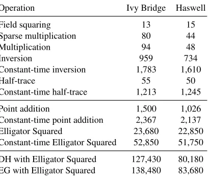
Operation Ivy Bridge Haswell
Field squaring 13 15
Sparse multiplication 80 44
Multiplication 94 48
Inversion 959 734
Constant-time inversion 1,783 1,610
Half-trace 55 50
Constant-time half-trace 1,213 1,245
Point addition 1,500 1,026
Constant-time point addition 2,367 2,137 Elligator Squared 23,680 22,850 Constant-time Elligator Squared 52,850 51,750 DH with Elligator Squared 127,430 80,180 EG with Elligator Squared 138,480 83,680
Table 2.Timings for Elligator Squared and underlying field arithmetic in two Intel platforms. Results are in clock cycles and were taken as the average of104
executions with random inputs. DH/EG results refer to generating a random point for ECDH (fixed-base) or ElGamal encryption (variable-base) using the constant-time, timing-attack protected scalar multiplication from [24], and computing its Elligator Squared representation with variable-time arithmetic.
5 Experimental results
The implementation was realized with help from the latest version of the RELIC toolkit [2]. Random number generation was implemented with the recently introducedRDRANDinstruction [12]. Software was compiled with a prerelease version of GCC 4.9 available in the Arch Linux distribution with flags for loop unrolling, aggressive optimization (-O3level) and specific tuning for the Sandy/Ivy Bridge microarchitectures. Table
2presents timings in clock cycles for field arithmetic and Elligator Squared in two different platforms – an Intel Ivy Bridge Core i5 3317U 1.7GHz and a Haswell Core i7 4770K 3.5GHz. The timings were taken as the average of104executions, with TurboBoost and HyperThreading disabled to reduce randomness in the results.
The constant-time implementation results are mostly for reference: indeed, since the Elligator Squared operation is efficiently invertible, there is no strong reason to compute it in constant time: timing information does not leak secret key data like in the case of a scalar multiplication. However, timing information could conceivably help an active distinguishing attacker; the corresponding attack scenarios are far-fetched, but the paranoid may prefer to choose constant-time arithmetic as a matter of principle.
6 Comparison of Elligator 2 and Elligator Squared on Prime Finite Fields
We have implemented Elligator 2 [6] and the corresponding Elligator Squared construction on Curve25519 [4] using the fast arithmetic provided by Bernstein et al. as part of the publicly available implementation of Curve25519 and Ed25519 [5] in SUPERCOP, in order to compare the two proposed methods on Edwards curves in large characteristic (and to see how they both perform compared to our binary implementation).
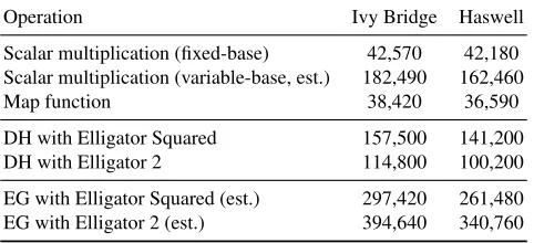
Operation Ivy Bridge Haswell Scalar multiplication (fixed-base) 42,570 42,180 Scalar multiplication (variable-base, est.) 182,490 162,460
Map function 38,420 36,590
DH with Elligator Squared 157,500 141,200 DH with Elligator 2 114,800 100,200 EG with Elligator Squared (est.) 297,420 261,480 EG with Elligator 2 (est.) 394,640 340,760
Table 3.Timings for Elligator Squared and Elligator 2 on Curve25519. Results are in clock cycles and were taken as the average of
104executions with random inputs. DH/EG are as in Table2.
conversely. Elligator will thus tend to have an edge for protocols using fixed base point scalar multiplication, such as ECDH key generation or ECDSA signatures, whereas Elligator Squared will perform better for protocols using variable base point scalar multiplication, like ElGamal encryption.
This is confirmed by our implementation results, as reported in Table3, which are 35–40% in favor of Elligator in the fixed-base case (DH) but 30–35% in favor of Elligator Squared in the variable-base case (EG). Note that the variable-base scalar multiplication results are estimates based on the SUPERCOP performance numbers onhaswellandhydra2. A comparison with Table2shows that the binary curve approach is 25% to 200% times faster than the fastest Curve25519 implementation.
References
1. ANSSI. Publication d’un param´etrage de courbe elliptique visant des applications de passeport ´electronique et de l’administration ´electronique franc¸aise. http://www.ssi.gouv.fr/fr/anssi/publications/publications- scientifiques/autres-publications/publication-d-un-parametrage-de-courbe-elliptique-visant-des-applications-de.html, November 2011.
2. D. F. Aranha and C. P. L. Gouvˆea. RELIC is an Efficient LIbrary for Cryptography. http://code.google.com/p/relic-toolkit/.
3. Diego F. Aranha, Julio L´opez, and Darrel Hankerson. Efficient software implementation of binary field arithmetic using vector instruction sets. InLATINCRYPT, pages 144–161, 2010.
4. Daniel J. Bernstein. Curve25519: New Diffie-Hellman speed records. In Moti Yung, Yevgeniy Dodis, Aggelos Kiayias, and Tal Malkin, editors,Public Key Cryptography, volume 3958 ofLecture Notes in Computer Science, pages 207–228. Springer, 2006. 5. Daniel J. Bernstein, Niels Duif, Tanja Lange, Peter Schwabe, and Bo-Yin Yang. High-speed high-security signatures. J.
Cryptographic Engineering, 2(2):77–89, 2012.
6. Daniel J. Bernstein, Mike Hamburg, Anna Krasnova, and Tanja Lange. Elligator: Elliptic-curve points indistinguishable from uniform random strings. In Virgil Gligor and Moti Yung, editors,ACM CCS, 2013.
7. Daniel J. Bernstein, Mike Hamburg, Anna Krasnova, and Tanja Lange. Elligator: Software.http://elligator.cr.yp. to/software.html, August 2013.
8. Joppe W. Bos, Thorsten Kleinjung, Ruben Niederhagen, and Peter Schwabe. ECC2K-130 on Cell CPUs. InAFRICACRYPT, pages 225–242, 2010.
9. Eric Brier, Jean-Sebastien Coron, Thomas Icart, David Madore, Hugues Randriam, and Mehdi Tibouchi. Efficient indifferentiable hashing into ordinary elliptic curves. Cryptology ePrint Archive, Report 2009/340, 2009.http://eprint.iacr.org/. Full version of [10].
10. Eric Brier, Jean-S´ebastien Coron, Thomas Icart, David Madore, Hugues Randriam, and Mehdi Tibouchi. Efficient indifferentiable hashing into ordinary elliptic curves. In Tal Rabin, editor,CRYPTO, volume 6223 ofLecture Notes in Computer Science, pages 237–254. Springer, 2010.
11. Certicom Research. SEC 2: Recommended elliptic curve domain parameters, Version 2.0, January 2010.
12. Intel Corporation. Intel Digital Random Number Generator (DRNG). https://software.intel.com/sites/ default/files/managed/4d/91/DRNG_Software_Implementation_Guide_2.0.pdf.
14. Reza Rezaeian Farashahi, Pierre-Alain Fouque, Igor Shparlinski, Mehdi Tibouchi, and Jos´e Felipe Voloch. Indifferentiable deterministic hashing to elliptic and hyperelliptic curves.Math. Comp., 82(281), 2013.
15. FIPS PUB 186-3.Digital Signature Standard (DSS). NIST, USA, 2009.
16. N. Firasta, M. Buxton, P. Jinbo, K. Nasri, and S. Kuo. Intel AVX: New frontiers in performance improvement and energy efficiency. White paper.http://software.intel.com/.
17. Pierre-Alain Fouque, Antoine Joux, and Mehdi Tibouchi. Injective encodings to elliptic curves. In Colin Boyd and Leonie Simpson, editors,ACISP, volume 7959 ofLecture Notes in Computer Science, pages 203–218. Springer, 2013.
18. Pierre-Alain Fouque and Mehdi Tibouchi. Indifferentiable hashing to Barreto-Naehrig curves. In Alejandro Hevia and Gregory Neven, editors,LATINCRYPT, volume 7533 ofLecture Notes in Computer Science, pages 1–17. Springer, 2012.
19. Jorge Guajardo and Christof Paar. Itoh-Tsujii inversion in standard basis and its application in cryptography and codes.Des. Codes Cryptography, 25(2):207–216, 2002.
20. Darrel Hankerson, Koray Karabina, and Alfred Menezes. Analyzing the Galbraith-Lin-Scott point multiplication method for elliptic curves over binary fields.IEEE Trans. Computers, 58(10):1411–1420, 2009.
21. Toshiya Itoh and Shigeo Tsujii. A fast algorithm for computing multiplicative inverses inGF(2m)using normal bases. Inf.
Comput., 78(3):171–177, 1988.
22. M. Lochter and J. Merkle. Elliptic curve cryptography (ECC) Brainpool standard curves and curve generation. RFC 5639 (Informational), March 2010.
23. Bodo M¨oller. A public-key encryption scheme with pseudo-random ciphertexts. In Pierangela Samarati, Peter Y. A. Ryan, Dieter Gollmann, and Refik Molva, editors,ESORICS, volume 3193 ofLecture Notes in Computer Science, pages 335–351. Springer, 2004.
24. Thomaz Oliveira, Julio L´opez, Diego F. Aranha, and Francisco Rodr´ıguez-Henr´ıquez. Two is the fastest prime: lambda coordinates for binary elliptic curves.J. Cryptographic Engineering, 4(1):3–17, 2014.
25. Andrew Shallue and Christiaan van de Woestijne. Construction of rational points on elliptic curves over finite fields. In Florian Hess, Sebastian Pauli, and Michael E. Pohst, editors,ANTS, volume 4076 ofLecture Notes in Computer Science, pages 510–524. Springer, 2006.
26. Jonathan Taverne, Armando Faz-Hern´andez, Diego F. Aranha, Francisco Rodr´ıguez-Henr´ıquez, Darrel Hankerson, and Julio L´opez. Speeding scalar multiplication over binary elliptic curves using the new carry-less multiplication instruction. J. Cryptographic Engineering, 1(3):187–199, 2011.
27. Mehdi Tibouchi. Elligator Squared: Uniform points on elliptic curves of prime order as uniform random strings. In Nicolas Christin and Reihaneh Safavi-Naini, editors,Financial Cryptography, Lecture Notes in Computer Science. Springer, 2014. To appear.
28. Zachary Weinberg, Jeffrey Wang, Vinod Yegneswaran, Linda Briesemeister, Steven Cheung, Frank Wang, and Dan Boneh. StegoTorus: a camouflage proxy for the Tor anonymity system. In Ting Yu, George Danezis, and Virgil D. Gligor, editors,ACM CCS, pages 109–120. ACM, 2012.
29. Eric Wustrow, Scott Wolchok, Ian Goldberg, and J. Alex Halderman. Telex: Anticensorship in the network infrastructure. In
USENIX Security Symposium. USENIX Association, 2011.
30. Adam L. Young and Moti Yung. Space-efficient kleptography without random oracles. In Teddy Furon, Franc¸ois Cayre, Gwena¨el J. Do¨err, and Patrick Bas, editors,Information Hiding, volume 4567 ofLecture Notes in Computer Science, pages 112–129. Springer, 2007.