Dynamic Clustering in Sensor Networks using
HMM and Neuro Computation
Veena k.N.#1, Vijaya Kumar B.P.*2 #1
Department of Telecommunication Engg, J.N.N. College of Engineering, Shimoga, India
*2
Department of Telecommunication Engg., M.S.Ramaiah Institute of Technology, Bangalore, India
Abstract— Most important challenge in Wireless Sensor
Networks is to improve the operational efficiency in highly resource constrained environment based on dynamic and unpredictable behavior of network parameters and applications requirement. In this paper we have proposed a technique of clustering and analysis, to study the system behavior with respect to network parameters and applications requirement. The technique involves in the adoption of Fuzzy logic and Hidden Markov Model for the analysis of sensor node parameters and Neuro computation for clustering. The simulations are carried out to evaluate the performance of the proposed method with respect to different parameters of sensor networks and applications requirement.
Keywords
—
Wireless Sensor Networks, Clustering, Hidden Markov Model, Neural networks, Fuzzy logic.I. INTRODUCTION
In the recent years, Wireless Sensor Networks (WSNs) has found a wide variety of applications and systems with vastly varying requirements and characteristics. As a result, the complexities of the system design issues and their requirement have increased with respect to hardware and software. Integrating sensor nodes into sophisticated sensing, computational and communication infrastructures to form wireless sensor networks will have a significant impact on a wide array of applications ranging from military, scientific, industrial, health-care and domestic services. Various applications of WSN are Telemedicine, Habitat monitoring, Structure health monitoring, Active Volcano, Seismic monitoring, and Avalanche Victims. Wireless sensor networks are usually a large number of sensor nodes, which are tiny, compact and low cost embedded devices, which can be readily deployed in various types of unstructured environments within predefined and specified area or sometimes an approximate area of interest, either inside the phenomenon or very close to it. Efficiency of such systems would improve by providing distributed, localized and energy efficient techniques. Here the sensor nodes have native capabilities to detect the nearest neighbors and help to develop an ad-hoc network through a set of well-defined protocols. This leads to the existence of clusters of nodes, which can enhance the network operations under network management, processing and aggregation of sensor data. Therefore there are many advantages with clustering and their analysis based on the system parameters and applications requirement. The systematic clustering by choosing the key parameters and response to their dynamic behavior in
resource constrained sensor networking environment will be a challenging and complex issue.
In this work, we have proposed a technique of clustering and analysis to study the dynamic behavior of the system that includes sensor network parameters and applications requirement. This paper is extension of our previous paper[1]. The method involves the Fuzzy Logic in fuzzifyng the sensor node parameters. Hidden Markov Model (HMM) is used in estimating a sensor node suitable for a particular application. We have used Kohonen Self Organization Map Neural Network (KSOM-NN) [2] as Computational Intelligence for clustering.
The organization of the paper is as follows. A brief discussion on some of the related works is explained in section II. Section III explains the proposed Dynamic clustering model. Concept of clustering is explained in section IV. The description of the proposed clustering algorithm is narrated in section V. Simulation and results are described in section VI and concluding remarks are given in section VII.
II. RELATED WORKS
A distributed, randomized clustering algorithm [9] to organize the sensors in a wireless sensor network into clusters is discussed. The algorithms generate a hierarchy of cluster heads and observe that the energy savings increase with the number of levels in the hierarchy. The Linked Cluster Algorithm [10] where a node becomes the cluster head, if it has the highest identity among all the nodes within one hop of itself or among its neighbors is presented. Budget-based clustering approaches [11], message efficient distributed clustering [12] are proposed, involving autonomous sensor network clusters of bounded size by keeping lower overall message complexity. In [13] determination of the optimal number of clusters in an observation area is implemented.
III.DYNAMIC CLUSTERING MODEL
Fig. 1 Dynamic Clustering model
Dynamic clustering model using Neuro-Fuzzy Technique and Hidden Markov Model is shown in fig 1. The sensor data readings are fuzzified. Ex: Power present in sensor nodes, memory available and processing speed of sensor nodes are given to fuzzifier. The fuzzifier assigns monitoring coefficients for each sensor nodes according to predefined fuzzy rules. Ex: Monitoring coefficients for sensor node which can be used for critical monitoring, used for event monitoring, continuous and cannot be used for monitoring because of very low power availability. These coefficients are then given HMM to estimate the application coefficient for each sensor node that is suitable for various applications. Ex: A senor node can be suitable for Precision agriculture, Environmental monitoring, Habitat monitoring, Disaster monitoring etc. These coefficients of sensor node are given to KSOM neural network for clustering. Depending on the application requirement, cluster of sensor nodes suitable for Precision agriculture, environmental monitoring, seismic monitoring, habitat monitoring and disaster monitoring are obtained.
IV.CLUSTERING IN WIRELESS SENSOR NETWORKS
Clustering is the architecture of choice as it keeps the traffic local and sensor nodes would send information only
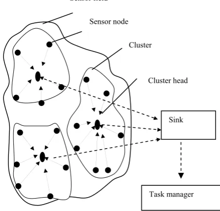
to the nearby cluster head within a fixed radius. Clustering sensor nodes are advantageous because they conserve limited energy resources (power) and improve energy efficiency. In a cluster, each cluster will contain a cluster head. Each cluster head gathers information from its group of sensors, perform data aggregation and relay only relevant information to the sink as shown in fig 2. By aggregating the information from individual sensors, can abstract the characteristics of network topology along with applications requirement and it also reduces the bandwidth. This provides scalability and robustness for the network and increases the lifetime of the system.
Fig. 2 Clustered Wireless Sensor Network
V. PROPOSED CLUSTERING ALGORITHM
We propose a technique for clustering and cluster analysis to study the behavior and operation of WSN with respect to network parameters and applications requirement. There are application parameters, which will have the influence over the resources available in WSN. Hence there is a need to understand how WSN behaves keeping its resource-constrained environment with respect to applications requirement. For clustering we have adopted the computational intelligence technique, which deals with the numerical data and does not use knowledge in the AI sense and exhibits computational adaptivity with fault tolerance [14]. This study is essential to enhance the clarity in understanding the behavior of WSN parameters pertaining to the specific applications to improve the operational efficiency. The proposed clustering algorithm is given below.
Algorithm 1. Proposed Dynamic Clustering Algorithm Begin
1. The sensor node parameters such as memory, power available, processing speed of each sensor nodes is considered.
2. These sensor node parameters are fuzzified using fuzzy logic with fuzzy rules as given in Table1.
--- Fuzzifer
HMM
KSOM for clustering
Sensor node parameters (power, memory, processing
Cluster nodes for suitable environmental monitoring
Cluster of nodes suitable for habitat monitoring Monitoring coefficients of nodes
Application coefficient
Cluster of nodes suitable for Precision agriculture monitoring
Sink
Task manager Sensor field
Sensor node
Cluster
3. The fuzzifier assigns monitoring coefficient for each node, depending on its power availability, memory availability, processing speed.
4. These monitoring coefficients are given to HMM to estimate application coeffi cient for each sensor node.
5. These application coefficients are given to KSOM neural network to obtain clusters depending on the application requirement.
End
5.1 Fuzzy Logic
The model using fuzzy logic [15] consists of a fuzzifier, fuzzy rules, fuzzy inference engine, and a defuzzifier. Input variables used are sensor node parameters such as power available in sensor node, memory and processing speed. Membership function and Fuzzy rules are applied to the sensor node parameters. The membership functions developed and their corresponding linguistic states are represented in Table 1 and fig 3 through fig 6. The Fuzzifier assigns the monitoring coefficients for each sensor nodes.
Fig. 3 Membership function for power present in sensor node
Fig. 4 Membership function for memory available in sensor node
Fig. 5 Membership function for processing speed in sensor node
Fig. 6 Membership function for monitoring coefficient of sensor node
TABLE 1 FUZZY RULES
Power Memory Processing
speed Monitoring coefficient
1 low low low Not used
2 medium medium medium critical 3 medium high medium event 4 medium medium high event
5 medium high high event
6 high high medium continuous 7 high medium high continuous
8 high high high continuous
Sensor nodes which have high power, memory and processing speed can be used for continuous monitoring. Sensor nodes with medium power, high memory and high processing speed can be used for event monitoring, sensor nodes with medium power and low memory and processing speed can be used for critical monitoring. Sensor nodes with low power and low memory and low processing speed cannot be used for monitoring.
5.2 Hidden Markov Model
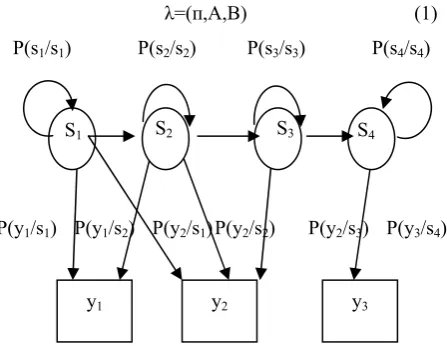
A Hidden Markov Model (HMM)[16] is a statistical Markov model in which the system being modeled is assumed to be a Markov process with unobserved (hidden) states. A Hidden Markov Model is shown in the fig 7 and it is denoted by equation 1.
λ=(п,A,B) (1)
Fig. 7 General Architecture of a Hidden Markov Model
s- states (application coefficients); y-observations (monitoring coefficients); a- State transition probabilities; b-output probabilities;
N applications of WSN are modeled as N hidden states, with S = {S1, S2, …, SN} the set of hidden states, in our case
N=4. y is the number of observable parameters, y monitoring coefficients of sensor nodes are considered, with y = { y1, y2, …, yT} the set of observable parameters, in
our case m=3.
A={aij}, the transition probabilities between the hidden
states Si and Sj, aij =P[Sj(t+1)| Si (t)], 0≤ i, j≤ N.
B = {bjk} - the probabilities of the observable states yk in
hidden states Sj, bj (k) = P[yk(t)| Sj(t)], 0 ≤ j ≤ N, 0 ≤ k ≤ T.
0 40 50 80 90 128 in kB
low medium high
Not used critical event continuous
0 0.1 0.2 0.25 0.3 0.45 0.5 1
0 1.0 1.2 2.0 2.5 3 in mw
low medium high
y1 y2 y3
S3
S2 S4
P(s1/s1)
S1
P(s2/s2) P(s3/s3) P(s4/s4)
P(y1/s1) P(y1/s2) P(y2/s1) P(y2/s2) P(y2/s3) P(y3/s4)
0 3.5 4 4.5 5 7.3 in
The following transition state matrix probabilities and emission probabilities are considered for HMM computation. A= 1 0 0 0 2 . 0 8 . 0 0 0 0 2 . 0 8 . 0 0 0 0 2 . 0 8 . 0 B= 1 0 0 0 1 0 0 4 . 0 6 . 0 0 3 . 0 07
π = The initial hidden state probabilities, пi = P[ S i], 0≤ i ≤
N.
j
ij for all i
a 1 ,
k
jk for all j
a 1
5.2.1 Algorithms of HMM
This section introduces the three main algorithms for the solution of the standard problems of HMM is given. They are
The Decoding Problem:
Given a sequence of emissions yT over time T and a
HMM with complete model parameters, meaning that transition and emission probabilities are known, this problem computes the most probable underlying sequence ST of hidden states that led to this particular observation.
The Evaluation Problem:
Here the HMM is also given with complete model parameters, along with a sequence of emissions yT. In this
problem the probability of a particular yT to be observed
under the given model has to be determined.
The Learning Problem:
The elemental structure of the HMM is given. Given one or more output sequences, this problem computes the model parameters A, B. i.e the parameters of the HMM have to be trained.
Forward Algorithm:
The Forward algorithm is gives the solution for the Evaluation Problem. Forward algorithm and time reversed version of backward algorithm is discussed.
) (t i
is the probability that the model is in state Si(t) and
has generated the target sequence upto step t. i(t)is the
probability that the model is in state Si(t) and will generate
the remainder of the given target sequence from t+1 to T.
otherwise ) t ( y b a ) 1 t(0andj initial state t
10 t 0 andj initial state )
t (
jk
i i ij
j
Algorithm 2: Forward Algorithm Begin
1. Initialize t=0, aij, bjk, observed sequence y
T, (0)
j
2. For tt+1
3.
N
1
i i ij
jk
j(t) b y(t) (t 1)a
4. until t=T
5. Return P(yT) 0(T)for the final state End
Algorithm 3:Backward Algorithm Begin
1. Initialize j(T), tT, aij, bjk, observed sequence yT
2. For tt-1
3. (t) (t 1)a bjky(t 1) N
1
j j ij
j
4. until t=1
5. Return P(yT) i(0)for the known initial state End
Decoding algorithm:
The Decoding problem is solved by the Decoding algorithm, which is sometimes called Viterbi algorithm.It is used to find the most likely sequence of hidden states to have generated a particular output sequence, given the model parameters.
Algorithm 4: Decoding Algorithm Begin
1. Initialize Path {}, t0 2. For tt+1
3. jj+1 4. for jj+1
5.
N i ij j jk
jt b yt t a
1 ) 1 ( ) ( ) (
6. until j=N 7.
j
j t
j'argmax ()
8. Append '
j
s to path
9. until t=T 10. Return path End
Baum-Welch algorithm
The Baum-Welch algorithm, also known as Forward-Backward Algorithm, is used for Learning Problem.
otherwis ) 1 t( y b a ) 1
t( s t() s and t T 10 s t() s and t T )
t(
jk j j ij
0 i
0 i j
The probability of transition between si(t-1) and si(t) give
the model generated the entire training sequence yT by any
path is
)
|
T
y
(
P
)
t
(
j
jk
b
ij
a
)
1
t
(
i
)
t
(
ij
Here λ denotes the HMMs model parameters (aij and bjk), and therefore p(VT|λ) is the probability that the model
generated VT. Hence the auxiliary quantity is the
probability of a transition from Si(t − 1) to Si(t), under the condition that the model generated VT .
) 2 ( ) t ( ) t ( a T 1 t k ik
Numerator is the expected number of transitions between state Si(t-1) and Si(t), Denominator is the total expected
number of transitions from Si.
)
3
(
)
t
(
)
t
(
b
T1 t l jl
T
k y ) t ( y , 1
t l jl
jk
It is the ratio between frequency that any particular symbol yk is emitted and that for any symbol.
Algorithm 5: Baum Welch Algorithm Begin
1. Initialize aij , bik, training sequence yT, z0, convergence criterion.
2. do zz+1
3. Compute a(z)
from a(z-1) and b(z-1) by eqn. 2
4. Compute b(z)
from a(z-1) and b(z-1) by eqn. 3
5. aij(z) ( 1)
z aij
6. bjk(z) ( 1)
z bjk
7. Until max[ ( ) ( 1), ( ) ( 1)]
, ,
a z b z a z
z
aij ij jk jk
k j i
<
8. Return aijaij(z); bjk bjk(z)
End
5.3 Kohonen Self Organizing Map-Neural Network
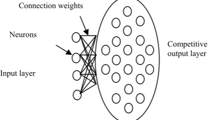
Clustering computation is carried out using Kohonen Self–Organizing Map Neural Networks (KSOM-NN) algorithm to cluster the sensor nodes depending on the parameters of interest. The KSOM-NN is competitive, feed forward type and unsupervised training neural network. They have the capability of unsupervised learning and self-organizing properties, is able to infer relationships and learn more as more inputs are presented to it. The Application coefficient of each sensor nodes is considered to cluster sensor nodes using Kohonen Self-Organizing Map Neural Networks. Cluster of sensor nodes suitable for various applications are formed. The fig 8 shows a typical example of a KSOM-NN [17] with 4 input and 20 output neurons.
Fig. 8 A typical KSOM-NN model with 4 input and 20 output neurons
Let the input pattern be: I = (I1, I2,.,I|V|), where there are
|V| input neurons in the input layer. Now suppose there are Q neurons in the output (competitive) layer, let Oj be the jth
output neuron. So the whole of the output layer will be: O= (O1,O2,.,OQ) for each output neuron Oj there are |V|
incoming connections from the |V| input neurons. Each
connection has a weight value W. So, for any neuron Oj on
the output layer the set of incoming connection weights are: wj=(wj1,wj2,.,wj|v|). The Euclidean distance value Dj of a
neuron Oj in the output layer, whenever an input pattern I is
presented at the input layer, is:
|V.|
1 i
2 ) ji W i I (
j
D (4)
The competitive output neuron with the lowest Euclidean distance at this stage is the closest to the current input pattern, called as winning neuron, Oc. The fig. 9 shows an
example of a neighborhood around a winning neuron Oc.
Fig.9 A 4X4 Kohonen grid showing the size of neighborhood influence around neuron Oc.
As shown in figure 3, the neighborhood size and weight updating computation use the following equations (4) and (5). The size of the neighborhood h, starts with a big enough size and decreases with respect to learning iterations such that:
ht=h0(1-t/T) ---(5)
Where, ht denotes the actual neighborhood size, h0
denotes the initial neighborhood size, t denotes the current learning epoch and T denotes the total number of epochs to be done. Where an epoch is when the network has swept through all the input patterns of every sensor node once. During the learning stage, the weights of the incoming connections of each competitive neuron in the neighborhood of the winning one are updated, including the winning neuron.
The overall weights update equation is: Wjnew= Wjold + α (I - Wjold) ---(6)
if unit Oj is in the neighborhood of winning unit Oc.
Where, α is the learning rate parameter, typical choices are in the range [0.2 . . 0.5]. A learning algorithm I for clustering is summarized as follows.
Algorithm 6: Learning algorithm for Clustering
Begin
1. Assign random values to the connection weights, W in the range (0, 1);
2. Select an input pattern ie., parameters of the sensor nodes.
3. Determine the winner output neuron Oc using equation (4);
4. Perform a learning step affecting all neurons in the neighborhood of Oc by updating the connection
weights using equation (5); and update ht and continue with step 2 until no noticeable changes in the connection weights are observed for all the input patterns.
5. Stop End.
Input layer Neurons
Connection weights
Competitive output layer
VI.SIMULATION AND RESULTS
In order to evaluate the performance of the proposed technique simulation is carried out based on sensor node characteristic features such as power present in sensor nodes, memory available and processing speed. Fuzzy logic is used to fuzzify the sensor node parameters. The fuzzifier gives the membership function coefficients for monitoring. Then the monitoring coefficients are given HMM to estimate the application coefficient for each sensor node. These application coefficients are given to KSOM to obtain dynamic clusters depending on the application requirement.
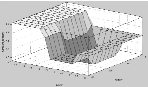
Clustering of sensor node using KSOM-NN is computed for various numbers of nodes by taking monitoring coefficients of sensor node. The clustering implementation is carried out using C++ programming language by defining suitable classes and structures. Simulation experiments are carried out rigorously by taking different number of nodes in sensor networks, i.e., 100 to 1000. The simulation program is run for many iterations until they converge to stable clusters. A plot of monitoring coefficients for various parameter of a sensor node such as power, memory available and processing speed is shown in fig 10, and fig 11. The result shows that as power, memory and processing speed is high for a sensor node, then monitoring coefficients generated is also high. Such type of sensor node can used for continuous monitoring. If power present in a sensor node is very low, then monitoring coefficient generated is low such sensor nodes cannot be used for monitoring purpose. These results help us in analyzing, whether a node is capable of monitoring a phenomenon or not and how well it can monitor an area of interest.
Fig. 10Monitoring coefficients of sensor node with respect to power and processing speed.
Fig. 11 Monitoring coefficients for sensor node with respect to power and memory
Fig. 12 Cluster formed with respect to application requirement
Fig. 13 Time for computation to form clusters with respect to parameters of sensor node
The fig 12 shows the number of clusters formed with respect to application coefficient of sensor nodes in WSN. The results show that the number of clusters formed is dependent of the number of parameters of sensor nodes chosen and the application requirement. These results are essential and can be easily used in various applications depending on the critical region of interest. For example, nodes which can be used for continuous monitoring are suitable for precision Agriculture, and nodes which can be used for event monitoring are suitable for monitoring of seismic area. The computation time for clustering is measured with respect to application and number of sensor nodes as shown in fig 13. These results show on how the individual parameters affect the formation of cluster and its size. These results would be used in real time decision making applications and in adaptive systems.
VII. CONCLUSION
In this work we have proposed a technique for clustering and their analysis to study the dynamic behavior of the cluster formation based on the system parameters and application requirements. The technique involves the adoption of computational intelligence to form clustering and analyzing sensor node parameters in WSN. We have used computational intelligence, Neuro-Fuzzy techniques and Hidden Markov Model for the above computations. The simulations are carried out to evaluate the performance of the proposed method with respect to different parameters of sensor networks and applications requirement. Since we are analyzing and estimating sensor nodes depending on the application requirement, proactive decisions can be taken. The decisions can be redeployment of sensor nodes, when we estimates some of the sensor cannot be used for monitoring because of very low power, or sensor nodes are
0 0.2 0.4 0.6 0.8 1 1.2 1.4 1.6 1.8 2
1 2 3 4
no. of parametrs
ti
m
e
fo
r
c
o
m
p
u
tat
io
n
n=1000
n=500
n=100
0 1 2 3 4 5 6 7 8 9
1 2 3 4
No. of parameters
N
o
. of
c
lus
te
rs
f
o
rm
e
d
less in number for a particular application requirement. This study would give scope for more understanding the chaotic behaviour of environment and system parameters of WSN to enhance the operational efficiency.
REFERENCES
[1] Veena K.N., Vijaya Kumar B.P. “Hidden Markov Model with
Computational Intelligence for Dynamic Clustering in Wireless Sensor Networks ”, first International Conference on Advances in Computing (ICAdC-2012), MS Ramaiah institute of technology, Bangalore, India, july 4 to 6 2012. Appears in "Advances in Intelligent and Soft Computing" series, Springer
[2] Simon Haykin.: Neural Networks: A Comprehensive foundation,
Macmillan college publishing, Newyork, USA, 1995, 2nd edition.
[3] Haining Shu.: Analysis Using Interval Type-2 Fuzzy Logic System,
Fuzzy Systems, IEEE Transactions on April 2008 Volume:
16, Issue: 2 On Page(s): 416 – 427.
[4] Islamic Azad, Mashhad, Iran.: CFGA: Clustering Wireless Sensor Network Using Fuzzy Logic and Genetic Algorithm, Wireless Communications, Networking and Mobile Computing (WiCOM), 7th International Conference on 23-25 Sept. 2011On Pages: 1 – 4. [5] Torghabeh, N.A.:Cluster head selection using a two-level fuzzy
logic in wireless sensor networks, Computer Engineering and Technology (ICCET), 2nd International Conference16-18 April 2010Volume:2, On Page(s): V2-357 - V2-361.
[6] Eric Guenterberg Hassan Ghasemzadeh Ruzena Bajcsy.: A Method for Extracting Temporal Parameters Based on Hidden Markov Models in Body Sensor Networks With Inertial Sensors, IEEE Transactions on Information Technology in Biomedicine, VOL. 13, NO. 6, November 2009 page 1019 -1030.
[7] Eric Guenterberg, Hassan Ghasemzadeh, Vitali Loseu, and Roozbeh Jafari.: Distributed Continuous Action Recognition Using a Hidden Markov Model in Body Sensor Networks, BodyNets '08 Proceedings of the ICST 3rd international conference on Body area networks ISBN: 978-963-9799-17-2.
[8] Muhannad Quwaider and Subir Biswas.: Body posture identification using hidden Markov model with a wearable sensor network, BodyNets '08 Proceedings of the ICST 3rd international conference on Body area networksICST, Brussels, Belgium, Belgium ©2008 ISBN: 978-963-9799-17-2
[9] Seema Bandyopadhyay and Edward J. Coyle.: An Energy Efficient Hierarchical Clustering Algorithm for Wireless Sensor Networks, IEEE INFOCOM, 2003.
[10] D. J. Baker and A. Ephremides.: The Architectural Organization of a Mobile Radio Network via a Distributed Algorithm, IEEE Transactions on Communications, Vol. 29, No. 11, pp. 1694-1701, November 1981.
[11] Leonidas Tzevelekas and Ioannis Stavrakakis.: Directed Budget-Based Clustering for Wireless Sensor Networks, IEEE International Conference, MASS Oct 2006.
[12] R. Krishnan and D. Starobinski.: Efficient clustering algorithms for self organizing wireless sensor networks, Ad Hoc Networks, vol. 4, no. 1, pp. 36.59, January 2006.
[13] Li-Chun Wang, Chuan-Ming Liu, and Chung-Wei Wang.:
Optimizing the Number of Clusters in a Wireless Sensor Network Using Cross-layer Analysis, IEEE International Conference, MASS, Oct 2004.
[14] Witold P. and Athanasios Vasitakos.: Computational Intelligence in Telecommunication Networks, CRC press LLC, USA, 2001.
[15] Veena K.N. and Vijaya Kumar B.P “ Hidden Markov Model with
Computational Intelligence for Dynamic Clustering in Wireless Sensor Networks”, International Conference on Advance Computing (ICAdC-2012),M.S.R.I.T, Bangalore, July 4 to 6. Appears in “Advances in Intelligent and Soft Computing”, Series, Springer.
[16] Fakhreddine O. Karray and Clarence De Silva.: Soft Computing and Intelligent System Design Theory, Tools and Applications, Pearson Education, 2004.