A Study of Comparison between Different Types of Document Clustering Techniques in Data Mining

(1)

Available online: https://edupediapublications.org/journals/index.php/IJR/ P a g e | 773

A Study of Comparison between Different Types of Document

Clustering Techniques in Data Mining

G Venkanna1

Asst.Proffesor

Syed Thayyab Hussain2

Asst.Proffesor

1,2_{Netaji Institute of Engineering & Technology}

Abstract:- This paper displays the

aftereffects of a trial investigation of some basic document clustering methods. Specifically, we contrast the two primary methodologies with document grouping, agglomerative Hierarchical clustering and K-means. (For K-means we utilized a "standard" K-means calculation and a variation of K-means, "bisecting" K-means.) Hierarchical grouping is regularly depicted as the better quality clustering approach, yet is constrained due to its quadratic time multifaceted nature. Conversely, K-means and its variations have a period multifaceted nature which is straight in the quantity of documents, however are thought to create mediocre clusters. Now and then K-means and agglomerative Hierarchical methodologies are joined in order to "defeat both

universes." In any case, our outcomes show that the bisecting K-means system is superior to anything the standard K-means approach and in the same class as or superior to anything the progressive methodologies that we tried for an assortment of group assessment measurements. We propose a clarification for these outcomes that depends on an examination of the specifics of the clustering calculations and the way of document information.

Keywords:-Clustering, K-means,

bisecting K-means, Hierarchical

clustering

INTRODUCTION

(2)

clusters that are sound inside, yet generously not quite the same as each other. In plain words, questions in a similar cluster ought to be as comparable as could be expected

under the circumstances, while

protests in one group ought to be as disparate as conceivable from items in

alternate clusters . Programmed

document clustering has assumed an essential part in many fields like data recovery, information mining, and so forth. The point of this proposal is to enhance the proficiency and exactness of document clustering. We talk about two clustering calculations and the fields where these perform superior to

the known standard clustering

calculations. The principal approach is a change of the chart parceling strategies utilized for document clustering. In this we preprocess the chart utilizing a heuristic and afterward apply the standard diagram dividing calculations. This enhances the nature of groups all things considered.

The second approach is a totally extraordinary approach in which the words are grouped first and afterward the word cluster is utilized to cluster the documents. This lessens the

commotion in information and

consequently enhances the nature of

the clusters. In both these

methodologies there are parameters which can be changed by the dataset in order to enhance the quality and effectiveness.

Document clustering is the

demonstration of gathering

comparable documents into canisters, where similitude is some capacity on

a document. The clustering

calculations executed for LEMUR are depicted in "A Correlation of Document Clustering Methods", Michael Steinbach, George Karypis

and Vipin Kumar. TextMining

Workshop. KDD. 2000. Except for

Probabilistic Inert Semantic

Examination (PLSA), all utilization cosine similitude in the vector space display as their metric.

The LEMUR clustering support gives two guideline APIs, the Group

Programming interface, which

(3)

there is a solitary SimilarityMethod, CosSim, characterized.

Clustering Methods

1. K-Means

K-means is the most important flat clustering algorithm. The objective function of

K-means is to minimize the average squared distance of objects from their cluster centers, where a cluster center is defined as the mean or centroid μ of the objects in

a cluster C:

1_{∑x | C |}

x∈C

The ideal cluster in K-means is a sphere with the centroid as its center of gravity.

Ideally, the clusters should not overlap. A measure of how well the centroids

represent the members of their clusters is the Residual Sum of Squares (RSS), the

squared distance of each vector from its centroid summed over all vectors

RSSi = ∑|| x −μ (Ci ) ||2

x∈Ci

K

RSS = ∑RSSi

i=1

K-means can start with selecting as initial clusters centers K randomly chosen

objects, namely the seeds. It then moves the cluster centers around in space in

order to minimize RSS. This is done iteratively by repeating two steps until a

stopping criterion is met

1. reassigning objects to the cluster with closest centroid

2. recomputing each centroid based on the current members of its cluster. We can use one of the following termination conditions as stopping criterion

• A fixed number of iterations I has been completed. • Centroids μi do not change between iterations.

(4)

threshold. Algorithm for K-Means

1. procedure KMEANS(X,K)

2. {s1, s2, · · · , sk} SelectRandomSeeds(K,X)

3. for i←1,K do

4. μ(Ci) ← si

5. end for

6. repeat

7. mink~xn−~μ(Ck)k Ck = Ck [ {~xn}

8. for all Ck do

9. μ(Ck) = 1

10. end for

11. until stopping criterion is met 12.end procedure

Hierarchical Clustering

Hierarchical Clustering clustering approaches endeavor to make a progressive disintegration of the given document accumulation consequently accomplishing a progressive structure. Hierarchical techniques are normally arranged into Agglomerative and Divisive strategies relying upon how the progressive system is developed.

Agglomerative strategies begin with an underlying clustering of the term space, where all documents are considered speaking to a different group. The nearest clusters utilizing a

given between group similitude

measure are then consolidated

persistently until just 1 cluster or a predefined number of groups remain.

Straightforward Agglomerative

Clustering Calculation:

1. Compute the likeness between all sets of groups i.e. ascertain a likeness lattice whose ijth passage gives the closeness between the ith and jth clusters.

2. Merge the most comparable

(nearest) two groups.

3. Update the likeness network to mirror the pairwise closeness between the new cluster and the first groups.

(5)

Divisive clustering calculations begin with a solitary group containing all

documents. It then constantly

partitions clusters until all documents are contained in their own particular group or a predefined number of clusters are found.

Agglomerative calculations are

typically ordered by the between

cluster similitude measure they

utilize. The most prevalent of these

are single-connection, finish

connection and gathering normal. In the single connection technique, the separation between groups is the base separation between any match of components drawn from these clusters (one from each), in the entire connection it is the most extreme

separation and in the normal

connection it is correspondingly a normal separation

The Vector Space Model and Document Clustering

Many issues specific to

documents are discussed more fully in

information retrieval texts [Rij79,

Kow97]. We briefly review a few

essential topics to provide a sufficient

background for understanding

document clustering.

For our clustering algorithms

documents are represented using the

vector-space model. In this model,

each document, d, is considered to be

a vector, d, in the term-space (set of document “words”). In its simplest

form, each document is represented

by the (TF) vector,

dtf = (tf1, tf2, …, tfn),

where tfi is the frequency of the ith

term in the document. (Normally very

common words are stripped out

completely and different forms of a

word are reduced to one canonical

form.) In addition, we use the version

of this model that weights each term

based on its inverse document

frequency (IDF) in the document

collection. (This discounts frequent

words with little discriminating

power.) Finally, in order to account

for documents of different lengths,

each document vector is normalized

so that it is of unit length.

(6)

documents must be measured in some

way if a clustering algorithm is to be

used. There are a number of possible

measures for computing the similarity

between documents, but the most

common one is the cosine measure,

which is defined as

cosine( d1, d2 ) = (d1•d2) / ||d1|| ||d2|| ,

where • indicates the vector dot product and ||d|| is the length of vector d.

Given a set, S, of documents and their corresponding vector representations,

we define the centroid vector c to be which is nothing more than the vector

obtained by averaging the weights of the various terms present in the documents of

S. Analogously to documents, the similarity between two centroid vectors and

between a document and a centroid vector are computed using the cosine measure,

i.e.,

cosine( d, c ) = (d • c) / ||d|| ||c|| = (d• c) / ||c|| cosine( c1, c2) = (c1 • c2) / ||c1||

||c2||

Note that even though the document

vectors are of length one, the centroid

vectors will not necessarily be of unit

length. (We use these two definitions

in defining two of our agglomerative

hierarchical techniques in Section 7,

the “intra-cluster similarity and “centroid similarity” techniques,

respectively.)

For K-means clustering, the

cosine measure is used to compute

which document centroid is closest to

a given document. While a median is

sometimes used as the centroid for

K-means clustering, we follow the

common practice of using the mean.

The mean is easier to calculate than

the median and has a number of nice

mathematical properties.

For example, calculating the

dot product between a document and

(7)

calculating the average similarity

between that document and all the

documents that comprise the cluster

the centroid represents. (This

observation is the basis of the

“intra-cluster similarity” agglomerative

hierarchical clustering technique in

section 7.) Mathematically,

Also the square of the length of

the centroid vector is just the average

pairwise similarity between all points

in the cluster. (This includes the

similarity of each point with itself,

which is just 1.) In the following

section, we will use this average

pairwise similarity as the basis for one

of the measures for quantifying the

goodness of a clustering algorithm.

Bisecting k-Means Algorithm

Like any calculation, there are

negatives to the k-Means for

Clustering. To start with, there are settled Circles, which means it's a quadratic calculation in the most pessimistic scenario for the Enormous

Goodness Calculation, which means the execution on vast informational collections is not the best. Besides, separate metric utilized inside the settled Circle is done genuinely, in this manner making for what may be tractability worries for the calculation.

Finally, however in particular

however, is that the calculation has been known to be [1] tend to fall on neighborhood minima rather than worldwide minima because of poor instatement in all likelihood in light of the introduction of the K number of centroids to their separate focuses. All things considered, how can one know what point a given centroid ought to be appointed to? Moreover, no doubt surmises irregular focuses for every centroid (in the most pessimistic scenario) could likewise reason for an execution punishment if the arbitrarily relegated focuses are far away from where the centroids really wind up being. A potential solution for this, is to do a post-preparing of the made Clustered Demonstrate, where the Group to be part is singled out which Group has the most astounding SSE (Aggregate of Squared Mistakes).

(8)

(i =1..N) ((y (anticipated esteem) - y (genuine esteem)) squared

This will ideally yield for a SSE between the two resultant youngster clusters that is not as much as the SSE for their parent group. Truth be told, this is reason for the calculation known as the Bisecting K-Means calculation which is appeared as underneath.

Summed up Bisecting k-Means Calculation

 Beginning Conditions

 Begin with the greater part of the focuses in one centroid (i.e. Cluster)

 Be that as it may, at present choose the aggregate number of groups fancied

 Circle: until the halting condition for the quantity of Clusters has been come to

 Circle: for ever cluster

 Measure the aggregate mistake for the parent cluster in this current circle's cycle

 Apply the K-Means Calculation to the cluster with k= 2

 Measure the aggregate SSE mistake of the youngsters groups contrasted with their parent cluster

 Picked the group split that gives the most minimal blunder and submit this split

 End Circle

Not at all like with the K-Means Calculation, you require not introduce a K Number of centroids before the calculation begins since we begin with one group; recall that, it is the arbitrary instatement of centroids to focuses for each cluster before the primary calculation of the K-Means calculation begins that can help for falling on nearby minima rather than worldwide minima. Like with the K-Means Calculation, a foreordained number of groups still should be

settled on before the primary

calculation is begun, which fills in as

the ceasing condition for the

(9)

conceivable metric to utilize would base on the rate (subordinate) of what amount the SSE is diminishing as parts are being finished?

Be that as it may, back to the fundamental impulse for Bisecting K-means, is that the group whose split is to be conferred, is that parent cluster which when part, brings about the two kids groups that have the most reduced aggregate SSE contrasted with it, when contrasted with all other relative SSE contrasts of other parent/youngster cluster parts. This would propose that it can't be expected that the Cluster with the most astounding SSE is the one that will bring about the least accumulated SSE among its youngsters groups. Every single other split are disposed of.

In conclusion, take note of that the cluster split is finished with the great old k-Means calculation recorded above, aside from that k is set

equivalent to 2 (k=2). The

fundamental point however, is that Bisecting K-Means calculation has been appeared to bring about better group task for information focuses, joining to worldwide minima as than

that of stalling out in nearby minima as K-Means does.

Comparison of Agglomerative Hierarchical Techniques

In this section we compare

three different agglomerative

hierarchical schemes against one

another. We will then compare the

“best” of these algorithms against our

K-means and bisecting K-means

algorithms.

Before describing the results,

we briefly describe the different

hierarchical clustering algorithms that

we used. As mentioned before, the

only real difference between the

different hierarchical schemes is how

they choose which clusters to merge,

i.e., how they choose to define cluster

similarity.

Techniques

Intra-Cluster Similarity

Technique (IST): This hierarchical

technique looks at the similarity of all

the documents in a cluster to their

cluster centroid and is defined by

(10)

= åcosine(d, c) , where d is a

document in cluster, X, and c is the centroid of cluster X. The

d∈ X

choice of which pair of clusters to

merge is made by determining which

pair of clusters will lead to smallest

decrease in similarity. Thus, if cluster

Z is formed by merging clusters X and

Y, then we select X and Y so as to

maximize Sim(Z) – (Sim(X) +

Sim(Y)). Note that Sim(Z) – (Sim(X)

+ Sim(Y)) is non-positive.

Centroid Similarity

Technique (CST): This hierarchical

technique defines the similarity of two

clusters to be the cosine similarity

between the centroids of the two

clusters.

UPGMA: This is the UPGMA scheme as described in [DJ88, KR90]. It defines the

åcosine(d1, d2 )

d1∈ cluster1

cluster similarity as follows,

similarity(cluster1, cluster2) =

d2∈ cluster 2

size(cluster1) * size(cluster2) where d1 and d2 are, documents, respectively, in cluster1 and cluster2.

Results

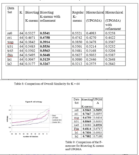
The F-measure results are shown in table 8 – larger is better. UPGMA is the

best, although the two other techniques are often not much worse.

Data Set UPGMA Centroid Cluster

Similarity Similarity

re0 0.5859 0.5028 0.5392

re1 0.6855 0.5963 0.5509

wap 0.6434 0.4977 0.5633

tr31 0.8693 0.7431 0.7989

(11)

Fbis 0.6717 0.6470 0.6233

la1 0.6963 0.4557 0.5977

la2 0.7168 0.4531 0.5817

Table 2: Comparison of the F-measure for Different Clustering Algorithms

The entropy results are shown

in figures 1 - 8. Notice that UPGMA

and IST are the best, with similar

behavior with respect to entropy. CST

does poorly. Figures 1, 5, and 6

indicate that CST does about as well

with respect to entropy as do IST and

UPGMA in the initial phases of

agglomeration, but, at some point,

starts “making mistakes” as to which

clusters to merge, and its performance

diverges from the other schemes from

then on. In the cases represented by

the other figures, this divergence

happens earlier. UPGMA shows

similar behavior, but only when the

number of clusters is very small.

Overall, UPGMA is the best

performing hierarchical technique that

we investigated and we compare it to

K-means and bisecting K-means in

the next section

Comparison of K-means, Bisecting K-means and UPGMA

Here we provide some brief details of how we performed the runs that produced the results

we are about to discuss.

For these experiments we

equalized the number of runs for

bisecting K-means versus customary

K-means. In the event that ITER is

the quantity of trial bisections for

each period of bisecting K-means

and K is the quantity of groups

looked for, then a bisecting K-means

run is identical to log2 (K) * ITER

customary K-means runs. (There are

what might as well be called ITER

K-means keeps running for the entire

arrangement of documents for each

of the log2 (K) levels in the

(12)

bisecting K-means, we set ITER = 5.

We did 10 keeps running of the

bisecting K-means and for each keep

running of the bisecting K-means we

performed log2 (K) * ITER keeps

running of a standard K-means.

Since Hierarchical clustering

produces a similar outcome without

fail, there was no compelling reason

to lead numerous keeps running for

UPGMA.

There is additionally another

issue that must be specified. Both

bisecting K-means and Hierarchical

clustering produce clustering comes

about that can be further "refined" by

utilizing the K-means calculation.

That is, if the centroids of the groups

delivered by these two methods are

utilized as the underlying centroids

for a K-means clustering calculation,

then the K-means calculation will

change these underlying centroids

and rearrange the clusters. The key

question here is whether such

refinement will enhance the nature of

the clusterings created.

We likewise say that

progressive clustering with a

K-means refinement is basically a

Hierarchical K-mean half breed that

is like procedures that other

individuals have attempted.

Specifically, the

Disseminate/Assemble framework

[CKTP92] utilizes Hierarchical

clustering to create "seeds" for a last

K-means stage.

Tables 3 - 5 demonstrate the

entropy aftereffects of these runs,

while tables 6 - 9 demonstrate the

general likeness comes about. Figure

10 additionally indicates entropy

comes about and is simply Figure 1

with the entropy comes about for

bisecting K-means included. Table 8

(13)

between F values for bisecting

K-means and UPGMA. We express the

three principle comes about

concisely.

• Bisecting K-means, with

or without refinement is superior to

anything standard K-means and

UPGMA, with or without

refinement, as a rule. Indeed, even in

situations where different plans are

better, bisecting K-means is just

marginally more terrible.

• Refinement

fundamentally enhances the

execution of UPGMA for both the

general comparability and the

entropy measures.

• Regular K-means, albeit

more terrible than bisecting

K-means, is by and large superior to

anything UPGMA, even after

refinement.

We make a couple brief

remarks on the way that we did

different keeps running of K-means

and bisecting K-means. For bisecting

K-means, this did not enhance the

outcomes much as this calculation

tends to create generally predictable

outcomes. For standard K-means, the

outcomes do change a lot starting

with one run then onto the next. In

this way, one keep running of

customary K-means may create

comes about that are not in the same

class as those delivered by UPGMA,

even without refinement.

In any case, even many keeps

running of means or bisecting

K-means are altogether speedier than a

solitary keep running of a hierarchal

clustering calculation, especially if

the informational collections are

vast. For instance, for the

(14)

3204 documents and 31,472 terms, a

solitary progressive clustering run

takes well in overabundance of a

hour on a cutting edge Pentium

framework. By correlation, a solitary

bisecting K-means rush to discover

32 groups takes not as much as a

moment on a similar machine.

Data

Set K Bisecting Bisecting Regular Hierarchical Hierarchical

K-means

K-means with refinement

K-means (UPGMA) (UPGMA)

with

refinement

re0 16 1.3305 1.1811 1.3839 1.9838 1.4811

re1 16 1.6315 1.7111 1.6896 2.0058 1.7361

wap 16 1.5494 1.5601 1.8557 2.0584 1.8028

tr31 16 0.4713 0.4722 0.5228 0.8107 0.5711

tr45 16 0.6909 0.6927 0.7426 1.1955 0.8665

fbis 16 1.3708 1.4053 1.3198 1.8594 1.3832

la1 16 0.9570 0.9511 1.0710 2.4046 1.2390

(15)

Table 3: Comparison of the Entropy for Different Clustering Algorithms for K = 16

Data

K-means

with

refinement

re0 32 1.0884 1.1085 1.2064 1.5850 1.3969

re1 32 1.4229 1.3148 1.4290 1.5360 1.2138

wap 32 1.3314 1.2482 1.4422 1.7201 1.5252

tr31 32 0.2940 0.3327 0.4281 0.5123 0.4641

tr45 32 0.5676 0.4991 0.5293 0.7312 0.4730

fbis 32 1.1872 1.2060 1.2618 1.4538 1.2841

la1 32 0.8659 0.9149 1.0626 1.5375 1.0111

la2 32 0.8969 0.8463 0.9659 1.3568 0.9623

Data

K-means

with

refinement

re0 64 1.0662 0.9428 0.9664 1.3215 1.1764

re1 64 1.0249 0.9869 1.1177 1.1655 0.9826

wap 64 1.1066 1.0783 1.2807 1.3742 1.2825

tr31 64 0.3182 0.2743 0.3520 0.3985 0.3855

tr45 64 0.4613 0.4199 0.4308 0.4668 0.3913

fbis 64 1.0456 1.0876 1.0504 1.2346 1.1430

la1 64 0.8698 0.8748 1.0084 1.3082 1.0066

(16)

Data

K-means

with

refinement

re0 16 0.4125 0.4137 0.4158 0.3157 0.3784

re1 16 0.3325 0.3341 0.3317 0.2703 0.3084

wap 16 0.2763 0.2771 0.2703 0.2440 0.2533

tr31 16 0.4212 0.4231 0.4204 0.3560 0.3619

tr45 16 0.4182 0.4204 0.4190 0.3561 0.3739

fbis 16 0.4464 0.4496 0.4514 0.3657 0.4189

la1 16 0.2228 0.2244 0.2198 0.1420 0.1995

la2 16 0.2282 0.2299 0.2276 0.1694 0.2019

Table 6: Comparison of the Overall Similarity for K = 16

Data

K-means

with

refinement

re0 32 0.4677 0.4788 0.4778 0.4136 0.4421

re1 32 0.3957 0.4009 0.4009 0.3369 0.3690

wap 32 0.3226 0.3258 0.3235 0.2786 0.2876

tr31 32 0.4802 0.4866 0.4795 0.4373 0.4441

tr45 32 0.4786 0.4827 0.4763 0.4299 0.4382

fbis 32 0.4989 0.5071 0.5110 0.4435 0.4827

la1 32 0.2606 0.2640 0.2596 0.1922 0.2247

(17)

Table 7: Comparison of Overall Similarity for K = 32

(18)

CONCLUSION

This paper introduced the

consequences of a test investigation of

some basic document clustering

procedures. Specifically, we

contrasted the two principle

approaches with document clustering,

agglomerative Hierarchical clustering

and K-means. For K-means we

utilized a standard K-means and a

variation of means, bisecting

K-means. Our outcomes show that the

bisecting K-means procedure is

superior to anything the standard

K-means approach and as great or

superior to anything the Hierarchical

approaches that we tried. All the more

particularly, the bisecting K-means

approach creates altogether better

clustering arrangements reliably as

indicated by the entropy and general

similitude measures of cluster quality.

Besides, bisecting K-means appears to

be reliably to improve at creating

document progressive systems (as

measured by the F measure) than the

best of the Hierarchical methods,

UPGMA. What's more, the run time

of bisecting K-means is exceptionally

appealing when contrasted with that

of agglomerative Hierarchical

clustering procedures - O(n) versus

O(n2).

The reason that our relative

positioning of K-means and

Hierarchical calculations contrasts

from those of different scientists

could be because of many elements.

To begin with we utilized many keeps

running of the customary K-means

calculation. In the event that

methods, for example, UPGMA are

contrasted with a solitary keep

running of K-means, then the

correlation would be a great deal

(19)

procedures. Besides, we utilized

incremental refreshing of centroids,

which likewise enhances K-means.

Obviously, we additionally utilized

the bisecting K-means calculation,

which, as far as anyone is concerned,

has not been already utilized for

document clustering. While there are

numerous agglomerative Hierarchical

strategies that we didn't attempt, we

tried a few different methods which

we didn't report here. The outcomes

were similar– bisecting K-means

executed also or

better then the progressive systems

that we tried. At last, take note of that

Hierarchical clustering with a

K-means refinement is basically a half

breed progressive K-means plot like

other such plans that have been

utilized before [CKPT92]. What's

more, this plan was superior to any of

the Hierarchical procedures that we

attempted, which gives us extra trust

in the generally great execution of

bisecting K-means opposite

progressive methodologies.

We alert that the primary point our

paper is not an announcement that

bisecting K-means is "predominant"

to any conceivable varieties of

or conceivable half breed blends with

K-means. Nonetheless, given the

direct run-time execution of bisecting

K-means and the reliably great nature

of the clusterings that it produces,

bisecting K-means is a fantastic

calculation for clustering a substantial

number of documents.

We contended that agglomerative

Hierarchical clustering does not do

well due to the way of documents,

i.e., closest neighbors of documents

frequently have a place with various

classes. This makes agglomerative

Hierarchical clustering methods

(20)

the progressive plan. Both the

K-means and the bisecting K-K-means

calculations depend on a more

worldwide approach, which viably

sums to taking a gander at the

closeness of focuses in a group

concerning every single other point in

the cluster. This view likewise

clarifies why a K-means refinement

enhances the entropy of a Hierarchical

clustering arrangement.

At long last, we set forward the

possibility that the better execution of

bisecting means versus general

K-means is because of certainty that it

creates moderately consistently

measured clusters rather than groups

of broadly differing sizes.

REFERENCES

[1.] Steinbach, M., Karypis, G., &

Kumar, V. (2000, August). A

comparison of document clustering

techniques. In KDD workshop on

text mining (Vol. 400, No. 1, pp.

525-526).

[2.] Jain, A. K. (2010). Data clustering:

50 years beyond K-means. Pattern

recognition letters, 31(8), 651-666.

[3.] Fung, B. C., Wang, K., & Ester, M.

(2003, May). Hierarchical document

clustering using frequent itemsets. In

Proceedings of the 2003 SIAM

International Conference on Data

Mining (pp. 59-70). Society for

Industrial and Applied Mathematics.

[4.] Jing, L., Ng, M. K., & Huang, J. Z.

(2007). An entropy weighting

k-means algorithm for subspace

clustering of high-dimensional

sparse data. IEEE Transactions on

knowledge and data engineering,

19(8).

[5.] Kanungo, T., Mount, D. M.,

Netanyahu, N. S., Piatko, C. D.,

Silverman, R., & Wu, A. Y. (2002).

An efficient k-means clustering

algorithm: Analysis and

implementation. IEEE transactions

(21)

Available online: https://edupediapublications.org/journals/index.php/IJR/ P a g e | 793 intelligence, 24(7), 881-892.

[6.] Beil, F., Ester, M., & Xu, X. (2002,

July). Frequent term-based text

clustering. In Proceedings of the

eighth ACM SIGKDD international

conference on Knowledge discovery

and data mining (pp. 436-442).

ACM.

[7.] Zhao, Y., & Karypis, G. (2002,

November). Evaluation of

hierarchical clustering algorithms for

document datasets. In Proceedings of

the eleventh international conference

on Information and knowledge

management (pp. 515-524). ACM.

[8.] Zhao, Y., Karypis, G., & Fayyad, U.

(2005). Hierarchical clustering

algorithms for document datasets.

Data mining and knowledge

discovery, 10(2), 141-168.

[9.] Pantel, P., & Lin, D. (2002, August).

Document clustering with

committees. In Proceedings of the

25th annual international ACM

SIGIR conference on Research and

development in information retrieval

(pp. 199-206). ACM.

[10.] Pantel, P., & Lin, D. (2002,

July). Discovering word senses from

text. In Proceedings of the eighth

ACM SIGKDD international

conference on Knowledge discovery

and data mining (pp. 613-619).

ACM.

[11.] Boley, D., Gini, M., Gross,

R., Han, E. H. S., Hastings, K.,

Karypis, G., ... & Moore, J. (1999).

Partitioning-based clustering for web

document categorization. Decision

Support Systems, 27(3), 329-341.

[12.] Hassan-Montero, Y., &

Herrero-Solana, V. (2006, October).

Improving tag-clouds as visual

information retrieval interfaces. In

International conference on

multidisciplinary information

sciences and technologies (pp.

25-28).

[13.] Berkhin, P. (2006). A survey

of clustering data mining techniques.

In Grouping multidimensional data

(pp. 25-71). Springer Berlin

Heidelberg.

[14.] Archetti, F., Campanelli, P.,

Fersini, E., & Messina, E. (2006,

June). A hierarchical document

clustering environment based on the

(22)

Available online: https://edupediapublications.org/journals/index.php/IJR/ P a g e | 794 International Conference on Flexible

Query Answering Systems (pp.

257-269). Springer Berlin Heidelberg.

G Venkanna

Assistant Professor

Netaji Institute of Engineering

& Technology

Syed Thayyab Hussain

Assistant Professor

Netaji Institute of Engineering