Field Division Routing

Volume 2010, Article ID 560797,17pages doi:10.1155/2010/560797

Research Article

Field Division Routing

Milenko Drini´c,

_{Darko Kirovski,}

_{Lin Yuan,}

_{Gang Qu,}

_{and Miodrag Potkonjak}

1_{Microsoft Research, One Microsoft Way, Redmond, WA 98052, USA} 2_{Synopsys, 700 East Middlefield Road, Mountain View, CA 94043, USA} 3_{University of Maryland, 1417 A. V. Williams, College Park, MD 20742, USA}

4_{Computer Science Department, UCLA, Boelter Hall 3532G, Los Angeles, WA 90095, USA} Correspondence should be addressed to Milenko Drini´c,[email protected]

Received 15 December 2009; Revised 15 April 2010; Accepted 17 June 2010

Academic Editor: Athanasios V. Vasilakos

Copyright © 2010 Milenko Drini´c et al. This is an open access article distributed under the Creative Commons Attribution License, which permits unrestricted use, distribution, and reproduction in any medium, provided the original work is properly cited.

Multihop communication objectives and constraints impose a set of challenging requirements that create difficult conditions for simultaneous optimization of features such as scalability and performance. Routing in wireless multihop networks represents a crucial component of the overall network efficacy because it is a lower layer that enables the actual functionality of networks. We have developed field division routing (FDR), a distributed and nonhierarchical routing protocol that aims to coordinated addressing of scalability, topology alternations, latency, throughput, energy efficiency, and local storage requirements. FDR is based upon two optimization mechanisms: a reactive and focused diffusion that collects only network topology information directly required for making localized routing decisions, and a protocol for sharing routing information among neighboring nodes. Routing table initialization and maintenance are scalable in terms of both storage and overhead traffic necessary for building routing tables. FDR provides guaranteed connectivity while providing near-optimal all-node-pairs message delivery. The protocol is also power-efficient to a wide spectrum of topology changes that induce relatively few messages to update routing tables network-wide. We analyzed the new routing protocol both theoretically and using simulation.

1. Introduction

Wireless ad hoc networks (WAHNs) are commonly abstracted as a system of application-specific devices (nodes) with processing, storage, communication, and often sensing capabilities where nodes communicate via radio frequency waves. The communication range is often substantially shorter than the network diameter. Therefore, each node acts as a router and communicates with other nodes via a multi-hop protocol. Routing protocols in WAHNs play an important role as they have ramifications on the key system requirements: (i) scalability, (ii) resilience to topology change, (iii) overall node connectivity, communication (iv) latency (delay) and (v) throughput, (vi) power consumption, and (vii) local storage requirements [1]. The role of routing in WAHNs is to enable primary functionality of a network such as monitoring of objects, detection of different type of events, and data distribution and dissemination with a purpose for actuation on observed events. Due to its

importance, routing in WAHNs has been addressed in numerous proposals that target various subsets of the seven criteria. Nevertheless, due to the complex set of often contradictory requirements, the search for ever improving protocols continues.

Routing decisions in WAHNs are supported either using routing tables that specify the network topology or using a geographic routing criterion for making localized forwarding decisions (seeSection 2). The first class of protocols requires hard-to-scale worldwide routing table updates upon each topology change, while guaranteed message delivery (see

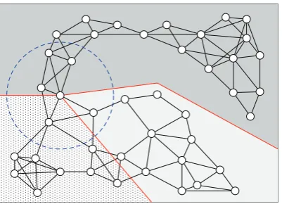
Figure 1) and shortest-path communication are the key challenges for the latter class.

Figure 1: Challenges of multi-hop routing: In a relatively chal-lenging setting with four disjoint communication obstacles, we generated a fully connected network of 200 (illustrated), 500, and 1000 nodes. GPSR [2] succeeded in connecting only 79%, 88.6%, and 90.3%, respectively, node pairs; thus, in a randomly generated traffic model, approximately 10–20% of all traffic is likely not to reach destination in these networks.

topology changes. We aim for this objective and propose a novel, distributed protocol, field division routing (FDR), that targets all of the seven system requirements. In FDR, each node contains all information necessary to distribute messages to any other node in the network; each node derives this information based upon the geographic location of a relatively small subset of nodes, which are located in its vicinity. Each node divides the geographical network field into a tile of zones unique for this node. Traffic to all nodes in one zone is routed via a neighbor uniquely assigned to that zone. If all FDR tables are computed centrally, they enable all-shortest-paths routing in a network with static topology [3]. Here, we explore the more complex but significantly more energy-efficient and scalable approach where each node computes and maintains its own routing table in the presence of an ever-changing network topology.

Under the mild assumption that the network is within a finite field and that each node is aware of its geographic location, we introduce aDiscoveryprotocol that computes a near-optimal shortest-paths routing table for a given node in a relatively message-intensive manner. SinceDiscovery

must be repeated for each node upon every topology change, we reduce the network maintenance overhead by introducing a novel and near-optimal procedure for routing table

Inheritance from neighboring nodes. Next, we propose a distributed protocol for network “initialization” with an objective to reduce the number of nodes that perform

Discovery while computing their routing tables. In order to support a dynamic network topology, that is, arbitrary motion of nodes and obstacles, we introduce algorithms for routing table “updates” that address node movement that is modeled by node appearance and disappearance. The two procedures are based upon the low-cost Inheritance

protocol. Therefore, we believe that FDR addresses the key system requirements (i–vii) simultaneously; it is scalable, establishes provable connectivity, is power efficient because network dynamics initiates few messages to update routing tables, enables near-optimal shortest-path message delivery, and its routing tables are compact.

A shorter version of this paper with the same title has been presented in [4]. Compared to the shorter paper, this paper contains more detailed explanation of the underlying FDR concepts with additional examples for better clarifica-tion. It also contains an extended set of experimental results. Finally, it contains proofs for all the presented theorems, which were omitted in the previous version due to space constraints.

2. Related Routing Protocols

Routing protocols for WAHNs can be categorized as proac-tive, reacproac-tive, or hybrid. Each node that uses a proactive protocol stores sufficient data about the network topology in its routing table. Routing tables are periodically updated such that any time a node needs to send a packet, the forwarding route is already known and can be immediately used [5–8]. Proactive protocols involve high overhead; size of routing tables does not scale well with network growth and routing table updates typically require some form of network flooding. Also, the cost of routing table maintenance rises with increased node mobility. One of the efforts aimed at reduction of network flooding due to change in network topology is Fisheye State Routing, which disseminates infor-mation in such a way that frequent updates are limited to node’s geographical vicinity while the frequency of updates is reduced for nodes at larger distances [9].

In reactive protocols, a node initiates route discovery only when it forwards a packet. Frequently used routes are cached. Reactive protocols are suitable for highly dynamic networks where node mobility renders the cost of proactive protocols prohibitive [10–12]. The topology of WAHNs is closely related to the relative positions of nodes. Geographically assisted protocols exploit this property by making localized decisions on forwarding routes. Greedy Perimeter Stateless Routing (GPSR) [2] reduces the network topology to a planar graph. It forwards messages in the direction of an intended receiver while avoiding areas without forwarding nodes—as a consequence, GPSR cannot guarantee successful message delivery (seeFigure 1). An extension to GPSR deals with realistic connections that often do not correspond to typically assumed unit graph network representations [13]. LAR [14] and CarNet [15] use node locations and a grid to limit the search for new routes. The main drawback of reactive protocols is increased message latency and traffic overhead due to route discovery for each noncached route.

Some of the most popular current research direction for protocols in WAHNs include techniques for identification of connected dominating set for formation of a virtual backbone for dissemination of updating information for routing tables [23–25], predictive cashing strategies [26], new variants of zonal routing [27], and exploration of dynamic addressing techniques [28].

A related class of routing algorithms is clustering-based protocols. In such algorithms, nodes are grouped into clusters such that for each cluster there is an elected node that collects, processes, and forwards data from all the nodes within its cluster to a base station. If compared by a routing criterion, these algorithms are similar to zone routing algorithms. This class of routing algorithms combines network layer with a data layer to achieve flexibility bandwidth and resource allocation, and improved power control. Algorithms from this class are distinguished among each other by the way a cluster is formed and the way a central cluster node is elected. One of the first in this class of algorithms is Low-Energy Adaptive Clustering Hierarchy (LEACH), which changed the premise how an elected node in a cluster has to be fixed [29]. LEACH-C is a centralized version of LEACH where a base station utilizes its knowledge about a network in order to optimize clusters and elected nodes [30]. Power Efficient Gathering in Sensor Information Systems (PEGASISs) enhances collaboration among nodes within a cluster and thus improves network operation life-time [31,32]. Base Station Controlled Dynamic Clustering Protocol (BCDCP) utilizes a high-energy base station to set up clusters and routing paths, perform randomized rotation of cluster heads, and carry out other energy-intensive tasks [33]. Among more recent approaches is Cluster-Chain Routing Protocol (CCRP), which introduces adaptive power adjustment strategy in order to take into account more realistic wireless network connections [34].

FDR is a proactive hybrid non-hierarchical (“flat”) protocol. In addition, FDR is fully distributed; no node needs directions from a centralized location (base station) in order to make routing decisions. At each node, FDR stores and updates only information that is necessary to make routing decisions at that node. Thus, FDR does not store or update the entire network topology for each node, which is required for other “flat” routing protocols. Simultaneously, it provides each node with the ability to forward messages to any part of the network. Size of FDR tables and update cost is comparable to hierarchical protocols, but FDR avoids burdening certain nodes with routing all messages from/to their assigned zones. In addition, FDR is resilient to irregularities of nodes’ communication radius [13, 35,

36]. Since FDR uses network topology to derive routing tables, these irregularities affect only the shape of the routing zones. As a key result, FDR addresses well the key system requirements (i–vii).

3. FDR—Preliminaries

In this section, we introduce a set of assumptions and basic definitions. First, we constrain geographically the considered class of networks to a limited area of arbitrary shape.

We refer to this area as the “network field”. A set of N

nodesN = {n1,. . .,nN}is distributed within the network

field. We assume that each node is aware of its location. This can be achieved either using a global positioning system or a location discovery algorithm [37]. Two nodes can communicate only if the Euclidean distance between them is smaller than their communication range and there are no obstacles to their communication. Communicating nodes are called “neighbors”. For brevity, we adopt that the communication range of all nodes in the network is a constant,r. This assumption is strict, however, the proposed algorithms tolerate variability ofrwithin the network as well as for a single node over longer periods of time.

We model the dynamics of network’s topology using two atomic events: “appearance” and “disappearance” of a node in/from the communication range of another node. Using these two events, we model node motion, creation or destruction of a node within the network field, and communication obstacles in motion. We do not impose any constraints on the frequency of these events, though their frequency may affect adversely the routing efficiency of the system. A node moving fast within the network field may be disconnected from the nodes in the network other than its immediate neighbors, until it reduces speed of motion. We adopt the Random Walk mobility model [38].

From the viewpoint of a single nodeni, the network field is tiled into “routing zones” Zi = {z1i,. . .,ziZi}. Each set of

routing zones is node specific. Each zone inZi_{is a polygon of}

arbitrary shape with one corner positioned atni. Each zone inZi_{is assigned exactly one neighbor toni. We denote|Z}i_|

as the cardinality of the setZi_.

Definition 1(Routing Neighbor). Exactly one neighbor toni

is assigned to each of its routing zones. We define such a neighbor as a routing neighbor.

Each routing zone is defined with up to two “borders”.

Each border is defined using a set of straight chain-connected “border line segments”, whereas each border line segment (abbr., line) connects a pair of “border points”.In the general case, border lines could be represented using polynomials of arbitrary degree. In order to reduce the complexity of calculations, we adopted the border representation with a polynomial of the first degree. A zone is defined using two borders that originate at ni and intersect as a final point the border of the network field. The field border connects borders’ ends to form a single polygon. In a less frequent case, a routing zone does not extend to the border of the network field. (In our experiments, the frequency of occurrence of such cases ranges approximately from 0.0001% to 0.001%.) Such a case can occur in a network with large areas that do not contain any nodes. In such case, a routing zone is described using a single border which starts and ends at

ni. Since this type of a routing zone occurs infrequently, throughout this paper, we refer to routing zones defined using two borders.

FDR supports two fundamental message delivery mech-anisms: location and name based. In case a source node

Figure2: An example of a network field divided into three routing zones for nodes. Each zone is assigned to respective neighbor nodes a,b, andcofs. Routing zones are defined using pointsx1,x2,x3, andx4.

nj, it finds the routing zone that contains nj and sends

the message to the routing neighbor assigned to that zone. Here, we assume that all traffic in the network conforms to this model. FDR can be adjusted to support name-based message delivery as well. Next, the source node must first discover the geographic position of the destination node and then forward the message using the location-based delivery process. There are several simple protocols that can be used to announce the position of a node to the remainder of the network. Detailed analysis of name-based message delivery protocols is beyond the scope of this paper.

An example of a WAHN is shown in Figure 2. We consider the routing zones built from the viewpoint of nodes. Nodesdivides the network field into three routing zones. These zones are assigned to neighboring nodes a,

b, and c. The neighboring node a is assigned to the routing zone described with borders{(s,x1), (x1,x2)}, and {(s,x3)}. The neighboring nodebis assigned to the routing

zone described with borders {(s,x3)} and {(s,x4)}. The

neighboring nodecis assigned to the routing zone described with borders{(s,x4)}and{(s,x1), (x1,x2)}. Full description

of each routing zone includes the border of the network. We assume that each node knows the defining points of the enclosing network field:y1,y2,y3, andy4. Thus, the routing

table for each node contains only information about the tiling of the network field into zones.

4. Routing Table Initialization

In this section, we describe how nodes initialize their routing tables using FDR. During initialization, each node divides the network field into routing zones and assigns a routing neighbor to each routing zone. The construction process relies on several key observations related to network topology and connectivity.

Definition 2 (Essential Node). If the shortest path from a source nodenito a destination nodenjleads exclusively via

one neighbornkofni, thennjis a node essential toni.

s

a1

a2

a3

b1

b2

b3

b4

d2

d3

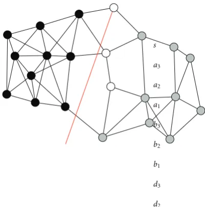
Figure 3: An example of a network used to demonstrate why a network field is divided by essential nodes.

Definition 3(Essential Neighbor). Letnjbe an essential node

to ni. A neighbor nk of ni, which is the first hop on the shortest path from ni to nj, is referred to as an “essential neighbor” ofni.

Consider the example inFigure 3. Nodesis the source. Then, nodes a2 and a3 are essential nodes because the

shortest path to these nodes leads only via nodea1. Similarly,

b2,b3, andb4are essential nodes since the shortest path from

s to any of them leads only via b1. Nodes a1 and b1 are

essential neighbors ofs.

To achieve shortest-path routing, a message from a source node toward any essential node must be routed only via other essential nodes of the source. Consider the nodeb3

in the example inFigure 3. All messages fromstob3haveb1

as their first hop. Note thatb3is not an essential node ofb1

because two shortest paths fromb1tob3exist viab2andb4,

respectively. However, bothb2andb4are essential nodes tos.

We formulate the above statements more formally.

Theorem 4. The shortest path from a source nodestoward any essential node routed via the same neighbor nleads only via nodes that are essential tos. (Proofs of all theorems are included in the appendix.)

Theorem 5. The shortest path from a source nodestoward any nonessential node leads only via nonessential nodes.

4.1. Selection of Routing Neighbors. When a source node is building its FDR table, it has to determine how many zones will divide the network field (|Zi_{|) and select the}

Based onTheorem 4, we know that the shortest path to all essential nodes leads only via essential nodes.

Corollary 6. From Theorem 4, it follows that if there is an essential nodeeat distanceαhops from a source nodes, where α > 2, there exists an essential node at distance 2 fromsvia which the shortest path leads toe.

Corollary 7. From Theorem 5, it follows that if there is a nonessential nodenat distanceβfrom a source nodes, where β >2, then there exists a nonessential node at distance 2 froms via which the shortest path leads ton.

From Corollaries6and7, it follows that a node can deter-mine which of its neighbors are essential and nonessential by observing the network topology at a distance of two hops from itself. In other words, a node can which the necessary of routing zones is necessary to cover the entire network by only observing neighboring network topology at distance of 2 hops from itself. This topology can be easily obtained for each node in a network if each node broadcasts a list of its neighbors.

We describe this process using an example inFigure 3. Nodesbroadcasts a message to its neighbors requesting that they send the list of their neighbors. Nodea1 returns a list

with nodesa2andd2, andb1returns a list with nodesb2,b4,

andd2. Nodesconcludes thata2is only covered by nodea1

and therefore it is essential. Similarly, nodes b2 andb4 are

essential, while node d2 is covered by both neighbors. We

denoted2a don’t-carenode. In this case, both neighbors are

essential. Thus,screates two routing zones with nodesa1and

b1 assigned to each zone. A source node selects all essential

neighbors and a subset of nonessential neighbors as routing neighbors such that all nodes in the network are covered.

Definition 8(Don’t-care Node). A node that can be assigned to either routing zone with preserved shortest path routing is a “don’t-care node”.

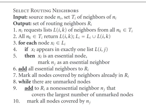
Algorithm 1outlines the algorithm that identifies essen-tial and nonessenessen-tial neighbors and selects routing neigh-bors. The goal of the algorithm presented in Algorithm 1

is to select as few as possible nonessential neighbors that are assigned to routing zones. Since each routing neigh-bor corresponds to one routing zone, by minimizing this number, we heuristically aim at reducing the number of stored borders, that is, the storage requirement, at each node. This problem can be reduced to the constrained minimum sequence covering problem (CMSC), which is NP-hard [39]. CMSC can be defined as follows.

Problem. Constrained minimum sequence covering.

Instance. A finite sequence of symbolsD= {d1,d2,. . .,dn}; a

set of templatesT= {t1,t2,. . .,tk}such that each templateti

is formed by concatenating an arbitrary number of symbols from D; sequence S formed by concatenation of symbols fromDand integerI.

Question. CanSbe covered byIinstances ofTsuch that no two templates overlap andIis minimized.

Select Routing Neighbors

Input:source nodeni, setTiof neighbors ofni

Output:set of routing neighborsRi

1.nirequests listsL(i,k) of neighbors from allnk∈Ti

2. Allnk∈TireturnL(i,k);Li=Li∪L(i,k)

3.for eachnodexl∈Li

4. if xlappears in exactly one listL(i,j)

5. then xlis an essential node,

marknjas an essential neighbor

6.addall essential neighbors toRi

7. Mark all nodes covered by neighbors already inRi

8.whilethere are unmarked nodes

9. addtoRia nonessential neighbornjthat

covers the largest number of unmarked nodes 10. mark all nodes covered bynj

Algorithm 1: Procedure that selects and assigns neighbors to routing zones.

If we consider node to correspond to a symbol, node connectivity to correspond to a concatenation of symbols into a sequence, and a selection of a neighbor that covers certain number of nodes to correspond to a template that covers the corresponding sequence of symbols, our problem is reduced to CMSC. To address this problem, we propose a particularly fast, but greedy heuristic. Note that the heuristic may not return an optimal solution in this context, however, in the next phase of building node’s routing table, shortest-paths routing to all destinations can still be achieved.

4.2. Nodes Sufficient to Build a Border. The geography of a routing zone is dependent upon the positioning of the encompassed essential nodes. In the remainder of this paper, we refer to all nodes covered exclusively by a single routing neighbor as “essential nodes”.Nodes covered by more than one routing neighbor are referred to as “don’t-care nodes”. In both cases, for node nk to “cover” node nj from the perspective of a source node ni means that nk is on the shortest path from ni to nj. If a source node identifies all essential nodes, it can identify all routing zones to achieve shortest-paths routing. Unfortunately, in order to identify all essential nodes, it appears that the source has to flood the network. As this cost is prohibitive, we propose a more effective solution.

In order to build borders between zones, it is not necessary for a source node to have knowledge of the entire network topology. Consider the example network in

Figure 4. Source nodesneeds to build a border between two routing zones assigned to nodesa1andb1(a border line that

originates ins). Let us assume thatshas two lists of nodes: (i)

a2anda3; and (ii)b2andb3. The nodes in the lists represent

nodes that are the closest to the border between zones. They are sufficient to completely describe the border. Nodescan ignore the positions and connections of all other essential nodes on either side of the border while constructing it.

s

a3

a2 a1

b3 b2 b1

d3 d2

Figure4: An example of a network used to demonstrate why it is sufficient to select only a subset of all essential nodes for the process of building borders.

The key idea behind this protocol is to send two messages along each side of the border. The messages carry the hop count from the source and a border side identifier (i.e., coun-terclockwise (CCW) or clockwise (CW)). This information enables nodes along the border to identify if they are essential or “don’t-care” nodes from source’s perspective. Source node

s uses geographical location of routing neighbors pairs to determine which one carries CW and which one CCW type of a message. Note that in cases whenshas only two routing neighbors (such as for nodesinFigure 4), only two borders are created. When creating one border, the first neighbor is on CW side, the second one is on CCW side. When creating the other border, routing neighboring nodes switch roles so the first neighbor is on CCW side, and the second one is on CW side. We demonstrate the protocol using an exemplary network in Figure 4. Source node s identifies thata1 and

b1 are its essential neighbors and sends a message to a1

andb1 requesting a list of essential nodes along each side

of the border. In the message,s states that the border is in the CW direction fora1 and CCW direction for b1 withs

as a reference node. It also states that noded2 is a

“don’t-care” node. Nodea1 identifiesa2 as the closest node to the

border with a hop count of 2, while b1 identifiesb2. They

further request froma2andb2to return a list of nodes along

the border. This request includessas a reference node and respective orientations. Nodesa1andb1informd2that it is

a “don’t-care” node with a hop count of 2;d2announces this

information to all its neighbors. Next, nodeb2identifies and

notifies b3 as the node closest to the border (in the CCW

direction) with a hop count of 3; b3 acknowledges that it

is at the end of the network field and returns a list to b2

that contains nodeb3. Next,b2appends itself to the list and

sends it back to b1, and b1 sends a list containing b2 and

b3 to s. On the other hand,a2 identifies and notifiesd3 as

the one closest to the border (in the CW direction) with a hop count of 3; d3 receives the broadcast message fromd2

thatd2is a “don’t-care” node with a hop count of 2. Next, it

receives the message froma2stating that its hop count from

the source node is 3. Since there exists a path viad2with a

hop count of 3,d3concludes that it is a “don’t-care” node.

Discovery

Input:current nodexi, number of hopsh

Output:list of essential nodesLifromxito

the end of network field 1.ifxiis don’t-care

2. xiannounces it is don’t-care to all its neighbors

3. returnempty Li

4.ifxiis at the end of the network field

5. returnLi=xi

6. Sort neighbors ofxi,{n1,. . .,nk}, into a listNi,

7. the closest node to the border is at the head ofNi

8.for eachneighbor nj∈Ni

9. Li=callDiscovery(nj,h+ 1)

10. ifLi=/ empty

11. prependxitoLi, that is,Li=xiLi

11. returnLi

12.returnempty Li

Algorithm2: Pseudocode for FDR’sdiscoveryprotocol.

It announces this information to all its neighbors. Similar to

b2,a2identifies and notifiesa3as the closest to the border in

the CW direction that is not “don’t-care”. Soon, it receives a list froma3that contains one node,a3;a2 appends itself to

the list, sends it back toa1, anda1 sends the list containing

a2anda3tos. Nodesreceives the list that contains nodesa2

anda3on one side of the border, andb2andb3on the other

side of the border.

The Pseudocode for FDR’s Discoveryprotocol is pre-sented in Algorithm 2. We present only a part of the algorithm initiated by source’s neighbors. This part of the algorithm is recursive. Each node can receive two types of messages from their neighbors: a don’t-care announcement and a request for the list of essential nodes along the border. When a request for the list is received, nodexi first determines if it is a don’t-care node. This can happen ifxi

already received adon’t-careannouncement with smaller or equal hop count, or if it received another request from the opposite side of the border with the same hop count. In such a case,xiannounces to its neighbors that it is a don’t-care node. Otherwise, xi sorts its neighbors such that the closest node to the border is at the head of the sorted list. Since the border is not placed yet,xiuses the reference point and a direction (CCW or CW) to determine the ordering. Then,xirecursively requests the list of essential nodes from its neighbors in the sorted order. The bottom of this recursive procedure is when the end of the network field is reached. Pseudocode in Algorithm 2 is presented in the form of a function that handles the requests for the list of essential nodes along the border. The function returns a list that is empty if a node is adon’t-carenode.

Each node, when added to the network, is informed about its boundary. We do not make any assumptions about the shape of the finite network field. In our tests, we assumed a rectangular field.

Discovery attempts to find all nodes necessary for creation of zones’ borders. Due to the fact that this algorithm is localized, sometimes it can produce borders where shortest path routing is not preserved. We formalize this observation in the following Theorem.

Theorem 9. Discoverycan yield suboptimal results in terms of shortest path routing.

Although Discovery can produce suboptimal results, it is important to note that the connectivity of nodes is preserved. This fact is very important for guarantied message delivery.

Theorem 10. Discoverymaintains node connectivity.

An important property of any routing scheme is its ability to forward messages without cyclic paths. Cyclic paths can result in buffer overflows, excessive energy bill, and dead locks; clearly, they contribute to the overall inefficiency of the network.

Theorem 11. FDR is an acyclic routing scheme.

4.3. Building Borders. The source node initiates the pro-cedure for building borders upon receipt of the two lists of essential nodes (CW and CCW from the border) from the associated pair of routing neighbors. The goal of this procedure is to create a chain of border line segments that separates two routing zones such that node motion is maximally tolerated. This is accomplished by placing the border equidistantly from closest essential nodes in each zone. We describe this procedure using an example in

Figure 5. The source nodesconsiders essential nodesa2,a3,

a4, anda5along one side of the border (CW) andb2,b3, and

b4along the other (CCW). Nodesuses one pointer for both

received lists. By iteratively advancing these pointers,sbuilds the border. The construction process involves the following steps:

(i) Set pointers pCW = a2 and pCCW = b2 to the

corresponding beginning of each list; set the reference pointr= s; compute the initial minimal angleθ= ∠(pCW,r,pCCW) — at firstθ > 0.

(ii) Iteratively advance both pointers and record minimal

θand correspondingpCWandpCCW; repeat untilθ≤

0. This situation occurs after advancingpCWfroma3

toa4.

(iii) Insert the first border pointc1at half distance from

the previous valid pointers a3 and b3 where θ =

∠(a3,r,b3) > 0; set the reference point r = c1;

computeθ; Reset pointerspCW=a3andpCCW=b3.

(iv) Iteratively advance both pointers until ends of both lists are reached, that is,pCW=a5andpCCW=b4.

s

a3

a2

a1

b3

b2

b1

d3

d2

Figure 5: A network example that illustrates the procedure for building borders.

(v) Insert the last border pointc2 at half-distance from

the current pointersa5andb4.

The Pseudocode of this procedure is shown in

Algorithm 3. The procedure does not attempt to insert the minimal number of border points in order to address the (vii) criterion. We have opted for a strategy where a border point is inserted equidistantly between two conflicting pointers. This enables less frequent updates of borders since changes in node positions have the least effect on borders. As most of the borders are composed of only a single border point, the overall increase in the average routing table size is negligible.

BuildBorders

Input:LCCWand LCW—lists of essential nodes,

pCCWandpCW—node pointers, source nodes Output: C—list of border points

1. Set reference pointr=s

2. SetpCCWandpCWto the node closest tosin LCCWandLCW, respectively

3. Last valid pair of pointers{V1,V2} = {pCCW,pCW} 4. Computeθ=∠(pCW,r,pCCW)

5.repeat

6. ifpCCW−r<pCW−radvancepCCW 7. elseadvancepCW

8. Computeθ=∠(pCW,r,pCCW) 9. ifθ <0

10. addpointcitoC,ciis on the lineV1,V2 andci−V1 = ci−V2 11. Place border betweenrandci; setr=ci;

12. θ=∠(V1,r,V2);{pCCW,pCW} = {V1,V2} 13.else ifθ <θ

14. θ=θ;{V1,V2} = {pCCW,pCW} 15.untilbothpCCWandpCWreach ends

ofLCCWandLCW, respectively

Algorithm 3: Pseudocode of the procedure that builds borders between two routing zones of a source node. Operatora−b

returns the Euclidean distance between two pointsaandb.

s

a1 b1

A1₍₅₎

A2₍₁₀₎

(7)

(9)

B1₍₇₎ B2₍₉₎

(5)

Figure6: An example of border placement between two routing zones of a source node based on the routing zones of source’s routing neighbors.

We use the example in Figure 6to describe the Inher-itance protocol. Assume that nodes a1 and b1 are routing

neighbors of a source nodes, both a1 andb1 have already

determined their routing tables via theDiscoveryprotocol. Here, we make an assumption that the routing table for nodescontains an additional information about each border pointci:φi=min{h(s,V1),h(s,V2)}, where functionh(a,b)

returns the hop count from nodea to nodeb andV1 and

V2 are essential nodes that determined the location of ci

Inheritance

Input:CCCW,CCW—lists of border points with the hop count information for each point, source nodes Output:C—list of points for the inherited border 1.for eachborder linel=ci,ci+1inCCCWandCCW 2. insertφi+1−φi−1=P−1 pseudo border points

p0=ci,p1· · ·pP−1,pP=ci+1such that (∀j)pj∈l

andpj+1−pj = pj−pj−1 3.for eachpj

4. compute its hop count estimate:φj

5.for eachborder pointci∈CCCW∪CCW

6. if(∃pj)φj=φiandpjis at opposing border toci

7. addpointttoC, wheretis onci,pjand ci−t = pj−t

Algorithm4: Pseudocode of the procedure that builds a border between routing zones of two adjacent routing neighbors of a source node.

as in step 9 of the Pseudocode in Algorithm 3. Figure 6

illustrates theφ-parameter in parentheses next to the name of a border point. The Inheritanceprotocol executes the following simple steps:

(i) divide each intersecting border line into unit subseg-ments; the unit length equals toci+1−ci/(φi+1−φi),

whereciandci+1are two consecutive border points;

(ii) connect each border point with a mirror point at the other border; a mirror point of a border point is a point with the same estimated hop count at the opposing border line;

(iii) insert points for the new border equidistantly from the connector lines.

These steps assume a uniform probability density func-tion p(x,y) of nodes in the network field. In case p(x,y) is not uniform, a new border point τ is placed such that

τ

cap(x,y)dxdy = cb

τ p(x,y)dxdy, whereca is a point on

one border andcb is its corresponding mirror point. In this case, unit segments are computed similarly, by integrating

p() over the border line. For simplicity of presentation, in this paper we assume thatp() is uniform. Pseudocode for the

Inheritanceprotocol is presented inAlgorithm 4.

At last, we analyze two specific situations. When neigh-bors’ two border zones do not overlap, then Inheritance

uses the procedure BuildBorders from Algorithm 3 to build a new border in between the two nonintersecting borders. The two lists of border points that correspond to the nonintersecting borders are fed as the LCCW and

AsDiscovery, Inheritance can produce zones where shortest path routing is not preserved. This means that some routes will have extra hops in message delivery, which represents an undesirable overhead in communication. It is important to stress that such an overhead should be minimized because in WAHN networks one of the critical resources is typically nodes’ power consumption. Inheri-tancedoes preserve connectivity (guaranteed message deliv-ery) and acyclic routing. We formalize the above observation in the following theorems.

Theorem 12. Inheritance can yield suboptimal results in terms of shortest path routing.

Theorem 13. Inheritancepreserves connectivity.

Theorem 14. Inheritancepreserves acyclic routing.

4.5. Synchronizing the Initialization. We now present an efficient protocol,SynchInit, for distributed and localized network initialization that combines routing table creation via theDiscoveryandInheritanceprotocols. The prereq-uisite condition for applying Inheritance is that routing neighbors of the source node have already initialized their routing tables. We can assess the following optimization goal. Knowing the network topology, select minimal number of nodes whose routing tables are initialized via Discovery, such that remaining nodes in the network can initialize their routing tables viaInheritance.

Consider a network withNnodes. We form a collectionS

ofNsets as follows. For each nodeni, create a set Si= {ni}; then add toSiall nodes for whichniis their routing neighbor. We can restate the optimization goal as the following. Select a subsetBofSsuch that each node belongs to at least one of the selected sets and the cardinality ofB,|B|< K, whereKis a given integer. This problem is equivalent to theminimum set coverproblem, which is NP-hard. This definition of the problem refers to a situation where subsets can be chosen centrally. In our case, the selection process is done in a localized manner. To address the distributed variant of this problem, we propose an effective heuristic with emphasis on protocol simplicity.

The key idea behindSynchInitis to overlay the network field with a regular grid and initialize nodes closest to grid intersections viaDiscovery. The remaining nodes are then initialized via Inheritanceif their prerequisite conditions are satisfied. Next, if there still exist uninitialized nodes, Syn-chInitincreases the grid density and repeats the previous two steps. These two steps can be iterated until all nodes are initialized. Alternatively,SynchInitcan repeat fixed number of iterations and then force all uninitialized nodes to perform

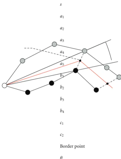
Discovery to complete network initialization. We outline the key steps of SynchInitusing an exemplary network in

Figure 7.

(i) each node considers a virtual regular grid laid over the network field; the grid is the same for all nodes in the network; the shortest distance in the grid equals 2r;

s

a1

a2

a3

a4

a5

b1

b2

b3

b4

c1

c2

Border point

θ

Figure7: An example of an ad hoc wireless network that illustrates the procedure for distributed and localized network initialization.

(ii) nodes closest to intersection points of the grid initialize their routing table via Discovery; such nodes ares,a3,b1,b2,b3, andd2;

(iii) nodes whose routing neighbors have already initial-ized their routing tables useInheritanceto initialize their routing tables; nodes b4 and d3 have routing

neighbors b1 and b3, and a3 and d2, respectively,

that have already initialized routing tables; routing tables can be computed partially, when two angularly adjacent routing neighbors compute their adequate zones, the source can proceed withInheritanceto compute its border;

(iv) double the grid density;

(v) out of all remaining uninitialized nodes, nodesa1and

a2 are the closest to the new grid points; thus, they

initialize their routing tables viaDiscovery.

Remark 15. only nodesb4 andd2 have usedInheritance;

this is a consequence of a denser grid; here, the number of nodes that usedInheritanceis lower than in most practical cases when the network is typically denser.

Pseudocode for this protocol is illustrated inAlgorithm 5. Finally, we evaluate two key trade-offs related to Syn-chInit. First, a denser grid causes more nodes to initiate

Discovery. Then, network initialization converges faster at the expense of sending more messages. Second, we initiateInheritanceQtimes for each iteration ofSynchInit

SynchInit

Input:Noden, comm. ranger, network fieldF Output:Initialized routing table ofn

1. OverlayF using a regular gridG; the shortest distance between two points inGis 2r 2. Find the closest grid pointg

3.repeatRtimes

4. ifnis the closest uninitialized node tog andn−g< r/2

5. returnDiscovery(n) 6. repeatQtimes

7. ifrouting neighbors ofnare initialized 8. returnInheritance(n)

9. Double the grid density 10.returnDiscovery(n)

Algorithm5: Pseudocode for distributed initialization of a routing table. In step 4, if there is a tie in terms of distance, nodes are ordered clockwise north-first to break the tie. In our experiments, we limited R=3 andQ=2.

Inheritancein other nodes. However, this is not feasible if nodes have a mutual relationship of being routing neighbors to each other. Such nodes cannot useInheritanceto build their tables; thus, they wait until the grid density is increased to proceed with their initialization.

5. Support for Network Dynamics

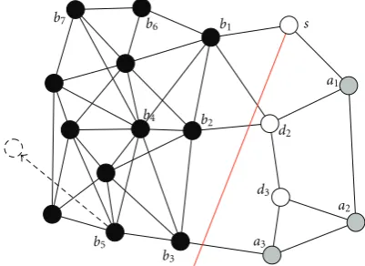
In this section, we propose protocols that can efficiently cope with the management of nodes’ routing tables in the case of a dynamic network topology. We do not bound the space of possible changes in the network. FDR supports introduction of new and failure of existing nodes and/or obstacles to communication in the network field. It also manages the case when both nodes and/or obstacles are in motion. The two atomic events that can model any of these cases are “appearance” and “disappearance” of a node in/from the communication range of another node. We denote these two events as “motion” events. When a motion event occurs, certain nodes may become detached from all but the neighboring nodes in the network because their routing tables are nonexistent or invalid. This condition may last until the node seizes its activity and some or all routing tables of its neighboring nodes are updated. The expectation for this condition is reduced by increasing the communication radiusr of each node. We assume thatr is chosen such that motion events occur relatively infrequently. From the perspective of a specific source node, most of the changes in the network do not have any impact on its routing table. If a motion event occurs far from its routing table’s borders, usually it does not affect source’s routing table. Consider an example shown inFigure 8. If a nodeb5

changes its position as indicated by the dashed arrow, the routing table ofsis not affected. As a network field widens, nodes’ routing zones become larger. For a larger routing zone, it is less likely that an arbitrary motion event in the

b7

b5

b3 b4

b6

b2 b1

a1

a2

a3 d3

d2 s

Figure8: An example of a WAHN that illustrates how node motion does not affect the routing table of a distant node.

network results in an update of its borders. Changes in one part of the network have a smaller expected effect on nodes located far from the place where the motion event occurred. This property enables FDR to be a highly scalable routing scheme when dealing with network dynamics.

The fact that FDR reduces any network topology to rout-ing zones and essential neighbors enables inherent tolerance to small changes to the topology. If two nodes ni and nj

are not essential neighbors to each other, disappearance of

ni from the communication range of any other node in the network does not change the routing table ofnj. If the appearance ofni in the communication range of any node in the network does not establish a new essential neighbor relationship betweenniandnj, it does not affect the routing table of nj. It is important that nodes observe such cases where they do not need to update their tables. This reduces communication overhead. For example, in proactive routing protocols the entire network would have to be flooded with messages about the topology change such that routing tables across the network can be updated. FDR enables situations where network communication is avoided almost entirely even if network topology has changed. We formalize this observation in the following theorem.

Theorem 16. For a given nodeni, appearance or disappear-ance of a neighboring nodenjdoes not affect the routing table ofniif and only ifnjis not a routing neighbor toni. We refer to such a motion event as “unilaterally tolerable ”.

MotionUpdate

Input:Source noden, existing routing tableτ0ofn, nodem appears in its communication range

Output:Routing table ofn

1. Exchange geographic location data withm 2.L=SelectRoutingNeighbors(n) 3.ifm∈L

4. Routing tableτ=Discovery(n) 5. ifτ0=/τ

6. for eachneighborpton

7. ep=PRNG(), send{τ,ep}top

8. returnτ 9. returnτ0 MotionPropagate

Input:Motion evente, source noden, its neighborm, and their routing tablesτ0

nandτm, respectively

Output:Routing table ofn 1. Nodenreceives{τm,e}fromm

2.ifmis a routing neighbor tonand

nhas not yet updated its routing table due toeand τmaffects at least one of the borders inτn0

3. τ1

n=Inheritance(n)

4. ifτ1

n=/τn0thensend{τn1,e}to all neighbors

5. returnτ1 n

6.returnτ0 n

Algorithm6: Pseudocode for routing table update upon a motion event. Function PRNG() returns a pseudorandom number.

When two nodes, n and m, establish communication upon a motion event, each of them executes the MotionUp-dateprocedure outlined inAlgorithm 6. After learning each others’ geographical locations, each node computes its list of routing neighbors as described inAlgorithm 1. Note that

n includes m in its list of routing neighbors only if m is an essential neighbor ton; otherwise,nforces the selection process not to include m. In casemis a routing neighbor, it changes the network topology for n sufficiently so that

n needs to update its table via theDiscoveryprotocol. If there is any change to its routing table borders, n must propagate these changes to its neighbors. Thus, nsends its routing table to all its neighbors as well as a random number

ep distinct for each neighbor p. The purpose of ep is to force the propagation within the network in the opposite direction from n. A random number of sufficiently high entropy should be distinct for this motion event with high likelihood and can be used as its identifier.

A nodenthat receives the propagation packet from its neighbor m executes theMotionPropagate procedure. It ignores the package if mis not its routing neighbor or if the received routing table actually does no affect any of the borders in the existing routing table of n. Otherwise, it recomputes its routing table based on the Inheritance

protocol. Note that only borders affected by the propagation package are recomputed. If there are any changes to the borders of the routing table of n, noden must propagate these changes to its neighbors. The propagation package sent bynincludes the identifier of the original motion event.

s

a1

b1

A1₍₅₎

A2₍₁₀₎

(7)

(9)

B1₍₇₎

B2₍₉₎

(5)

Figure 9: An example of a motion event changing profoundly the network topology and triggering theDiscoveryprotocol for routing table updates.

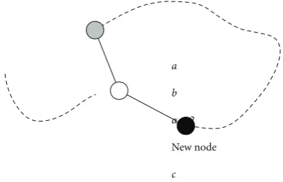
A motion event that triggers propagation is illustrated in

Figure 9. A path of lengthαhops connects nodesa andb, whereα >2. A new nodecestablishes a path betweenaand

b equal to two hops. Thus, botha andbare new essential neighbors toc. Since routing tables ofaandbare affected by the appearance ofc, nodecinitiatesDiscoveryat all three involved nodes.

The main property of the updating protocols is that

Discoveryis performed only by the nodes directly affected by the motion event. In case there are any changes to the routing tables, they are propagated using the localized

Inheritance protocol. In addition, the propagation typi-cally occurs in the immediate neighborhood of the motion event. Only events that profoundly change the topology of the network (e.g., establish a ring as in Figure 9) initiate network-wide propagation. The expectation is that motion events in dense networks should trigger routing table updates significantly less frequently than in sparser networks. Overly sparse networks should experience common wide-spread propagation, a mere necessity for maintaining network’s fragile connectivity. Finally, protocols MotionUpdateand

MotionPropagate preserve the network connectivity and establish acyclic routing. For brevity, we do not present these claims formally in this version of the paper.

to preserve as much as possible of the borders from the existing routing table. This objective minimizes the number of neighbors that propagate their routing table changes.

6. Experimental Results

In order to evaluate the performance of the generic FDR platform, we conducted several experiments. We have compared our approach with GPSR, as a state-of-the-art reactive protocol. We opted for comparison with GPSR because it provides similar support for network dynamics as FDR although its routing algorithm differs significantly. Comparison with proactive or hybrid routing protocols could be done only in one of the performance dimensions because their optimization goals are different from FDR’s so they lack full support for network dynamics and/or they do not offer same routing convenience for each node. We have built a custom simulator for our FDR algorithm and we have implemented GPSR algorithm as it is described in [2].

First, we evaluated if all nodes are reachable. We have established a network with obstacles as shown inFigure 1. More specifically, we created a network field with four obstacles in a realistic setting, that is, a skewed distribution of nodes’ placement in the field. Then, we randomly generated three network instances with 200, 500, and 1000 nodes and measured the percentage of messages that reached destination for each node-to-node coupling in case GPSR was used as a routing mechanism. Only 79%, 88.6%, and 90.3% of messages, respectively, were delivered, while the remainder had to terminate their path search due to exceeded TTL. Most applications that require reliability pose a strong demand for alternate routing mechanisms that guarantee delivery. In addition, name-based messaging in WAHNs (see

Section 3) is particularly prone to failed message deliveries as efficient name-based services commonly require reliable communication.

Figures 10(a) and 10(b) illustrates histograms of path lengths for all pairs of nodes for two randomly generated networks of{N,r} = {200, 0.13},{400, 0.088}. Rangerwas chosen so that the expected number of neighbors for each node is approximately the same regardless of the number of nodes in a network; we aimed at networks of similar density and different area coverage. The benchmark for our measurements was the result of the Dijkstra all-shortest-path algorithm with unit weight for each connection between nodes. We defined routing overhead as an additional number of hops necessary for a message delivery compared to the result given by the Dijkstra algorithm. We measured the results of FDR computed via both the Discovery and

SynchInitprotocols. Also, we computed path lengths using the GPSR protocol excluding connections that were not established. In Figure’s legend we recorded the mean path length across all (in case of GPSR feasible) paths. One can observe that Discoveryfound shortest paths in nearly all cases (overhead of less than 1% and 2.5%) andSynchInit

produced overhead of 5.8% and 8.4% compared to GPSR’s overhead of 9% and 23% (with all infeasible paths excluded) for the network instances of 200 and 400 nodes, respectively.

Figure 10(c) illustrates the number of messages, M, exchanged among all nodes during network initialization. This is the entire initialization cost in FDR. Considered networks are itemized in the caption of Figure 10. Two different datasets are plotted, M for initialization via Dis-covery only and viaSynchInitas described in Section 4. In almost all cases, we recorded improvement in traffic that was nearly constant within 20–25%. For denser networks, this improvement increased, for example, in our experiments we recorded the largest improvement in excess of 60% for

{N,r} = {1000, 0.13}. Note that the number of messages is

comparable to network “flooding;” however, FDR has several important improvements with respect to other “flooding” schemes. First, in FDR M ∼ O(N√N) versus O(N2₎

for true “flooding.” Next, individual nodes do not have to compute the shortest paths upon learning network’s topology, that is, routing tables are computed in a distributed fashion. This greatly reduces the complexity and memory requirement of individual nodes. In addition, FDR’s routing tables require nearly minimal storage which scales well with network size [3]. Finally, FDR supports mobility mostly via the Inheritance primitive which greatly reduces traffic for routing tables’ maintenance once connectivity is established viaSynchInit.

We simulated a large number of motion events. We recorded the trail of messages sent throughout a network in order to propagate information about changes in network topology. We used a uniform distribution to determine a direction of each motion event. We used an exponentially decreasing distribution function to determine the length of each move with the maximum of 3 node communication ranges. For each network type, we simulated 25 000 motion events over 5 different network instances. Each motion event can affect a routing table of a number of nodes, and one or more routing borders within each table. The average number of modified tables ranges from 12.3 for networks with

{N,r} = {200, 0.130}to 17.8 for{N,r} = {1000, 0.060}.

An example of a complete probability distribution is shown inFigure 11.

The likelihood of a node launching the Discovery

protocol due to a motion event ranges from 45% for networks with 200 nodes to 10% for networks with 1000 nodes. An example of such probability distribution is shown inFigure 12.Figure 13presents the overall improvement of the cost (expressed in terms of the number of the exchanged messages necessary for a network update) that is the result of a use of the combination of Discovery andInheritance

protocols, compared to the incurred cost if only the Dis-coveryprotocol is used. The combination of the protocols significantly reduces communication requirements, while maintaining the property thatalltables have updated routes toward all nodes in the network.

7. Conclusion

0 5 10 15 20 25 30 10−4

10−3 10−2 10−1

Path length

P

robabilit

y

o

f

o

ccur

re

nc

e

All-shortest paths (meanL)=5.84

GPSR (meanL)=6.64

NetworkN=200,r=0.13

Discovery(meanL)=5.89 Synchinit(meanL)=6.18

(a)

0 10 20 30 40 50 60 70 80

Path length

P

robabilit

y

o

f

o

cc

ur

re

nc

e

All-shortest paths (meanL)=8.77 10−6

10−5 10−4 10−3 10−2

10−1 NetworkN=400,r=0.088

GPSR (meanL)=10.76 Discovery(meanL)=8.99 Synchinit(meanL)=9.51

(b)

200 400 600 800 1000

0 1 2 3 4 5 6 7 ×105

Number of nodesN

N

u

mber

of

messages

dur

ing

initialization

FullDiscovery Synchinit

Synchinitversus fullDiscovery

(c)

Figure10: Probability distribution for path length in a randomly generated networkN =200,r = 0.13 (a) andN = 400,r =0.088 (b) in a unit-square field. Number of messages sent during initialization usingDiscoveryonly and usingSynchInitfor three network instances for each of the following network types:{N,r} = {200, 0.13},{400, 0.088},{600, 0.071},{800, 0.061},{1000, 0.06}. We selected the communication rangerfor each network so that the expected number of neighbors for each node is approximately equivalent.

due to periodicSynchInitsto optimize path lengths can be negligible in WAHNs where nodes exchange large amounts of data (e.g., audio/video, sensor data) and motion events happen infrequently. Compared to other proactive schemes, FDR offers support for node motion at low cost in overhead traffic and requires low computational resources for nodes. This can be particularly applicable to networks of sensors.

s

a1

a2

a3

b1

b2

b3

b4

d2

d3

Figure 11: Probability distribution of the number of tables and borders affected by motion events for the network type{N,r} = {600, 0.071}.

0 10 20 30 40 50 60 70 80

10−3 10−2 10−1

Instances

P

robabilt

y

of

oc

cur

re

nc

e

Discovery Inheritance

NetworkN=800,r=0.061

Figure12: Probability distribution ofDiscoveryprotocol versus Inheritanceprotocol induced by motion events for the network type{N,r} = {800, 0.061}.

than smaller number of hops. In our simulations, we have neglected a possibility of noisy communication [40], need for message retransmission, dropped connections [34], and so forth. These realistic scenarios can certainly affect a routing protocol. FDR is equipped with mechanisms to handle all of the above issues, whose exploration and the effect on FDR’s performance we leave for future work. Other possible future directions are enhancements in FDR’s border building algorithm where a node could cache already explored lists of nodes that are necessary to build borders; congestion avoidance during message routing; balancing of power utilization for improved network lifetime.

b7

b5

b3

b4

b6

b2

b1

a1

a2

a3

d3

d2

s

Figure 13: Comparison between a system using only the Dis-coveryprotocol and a system that combines theDiscoveryand Inheritanceprotocols.

1 2 3 4

5

2 3 4

s a1

a5

6(5)

r b1

r r

r

r/2 r/2 r/2 r/25(4)r/26(5)r/2

1 2 3 4

z y x

Figure14: An example of a network that illustrates when Discov-eryyields a suboptimal result. Numbers next to nodes represent the hop count from the source nodes. For nodes that have suboptimal hop counts computed by the procedure, optimal hop counts are given in parentheses.

Appendix

Proof ofTheorem 4(by contradiction). Assume that there exists an essential node e at distance α from the source nodes. Next, assume that there exists a nonessential node

lat distanceα−1 fromsthat is connected toe. Sincelis nonessential, there exist multiple neighbors ofs via which

a

b

α >2

New node

c

Figure 15: An example of a network used to prove that FDR is acyclic.

Proof ofTheorem 5.For each nonessential node nj, there exist multiple neighbors of s that can be a first hop on the shortest path. If we remove all these neighbors except one, all nonessential nodes become essential via the unremoved neighbor. Lets denote all nonessential nodes converted to essential nodes via this step aspseudoessential. We can now directly apply Theorem 4 to prove that the shortest path toward anypseudoessentialnode leads via other

pseudoessentialnodes.

Proof ofTheorem 9(by example). Consider an example of a network shown in Figure 14. The source node identifies two routing zones and initiates the process of discovering essential nodes along the border. The numbers inFigure 14

next to each node indicate the length of the shortest path froms, whiler indicates node’s communication range. The following conditions in this example lead to incorrectly calculating the hop count fromstox.

(i) Nodea5has hop count of 5 froms.

(ii) The procedure discovers the subset of essential nodes along the border and calculates the hop count of 6 fromstoy.

(iii) Node z is sufficiently far from the border so the procedure never considers it, and the hop count of 4 fromstozis not calculated.

The calculated shortest path hop count fromstoxis 6 (via

a5) while the correct hop count is 5 (viaz). The procedure

then incorrectly placesxin the same routing zone asA5.

Proof ofTheorem 10.The necessary condition forDiscovery

to yield suboptimal solution is that there exist two paths from a source node to an incorrectly classified node. Even if a node is incorrectly placed into another routing zone, there still exists a routing path from the source node to that node. Thus, a node cannot be disconnected.

Proof ofTheorem 11.We consider two complementary cases; FDR’s routing tables produce an all-shortest-paths routing; and there exist paths that are suboptimal in terms of the length of routing paths. In the former case, each message delivery between two neighboring nodes reduces the distance

to the destination node by one hop because of the shortest path routing. Thus, a source node or any intermediate node on the message path cannot be encountered twice, that is, the routing is acyclic.

In the latter case, we assume that cyclic forwarding of a message has occurred and consider two possible scenarios: (i) there exists a pair of neighboring nodes ni,ni+1 on the

forwarding path such that whennisends a message toni+1,

ni+1returns the message toni, and (ii) a message returns to a

sender via a unique set of nodes (following a cyclic route). For case (i), consider a pair of neighboring nodesniand

ni+1. Let us assume that there exists a nodex at a distance

of two hops fromni which is a neighbor ofni+1. Also, lets

assume that ni routes its messages to x via ni+1. In order

forni+1to return message directed toxback toni, it has to

havenias a first hop towardxin its routing table. However, by the initial assumptionx is a neighbor ofni+1 so all the

messages fromni+1 toxare sent via their direct link. Since

the procedure for selecting routing neighbors (Algorithm 1) considers nodes at distance of two hops, nodesni andni+1

cannot have each other selected as first hops toward the same node. Hence, a node cannot return a message directly to the sender.

For case (ii), we consider a general case illustrated using

Figure 15, when FDR does not follow the shortest path routing and shows that a cyclic routes cannot occur. Dashed lines inFigure 15indicate that there exists a path between two nodes. The label on each dashed line represents the path length. We also use this label as a name for the path. Assume that the shortest path distance from a sourcesto a destinationdisα+ 1 +βhops. Also, assume that there exists another path between nodesaanddwhose length isγand

β < γ. At the same time, assume thatβ < δ+θ < γso node

xmisclassifiesdto be routed via its neighborbinstead ofa. Consider a message forwarded fromstod. Afterαhops, the message arrives at nodex, which forwards it towarddviab. The only way for this message to enter a cycle is that at node

z, it is forwarded back on the path withκhops toward node

c. Whenzbuilds its FDR table, it considers paths of length

θtowarddand pathsκ+ 2 +δ+θorκ+ 2 +γ(latter two are cyclic viac). Nodezdoes not consider the path of length

κ+ 2 +βsince that path has to pass viax, andx does not consider pathβas viable since it is farther from the border than pathγ. Sinceκ+2+δ+θ > θ < κ+2+γ,zalways chooses the pathθfor forwarding. This implies that a path cannot be cyclic. Note that we did not make any assumptions on path lengths except for the conditions necessary to misclassifydin the routing table ofx.

Proof ofTheorem 12(by example). Consider an example of a network shown inFigure 16. Nodesinherits routing tables from nodes a1 and b1. It places a new border such that

nodesa2anda3 are routed viaa1, whileb2,b3, anda4 are

routed viab1. Consequently, the routing path from stoa4

increased from the minimal four hops to five hops, which is suboptimal.