Utility Guided Pattern Mining

(1)

Abstract

JAGANNATH, SANDHYA. Utility Guided Pattern Mining (Under the direction of Dr. Jon Doyle).

This work is an initial exploration of the use of the decision-theoretic concept of utility

to guide pattern mining. We present the use of utility functions as against thresholds and

constraints as the mechanism to express user preferences and formulate several pattern

mining problems that use utility functions. Utility guided pattern mining provides the twin

benefits of capturing user preferences precisely using utility functions and of expressing

user focus by choosing an appropriate utility guided pattern mining problem. It addresses

the drawbacks of threshold guided pattern mining, the specification of threshold and the

assumption of a fixed level of interest. We examine the problem of mining patterns with

the best utility values in detail. We examine monotonicity properties of utility functions and

the composition of utility functions from sub-utility functions as mechanisms to prune the

search space. We also present a top-down approach for generating projected databases from

(2)

UTILITY GUIDED PATTERN MINING

BY

SANDHYA JAGANNATH

A THESIS SUBMITTED TO THE GRADUATE FACULTY OF NORTH CAROLINA STATE UNIVERSITY

IN PARTIAL FULFILLMENT OF THE REQUIREMENTS FOR THE DEGREE OF

MASTER OF SCIENCE

DEPARTMENT OF COMPUTER SCIENCE

RALEIGH

NOVEMBER 2003

APPROVED BY:

DR. PETER R.WURMAN DR. PENG NING

DR. JONDOYLE

(3)

Biography

Sandhya Jagannath was born on October 8th, 1979 in Sakleshpur, India. She received

her Bachelors Degree in Computer Science from Karnataka Regional Engineering College,

Surathkal, India, in the summer of 2001. She has been a Masters student at the North

(4)

List of Tables

1.1 A sample catalog with prices of items . . . 7 1.2 A sample transaction Database, TID denotes the transaction identification

number . . . 7

(7)

List of Figures

5.1 FP-Tree for the transaction database in Table 1.2 . . . 29 5.2 FP-Tree for the projected database in Table 4.1 . . . 29 5.3 Merge of null FP-Tree and tree under(a:2;b:2;d:2;f :2)in Figure 5.1 35

5.4 Merge of tree in Figure 5.3 and tree under(b:2;e :2;f :2)inFigure5:1 . 36

5.5 Thea-projected database cut out of the FP-Tree in Fig 5.1 . . . 39

(8)

Chapter 1 Introduction and Motivation

1.1 Introduction

Frequent Pattern Mining Frequent pattern mining is the mining of patterns that occur frequently in a dataset. It is an important problem in data mining. In addition to frequent

patterns themselves being of interest, frequent pattern mining also plays an essential role

in several data mining problems, such as mining of association rules [2], correlations [6]

and sequential patterns [4].

The frequent pattern mining problem can be described informally as follows. A set of

items is chosen from the domain of interest and is called a catalog. An itemset is a subset

of items from the catalog. The dataset to be mined is a database of transactions, where each

transaction contains an itemset. For example, in the market-basket scenario, the catalog is

the set of all items sold at a store. A transaction contains the set of items bought in one visit

to the store. The transaction database is a set of such transactions.

The support of an itemset is the number of times it occurs in the transaction database. A

support threshold is specified and an itemset is said to be frequent if its support exceeds this

(9)

database that have a support greater than the specified support threshold.

Frequent pattern mining was introduced in [2] as a sub-problem of association rule

mining. This paper presented the division of the association rule mining problem into two

sub-problems, frequent pattern mining and rule generation. Frequent patterns were first

mined from the transaction database and association rules then generated from them. The

complexity of mining the dataset was isolated into the frequent pattern mining step. Since

then much research has gone into increasing the speed and efficiency of this step [9].

Mining Interesting Rules Minimum support guided frequent pattern mining produces large numbers of frequent patterns and consequently a large number of association rules.

Mechanisms to filter out uninteresting rules and generate interesting association rules were

proposed in [10]. Templates were used to allow users to specify items whose presence

made rules interesting and those whose presence made rules uninteresting. Item constraints

were used during the generation of rules after frequent pattern mining.

Constrained Frequent Pattern Mining In constrained frequent pattern mining, con-straints are expressed over properties of items and itemsets. These concon-straints take the form

of requiring the presence or absence of items in frequent patterns or of thresholds on the

values of attributes of items or itemsets that every mined frequent pattern must meet.

Con-straints are integrated into the frequent pattern mining algorithm rather than being used as a

filtering mechanism during or after generation of association rules from frequent patterns.

The selectivity of constraints is used to reduce the number of frequent patterns mined,

making frequent pattern mining and rule generation more efficient. Several constraints

were integrated into frequent pattern mining, including item constraints [16], minimum

(10)

[8], [14]. [16] presents the use of item constraints in frequent pattern mining. Constraints

are specified as boolean expressions over the presence or absence of items or taxonomies

of items. Only frequent patterns satisfying the specified item constraints are mined. Ng et

al in [12] introduce constraints that can be expressed over the domain and class of items, as

also over values and aggregates of item and itemset attributes. The authors also introduce

classification of constraints by properties such as anti-monotonicity and succinctness and

used them to prune itemsets while mining. Such constraints with the property of

convert-ibility are introduced in [14]. Constraint-based mining of correlations, by exploration of

anti-monotonicity, succinctness and monotonicity is studied in [8].

Constrained frequent pattern mining has the following advantages over frequent pattern

mining:

Selectivity of constraints can be exploited to make the pattern mining process

faster and more efficient.

Users can focus mining on the broad phenomena they have in mind [12].

1.2 Motivation

Although constrained frequent pattern mining offers two major advantages over frequent

pattern mining, both suffer the following disadvantages:

Constraints are typically specified as thresholds over values of attributes of

items or itemsets. This poses several problems. It is not clear how a threshold

is to be chosen. A user may guess a threshold and may have to adjust the

threshold if too many or too few itemsets are returned as described in [12].

Constraint pattern mining presupposes a fixed level of interest on the part of

(11)

that do not meet the constraint are not. However, not all patterns returned may

be of equal interest to the user. The user may have preference for one pattern

over another, but there is no way to capture this preference. For example,

amongst all the itemsets that meet a price threshold, the user may prefer the

more expensive ones to the less expensive ones. Such a preference cannot be

captured in the threshold guided setting.

In order to capture user preferences precisely, we examine the use of the decision

the-oretic concept of utility to guide pattern mining. We present the use of utility functions

as against thresholds and constraints as the mechanism to capture user preferences. The

use of utility functions to express user preferences permits several pattern mining problems

to be formulated. We examine one such problem in detail. This work is thus an initial

exploration of the use of the decision theoretic concept of utility in pattern mining.

Decision Theory and Utility Decision theory deals with the making of decisions. A decision consists of choosing an action from amongst alternatives. The set of all

possi-ble actions and outcomes are enumerated. Probability measures are used to indicate the

likelihood of each possible outcome for each possible action.

The decision maker has preferences over outcomes. Given two outcomes A and B,

A B denotes thatB is preferred overA. A B denotes thatAis preferred overB and

AB denotes that bothAandBare equally desirable or equally undesirable.

A utility function is a measure of outcome value. It assigns a numeric value called

utility to each outcome, called the outcome’s utility. A utility function thus ranks outcomes

according to the preferences of the decision maker. If the decision maker prefers outcome

Aover outcomeB, that is,AB, then utility ofAis greater than the utility ofB.

(12)

weighted by their probability of occurrence fora.

A rational action is the one which maximizes expected utility [7].

In this work, the concept of expected utility is not used. Instead, a simplified concept of

utility is used where each action is associated with an outcome and a rational action is the

one which maximizes utility or leads to the outcome preferred most by the decision maker.

Utility Guided Pattern Mining The decision theoretic concept of utility is applied to pattern mining as follows. The user’s preferences over itemsets are captured by a utility

function. The utility function is a measure of the value of itemset to the miner. It assigns a

numeric utility value to each itemset, such that when a miner prefers an itemsetAover an

itemsetB, the utility of the itemsetAis greater than that of itemsetB. The utility function

thus ranks itemsets according to user preferences. Several interesting data mining problems

that use utility functions can be formulated. Utility guided pattern mining consists of using

utility functions to guide pattern mining.

Utility guided pattern mining addresses the problems with frequent and constrained

frequent pattern mining as follows:

Rather than specify thresholds, the user can describe the interestingness of

itemsets by constructing an appropriate utility function. Utility functions allow

expression of interestingness directly. For instance, the utility of an itemset

can be expressed as a function of its attributes. The utility function imposes

an ordering over itemsets and an appropriate pattern mining problem can be

chosen to select itemsets of interest to the user.

Utility functions allow user preferences to be captured precisely. An itemset

(13)

1.3 Examples

The market basket scenario was referred to in section 1.1, when introducing the concept of

frequent pattern mining.

In this section, we present and discuss the market basket scenario in detail. We use it

as an aid to present examples of utility functions and utility guided pattern mining. This

scenario will also be used throughout this work for explaining concepts and for presenting

examples.

The market basket scenario consists of a store that sells some products and buyers that

buy them at the store.

Let the catalog of items sold at a store beC =fa;b;c;d;e;f;g;h;i;jg. The items have

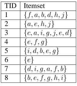
prices as presented in Table 1.1. A transaction database,Dis presented in Table 1.2. Each

transaction in the transaction database contains the set of items bought in one visit to the

store by a customer.

Examples of Utility Functions

1. Let the utility of an itemset be defined as its support in the transaction database. The

utility of the itemsetfa;jgis3.

Some interesting pattern mining problems using this utility function are mining the

most frequent patterns of each length and mining the most frequent patterns from the

transaction database.

The frequent pattern mining problem can be formulated as a utility guided pattern

mining problem two ways. A binary utility function may be used, that assigns a

utility of one to itemsets with support greater than or equal to the minimum support

(14)

Item Price

a 3

b 2

c 6

d 4

e 2

f 1

g 2

h 1

i 1

j 1

Table 1.1: A sample catalog with prices of items

TID Itemset

1 ff;a;b;d;h;jg

2 fa;e;h;jg

3 fc;a;i;g;j;e;dg

4 fe;f;gg

5 fi;d;b;e;gg

6 feg

7 fd;i;g;a;f;bg

8 fb;e;f;g;h;ig

Table 1.2: A sample transaction Database, TID denotes the transaction identification

(15)

is set at5, then the itemsetsfegandfgghave a utility of one and all others have a

utility zero.

The utility of an itemset can also be defined as its support and all itemsets with utility

greater than a specified utility threshold can be mined. This leads to the expression

that all itemsets with support above the threshold are interesting and an itemset with

greater support is more interesting than another one with lesser support. If the support

threshold is set at2, then both itemsetsfa;jgandfe;ggare interesting, butfe;ggis

more interesting thanfa;jg.

2. In the market basket scenario, an interesting problem is mining itemsets that have

fetched the highest revenues over a period of time. The utility of the itemset here is

its revenue, described as the product of the price of the itemset and its support. For

instance the utility of itemsetfe;f;ggis25, that is10.

3. Suppose a supermarket chain sells its own line of cheaper products alongside other

well known and possibly more expensive brands. If a transaction contains a larger

share of brand name products as against products from the supermarket’s line, it

could signal that the user prefers brand name products. A product from the

super-market’s line in this transaction would indicate that the product fulfills a need that

the brand name products aren’t fulfilling. On similar lines, a brand name product in

a transaction with a majority of the supermarket’s line of products could signal that

there is a need that the supermarket line is not fulfilling yet. Utility functions can be

(16)

Chapter 2 Terminology and Definitions

The previous section presented several examples that use utility functions in pattern mining.

In this section, the terms and notations that will be used hereafter in this work to discuss

utility guided pattern mining, are defined formally. Definitions and terms are explained

using the market basket scenario from Section 1.3.

LetC be the catalog of all possible items. It is defined as a finite set of all items from a

domain of interest. In the market basket scenario in Section 1.3, the catalog is the set of all

products sold by the store, that is,C =fa;b;c;d;e;f;g;h;i;jg.

LetN =jCjdenote the number of items inC. In our example,N =10.

Anitemset is defined as a subset ofC. Itemsets are sets and therefore have no

repeti-tions of items.

Examples of itemsets arefa;b;jgandfd;b;jg.

LetI(C), abbreviated asI,I =2 C

, be the set of all itemsets fromC.

I n

(C), abbreviated asI

n, denotes the set of all itemsets of size

nfromI.

LetLbe a set of transaction identifiers.

A transactionis a two-tuple, (TID;I), where TID 2 L and I 2 I. If t denotes a

(17)

Consider the transaction database,D, presented in table 1.2. This transaction database,

D, has eight transactions, each of which is identified uniquely inD by itsTID. An

ex-ample of a transaction is t = (3;fc;a;i;g;j;e;dg). Here t:tid = 3 and t:itemset =

fc;a;i;g;j;e;dg.

T(L;C), abbreviated asT,T =LI, is defined as the set of all possible transactions.

A set of transactions,D T, is called atransactiondatabaseiffDis functional in

L, that is, ift2D, thent:tiduniquely identifiestwithinDin the sense that ift 0

2Dand

t:tid=t 0

:tid, thent=t 0

.

D(T), abbreviatedD, denotes the set of all possible transaction databases overT.

A transactiontcontains an itemsetXifX t:itemset. The transactiont=(3;fc;a;i;g;j;e;dg)

contains the itemsetfd;g;eg.

An itemsetXoccurs in a transaction databaseDif somet 2DcontainsX.

For a transaction databaseD,I(D)denotes the set of all itemsets that occur inD.

For a transaction databaseD,I n

(D)denotes the set of all itemsets of sizenfromI(D).

A utility function is defined as a real valued function, U : (I D) ! R. U(I;D)

denotes the utility or worth of the itemsetIappearing in the transaction databaseD.

In Example 2 in Section 1.3, the utility functionU is defined asU(I;D)=price(I)

support(I;D), where the price of an itemset is the sum of the prices of the items in it.

For example, let I be the itemset fb;dg. Let the prices of items b and d be $2 and $4

respectively. The support of the itemset, support(I;D) =3. The utility of the itemsetI,

(18)

Chapter 3 Formulation Of Pattern Mining Problems Using

Utility Functions

We introduced and formalized the use of utility functions in pattern mining in Chapters 1

and 2. In this Chapter, we discuss several pattern mining problems that use utility functions.

The problems are listed and discussed as follows.

1. Given a utility function, the basic mathematical problem is to evaluate the utility of

every itemset that occurs in the transaction database. This amounts to ranking all the

itemsets that occur in the transaction database by utility. This is the basic problem

only in the mathematical sense, a complete ranking over all itemsets is not typically

computed in practice. So it will not typically be a practical problem.

This problem is stated formally as follows:

Given a utility functionU and a transaction databaseD, for each itemsetI 2 I(D),

calculateU(I;D).

or

(19)

their utility.

2. Mining a specified number of itemsets from a transaction database, that have the best

utility values w.r.t a utility function is an important pattern mining problem. This

allows the user to specify both the number,N, of itemsets he/she wants returned and

the utility ordering over them. N itemsets, from amongst the itemsets that occur in

the transaction databaseD, with the best utility values are returned. This problem is

stated formally as follows:

Given a utility function U, a transaction database D and an integerN > 0, return

N itemsets from I(D) such that for anyI;I 0

2 I(D), ifI is amongst the N best

returned andI 0

is not, thenU(I;D)U(I 0

;D).

Thus, itemsets inI(D)with the best utility values are returned. That is, any itemset

amongst theN itemsets returned has utility equal to or better than the utility of any

item that is not returned.

The product recommendation problem, Example 2, discussed in Section 1.2

recom-mendsN itemsets with the best utility values to the buyer.

3. Mining theN best itemsets can be restricted to itemsets of a certain size. The user

specifies the size,lenof the itemsets he/she wishes to see. N itemsets with the best

utility values from amongst itemsets of size len in the transaction database D are

mined. This problem is stated formally as follows:

Given a utility functionU, a transaction databaseD, integersN > 0andlen > 0,

returnN itemsets fromI l en

(D)such that for anyI;I 0

2I l en

(D)ifI is amongst the

N itemsets returned andI 0

is not, thenU(I;D)U(I 0

;D).

(20)

sizes lie between1and a user specified maximumnwith the best utility values. This

problem is stated formally below:

Given a utility function U, a transaction databaseD, integersN > 0 and n > 0,

return N itemsets from I(D) whose sizes lie between 1 and n such that for any

I;I 0

2 I(D), if I is amongst theN itemsets returned, I 0

is not and1 jI 0

j n,

thenU(I;D)U(I 0

;D).

5. Problem 3 can be generalized to mineN itemsets from amongst itemsets of size at

leastnwith the best utility values. The numbernis a user-specified minimum size.

N itemsets that occur in the transaction databaseD and whose lengths are greater

thann, with the best utility values w.r.t.U are returned.

Given a utility function U, a transaction databaseD, integersN > 0 and n > 0,

returnN itemsets fromI(D)such that for anyI;I 0

2 I(D), ifI is amongst theN

itemsets returned,I 0

is not andjI 0

jn, then thenU(I;D)U(I 0

(21)

Chapter 4 Pattern Mining using Utility Functions

We formalized the notion of utility guided pattern mining in Chapter 2. We presented and

formalized several interesting pattern mining problems that use utility functions in Chapter

3. Of the problems discussed in Chapter 3, we examine the basic mathematical problem

of ranking all itemsets in I(D) briefly. In the rest of this work we study the problem of

mining N itemsets with the best utility values in detail. In this chapter, we outline the

solutions to the above two problems. We then present the data representations we will

use for utility guided pattern mining. We present the lexicographic tree of itemsets as

a structural representation of I(D) and projected databases as the representation used to

generate nodes of the lexicographic tree.

4.1 Ranking Itemsets by Utility

In this section we briefly discuss the problem of ranking all itemsets inI(D)by their utility.

This is the basic utility guided pattern mining problem in the mathematical sense.

To solve this problem we need to generate every itemset inI(D), calculate its utility

(22)

since it requires the enumeration of the set I(D). We only present a broad outline of the

algorithm for this problem. The actual details of enumerating the setI(D)will examined

in conjunction with the discussion of miningN best itemsets.

Algorithmutil rank outlineis presented below.

Algorithmutil rank outline

Inputs

1. Utility functionU

2. Transaction databaseD

Output The setI(D)ranked in the descending order according toU.

Method

1. Create a priority queuePQto store itemsets. The utility of an itemset is its priority

onPQ.

2. Enumerate the setI(D).

3. For eachI 2I(D)

(a) CalculateU(I;D).

(b) AddI toPQwith priorityU(I;D).

4. Return itemsets in the decreasing order of priority fromPQ.

4.1.1 Analysis of the Algorithm

The algorithm takes timeO(I(D)).

The priority queue uses a space that is O(I(D)), since it stores every itemset from

(23)

4.2 Mining

N

itemsets with the best utility values

Problem 2 presented in Section 3 is an important problem in utility guided pattern

min-ing. In Section 1.2, a rational action was characterized as the one that maximizes utility.

Itemsets with the best utility values are analogous to rational actions, in that they are the

itemsets that are most preferred by the user. These provide maximal utility according to the

utility function the user has defined. Henceforth in this work, we will focus on the problem

of miningN itemsets with the best utility values.

In order to find N itemsets with best utility values, every itemset in I(D) has to be

enumerated and its utility calculated. Thus the entire search space has to be explored. Some

properties of the utility function allow parts of the search space to be pruned. This will be

discussed in later chapters. In this chapter, we assume no knowledge of the prooperties of

the utility function.

The broad outline of the solution to the problem of returning N itemsets with best

utility values is similar that of the problem of ranking all itemsets inI(D)by their utility.

However, since we are only interested in findingN itemsets, a size bounded priority queue

can be used to store itemsets while mining. The space taken by the priority queue then

becomes O(N), much smaller compared to the space overhead of the priority queue in

algorithmutil rank outline.

In the Section 4.2.1, we present size-bounded priority queues and we present the

algo-rithmutil nbest outline, to mineN best itemsets, in section 4.2.2.

4.2.1 Size-bounded Priority Queues

A size-bounded priority queue is a priority queue that stores a fixed number of elements.

(24)

defined for size-bounded priority queues.

1. create(L): Creates and returns a size-bounded priority queue of sizeL.

2. isFull(): Returns true ifPQ(L)hasLelements on it, otherwise returns false.

3. minPriority(): Returns the minimum priority of all the elements onPQ(L).

4. remove(e): Removes the elementefromPQ(L)

5. insert(e): IfPQ(L):isFull()is false, this operation adds the elementetoPQ(L).

IfPQ(L):isFullreturns true, it does the following:

(a) p min

=PQ(L):minPriority().

(b) If priority(e) > p

min, replace an element from

PQ(L) that has priorityp m

in

withe.

6. rankElements(): Returns the set of all elements inPQ(L), ranked in the decreasing

order of priority.

4.2.2 Algorithm to mine

N

itemsets with best utility values

The algorithmutil nbest outlineis presented below which enumerates and calculates

the utility of every itemset inI(D). It uses a priority queue of sizeN to storeN itemsets

with the best utility values of the itemsets generated while mining.

Algorithmutil nbest outline

Inputs

(25)

3. The numberN of itemsets to be returned.

Output

N itemsets fromI(D)with best utility values w.r.t.U and their utility values.

Method

1. Create a size-bounded priority-queue of sizeN. pq N

=create(N).

2. For each itemsetI 2I(D)do

(a) CalculateU(I;D). The priority ofI isU(I;D).

(b) pq N

:insert(I).

3. Returnpq N

:rankElements().

Analysis of the Algorithm

The analysis of the time complexity of this algorithm will be left to later chapters that

handle implementation details. The space complexity of this algorithm isO(N).

4.3 Lexicographic Tree of Itemsets

The algorithms util rank outline and util nbest outline evaluated the utility

of every itemset inI(D). In order to enumerate the setI(D), we use the concepts of the

lexicographic tree of itemsets and projected databases presented in [1]. In [1], Agarwal

et al present the lexicographic tree of itemsets as a mechanism of enumerating itemsets. In

[1], projected databases are used to generate the nodes of the lexicographic tree in

depth-first, breadth-first or a hybrid method, for frequent pattern mining. We explain the concepts

(26)

mining, in the following section. Our definitions have been modified to fit the context of

utility guided pattern mining.

An orderR is chosen over the items inC. The lexicographic tree is a structural

repre-sentation ofI(D)with respect toR.

A lexicographic orderRoverC is defined as a total order over items inC. For any two

itemsi 1

;i 2

2 C, let i 1

< R

i

2 denote that i

1 precedes i

2 in

R and i 1

> R

i

2 denote that i

1

followsi 2in

R. Then for anyi 1

;i 2

2C, eitheri 1 < R i 2 or i 2 < R i 1 whenever i 1 6=i 2.

Given an orderR, the lexicographic tree is defined as:

1. A vertex exists in the tree corresponding to each itemset inI. The root of the tree

corresponds to the null itemset.

2. Let I 2 I = fi 1

;:::i k

g be listed according to R. The parent of the node I is the

itemsetfi 1

;:::i k 1

g.

The lexicographic tree contains every itemset in I. To enumerate every itemset in

I(D), we need a mechanism that ties in the enumeration of itemsets to their presence in

the transaction databaseD. We use projected databases for this purpose.

Given an itemset 2 I ordered byR, letfollow( ;R )denote all the items inC that

appear after the last item inin the orderR.

Then all itemsets[ 2 I(D)such that consists only of items infollow( ;R )lie

in the subtree rooted at the nodein the lexicographic tree for orderR.

4.4 Projected Databases

The lexicographic tree is a structural representation ofI(D)using an orderR. Generating

(27)

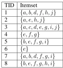
TID Itemset

1 fa;b;d;f;h;jg

2 fa;e;h;jg

3 fa;c;d;e;g;i;jg

4 fe;f;gg

5 fb;e;f;g;ig

6 feg

7 fa;b;d;f;g;ig

8 fb;e;f;g;h;ig

Table 4.1: Example transaction database

The nodes of the lexicographic tree can be generated in a top down recursive manner by

generating children of the root node and then generating the sub-trees rooted at these child

nodes.

We therefore need a representation for transaction databases that allows such a top down

recursive generation of the lexicographic tree. The use of projected databases provides such

a representation. The sub-tree rooted at a node in the lexicographic tree representing a

transaction database D can be generated from an -projected database of D. Projected

databases are examined in detail in this section.

We present the concept of projected databases with an example as follows. The

trans-action databaseDlisted in Table 1.2 will be used here.

Here C = fa;b;c;d;e;f;g;h;i;jg. The lexicographic order, R, chosen over C is

(a;b;c;d;e;f;g;h;i;j). Itemsets in the transactions inDordered byRare shown in Table

4.1.

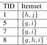
Given an itemsetordered byR, the-projected database ofD, w.r.t. the orderR, is

obtained from the set of transactions inDthat contain. For example, ifis the itemset

(28)

TID Itemset 1 fh;jg

5 fg;ig

7 fg;ig

8 fg;h;ig

Table 4.2:fb, fg-projected database

These are the only transactions inDwithfb;fgas subset.

The itemsets in the-projected database ofDw.r.t the orderRare the subsets of

trans-actions in D containing, such that every item in the subset occurs is infollow( ;R ).

The itemsets in thefb;fg-projected database ofDw.r.tR, are the subsets of transactions

1;5;7and8, consisting of items that occur afterf in the orderR. Thefb;fg-projected of

Dis shown in Table 4.2.

We formalize the notion of projected databases in the next section.

4.4.1 Formalization of Projected Databases

Choose a lexicographic orderR. Consider two itemsetsA;B 2I. OrderAandB

accord-ing toR. The(itemset)projectionofBonAw.r.t.R, denoted as I

(B;A;R ), is defined

as the setC B such thatC =B\follow(A;R ).

The (transaction)projection of a transactiont 2 T on an itemset 2 I w.r.t. R,

denoted by T

(t; ;R ), is defined as a transaction t 0

2 T such that t 0

:tid = t:tid and

t 0

:itemset= I

(t;itemset; ;R ).

The(database) projectionof a transaction databaseD on an itemset 2 I w.r.t the

orderR, denoted by DB

(D; ;R ), is defined as the transaction database which is the set

(29)

DB

(D; ;R )=f T

(t; ;R )jt2Dg.

DB

(D; ;R )is also denoted asD

(R ). WhenRis clear from context, DB

(D; ;R )

is abbreviated toD .

is called the prefix ofD

(R ).

For example, the transactions in databaseD in Table 4.1 are ordered according to the

orderR,(a;b;c;d;e;f;g;h;i;j).

Transactions1;5;7and8havefb;fgas prefix.

The projection of the itemset(fa;b;d;f;h;jgonfb;fgis:

I

(fa;b;d;f;h;jg;fb;fg;R )=fh;jg.

The transaction projection of transaction1onfb;fgw.r.tRis(1;fb;fg).

Thefb;fg-projected database ofD, DB

(D;fb;fg;R )orD fb;fg

(R ), is the set of

trans-action projections of transtrans-actions1;5;7and8, as shown in Table 4.2.

An -projected database, D

(R ) along with its prefix contains all the information

necessary to generate the nodes in the lexicographic tree that represent itemsets inI(D).

Along with,D

contains the all the information needed for mining itemsets with as

prefix fromD, whenDis being mined using the orderR. In the example above, thefb;fg

-projected database contains all the information needed for mining itemsets containingb;f

and items infollow(fb;fg;R ).

Thefb;fg-projected database can be obtained fromDsuccessively as follows:

1. Create thefbg-projected database ofD,D fbg.

2. Create theffg-projected database ofD fbg

(R )to getD fb;fg.

Formally, let A be an itemset fa 1

;a 2

;:::;a k

g, where jAj = k and A 0

be the itemset

fa 1

;a 2

;:::;a k 1

g.

Then DB

(D;A;R )can be obtained from DB

(D;A 0

;R )as DB

( DB

(D;A 0

;R );a k

(30)

If all itemsets in I(D)are enumerated using orderR overC, every itemset that starts

withcan be mined usingD

(R )and. This is done by prependingto itemsets mined

fromD

(R ).

4.5 Mining the

N

best itemsets using Projected Databases

In the preceding sections it has been shown that given an itemset 2 I(D), the nodes in

the subtree of the lexicographic tree rooted atcan be generated from D

. This property

is used to enumerate all such nodes of the lexicographic tree as follows.

Let S = fi 1

;i 2

;:::;i k

g C be the set of all items that occur inD

. The utility of

the itemset f [ig for each i 2 S, U(f[ig;D) is calculated and f [ig-projected

databases, D

f[ig are generated. Each

f[ig-projected database is recursively mined in

the same way, to generate and evaluate all the itemsets inD .

The algorithm util nbest pdb is presented below. It is a detailed version of the

util nbest outline algorithm, which uses the projected database representation. This

algorithm uses the recursive functionutil mine nbest pdb which enumerates and

calculates the utility of every itemset in a projected database.

Algorithmutil nbest pdb

Inputs

(31)

Method

1. Create a size-bounded priority-queue of sizeN. pq N

=create(N).

2. Callutil mine nbest pdb(D

(R );U;pq N

)

3. Returnpq N

:rankElements().

Algorithmutil mine nbest pdb

Inputs

1. The projected database to be mined,D

(R )

2. Utility function,U

3. A size-bounded priority queuepq N

Output The size-bounded priority queuepq N

Method

1. LetS be the set of all items that occur infp D

(R ). Let S = fi 1

;i 2

;:::;i k

gwhere

jSj=k.

2. For each item,i2Sdo

(a) CalculateU(f[ig;D).

(b) Set the priority of the itemsetf[igtoU((f[ig;D).

(c) pq N

:insert((f[ig).

(32)

(e) Generate projected databaseD f[ig

(R ).

3. Mine eachD f[ig

(R )by callingutil mine pdb(D

fal pha[ig

(R );U;pq N

).

4. Returnpq N.

4.6

Chapter 5 Utility Guided Pattern Mining using FP-Trees

In this chapter, we discuss implementation details of projected databases. We implement

projected databases using FP-Trees.

Given an-projected databaseD

(R ), anf[g-projected database,D f[g

(R )for

any follow( ;R )can be constructed fromD

(R ). In this chapter we will examine

how the FP-tree representingD f[g

(R )is obtained from the FP-Tree representingD

(R ).

We will also presentutil nbest fp, an algorithm that minesN best itemsets using

FP-Trees.

5.1 Implementation of Projected Databases

Agarwal et al in [1] use the bitmap representation of transaction databases and suggest a

hy-brid breadth-first, depth-first approach for the generation of projected transaction databases.

This way of representing transaction databases and the method for generating projected

databases suffers from the drawback of copying the entire transaction database and more

into the memory. This algorithm performs better than the apriori algorithm for generation

(34)

Han et al present the FP-Tree data structure for frequent pattern mining in [9]. A

frequent pattern tree, or FP-Tree for short, is an extended prefix tree structure used to

compactly represent transaction databases. A FP-Tree is constructed to represent the

trans-action database. It is mined by generating conditional pattern bases, constructing FP-Trees

for the conditional pattern bases and recursively mining them. The conditional-pattern base

is a sub-database which consists of sets of frequent items co-occurring with the suffix

pat-tern. An ordering over the catalog of items is chosen while constructing the FP-Tree. A

conditional-pattern base differs from a projected transaction database in that the items that

occur in the conditional-pattern base of a suffixall precede the items inin the ordering

used.

The principal benefits of the FP-Tree method of mining frequent patterns are the

fol-lowing:

Mining frequent patterns using FP-Trees takes only two passes over the

trans-action database, one for counting the support of single items and another for

constructing the FP-Tree, as against the Apriori algorithm and its variants,

where the number of passes over the transaction database is equal to the length

of the longest frequent pattern.

The FP-Tree representation does away with candidate generation, which causes

a combinatorial explosion in the Apriori algorithm and its variants.

Counting support is a significant overhead for Apriori and its variants as well

as the tree projection algorithm in [1]. Support information is maintained in

the FP-Tree and the support counting overhead is done away with.

Conditional pattern bases are conveniently generated from FP-Trees and

com-pactly stored in the memory. Generation and storage of projected databases

(35)

significantly better than Apriori.

To avail of these significant benefits, we use FP-Trees for the representation of projected

databases. We discuss the use of FP-Trees to represent projected databases in the following

section.

5.1.1 Representation of Projected Databases using FP-Trees

We use FP-Trees to represent projected databases. The representation of projected databases

using FP-Trees is formalized in this section.

Consider the -projected database of D, w.r.t. an orderR, D

(R ). The FP-Tree

rep-resenting D

(R ) is constructed from the transactions in D

(R ). The order R is used to

construct the FP-Tree. We denote this FP-Tree byfp D

(R ).

The FP-Tree representing D is denoted by fp D

(R ), where R is the order used while

constructing the FP-Tree.

The projected databaseD

(R )is represented by the two tuple( ;fp D

(R )).

Dis represented by the two tuple(;fp D

(R )).

Itemsets of the formf[gare mined fromD

(R )as follows. The itemsetis mined

fromfp D

(R )andis prepended to it to obtain the itemsetf[g.

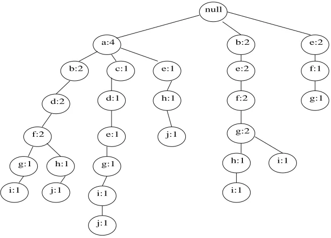
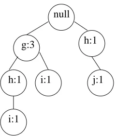
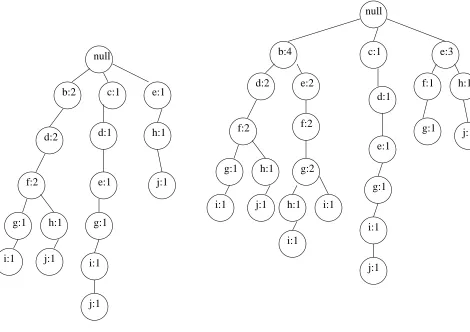
The FP-Tree for the transaction database D, from Table 4.1, is shown in Figure 5.1.

The FP-Tree for the fb;fg-projected database of D is shown in Figure 5.2. The itemset

fb;f;igis mined by mining the itemsetfigfrom this FP-Tree and prependingfb;fgto it.

5.2 Constructing the FP Tree for a projected database

Consider first the problem of obtaining the FP-Tree for an -projected database D

(R ),

fp D

(R ) from the FP-Tree representing D, fp D

(R ). The projected database D

(36)

a:4

f:2

b:2 c:1

d:1

e:1

g:1

i:1

j:1

e:1

h:1

j:1

b:2

e:2

f:2

g:2 null

e:2

f:1

g:1 d:2

i:1

h:1 i:1 g:1 h:1

i:1 j:1

Figure 5.1: FP-Tree for the transaction database in Table 1.2

h:1 i:1

i:1

h:1 g:3

null

j:1

(37)

obtained from those transactions inDthat haveas a prefix. These transactions are

rep-resented in fp D

(R ) by paths containing . Consider for example, the construction of

the fb;fg-projected database of the transaction database D in Table 1.2. This projected

database is obtained from transactions inDcontainingfb;fg. These transactions are

rep-resented in the FP-Tree in Figure 5.1 by paths containingfb;fg.

The-projection of a transactiontinDis obtained ast:itemset\follow( ;R ).

There-fore, given an FP-Tree,fp D

(R ), the set of all the sub-trees rooted at the last item in

con-tains the set of all itemsets in D

(R ). For the example above, the subtrees rooted at f in

paths containingfb;fgin the FP-Tree represent transactions inD fb;fg

(R ). These subtrees

when merged into a single FP-Tree representD fb;fg

(R ).

The FP-Tree D

(R ) can therefore be obtained by merging such subtrees into one tree

rooted at a null node.

Let = f 1

; 2

;:::; n

g, where j j = n. The FP-Tree, fp D

(R ) is obtained from

fp D

(R )by traversing all the paths infp D

(R )which containand combining the subtrees

rooted at

non these paths into a single FP-Tree.

Likewise, given a-projected database( ;fp D

(R )), for 2Isuch that =f 1 ; 2 ;:::; m g

wherejj= m, the FP-Tree fp D

[

(R )is obtained from fp D

(R )by traversing all paths

infp D

(R )that contain and combining the subtrees rooted at

m on these paths into a

single FP-Tree.

The problem of constructingfp D

(R )fromfp D

(R )therefore consists of two

subprob-lems, of finding all paths in fp

D that contain

and of creating an FP-Tree obtained by

merging subtrees rooted at

(38)

5.2.1 Merging Two FP-Trees

An FP-Tree stores itemsets that occur in the transaction database it represents and their

frequency counts. Two FP-Trees can be combined into one, by merging them. In the

merged FP-Tree, an itemset that occurs in both trees is represented by a single path, with

a frequency count that is the sum of the frequency counts in the two trees. An itemset that

occurs in only one tree is represented in the merged tree by a path and a frequency count of

the itemset in the single tree.

When two FP-Trees, fp D

(R ) and fp D

0

(R ), representing the transaction databases D

andD 0

are merged, the FP-Tree obtained represents the transaction database(D[D 0

). It

is denoted byfp (D[D

0 )

(R ).

The algorithmmerge is presented below. It merges two FP-Trees with the same item

at the root node. Given two FP-Trees,fp D

(R ) andfp D

0

(R ), letr be the root offp D

(R )

andr 0

be the root offp 0 D

(R ). The algorithmmergemerges the tree rooted atrinto the tree

rooted atr 0

such that the tree rooted atr 0

now represents the transaction databaseD[D 0

and

therefore is the treefp (D[D

0 )

(R ). The algorithm recursively merges subtrees as follows. It

starts with the trees rooted atrandr 0

. For each childaofr, it checks ifr 0

has a child node

that also representsa:item. If such a child, sayb exists, the frequency information stored

ina,a:frequencyis added tob:frequency. Ifr 0

does not have such a child, a new nodeb

identical toais created and made the child ofr 0

. The nodebnow represents an occurrence

ofa:iteminD[D 0

. The functionmergeis called recursively on the subtrees rooted ata

andb, to transfer information present in thea-subtree into the subtree rooted atb.

Algorithmmerge

Inputs

Roots noderandr 0

of FP-Treesfp D

(R )andfp D

0

(R )that are to be merged.

(39)

The FP-Treefp (D[D

0 )

(R ).

Method

1. Ifr:item6=r 0

:itemexit.

2. LetA=fa 1

;a 2

;:::;a k

gbe thekchildren ofrin the orderR.

LetB =fb 1

;b 2

;:::;b k

gbe thekchildren ofr 0

in the orderR.

3. For each nodea2Ado

(a) Search for a nodebinB such thata:item=b:item.

(b) If such a node does not exist

i. Create a new nodeb =(a:item;a:frequency).

ii. Insertbas a child ofr

2 according to order R.

else if such a node exists, call itb. Dob:frequency=b:frequency+a:frequency.

(c) Callmerge(a;b).

4. Return the FP-Tree rooted atr 0

.

Analysis of Algorithmmerge

Let the number of nodes infp D be

Z. Thenmergetakes timeO(Z).

5.2.2 Constructing a projected database

As discussed in Section 5.2, given ; 2 I(D), D [

(R ) can be obtained fromD

(R ),

by finding all paths infp D

(R ) that contain and merging the subtrees rooted at the last

(40)

The algorithmprojectis presented below. Given an FP-Treefp D

(R )and an itemset

, Algorithmprojectreturnsfp D

[ (R ).

The algorithm starts by creating a null node as the treefp D

[

(R ). Let =f 1 ; 2 ;:::; m g,

wherejj =m. Each path containing infp D

(R )is found and the subtree rooted at m

is merged onto the FP-Tree,fp D

[

(R ), constructed thus far.

Algorithm project Inputs

1. The FP-Treefp D

(R ).

2. An itemset 2I such that =f 1

; 2

;:::; m

g, wherejj=m

Output

The FP-Treefp D

[ (R ).

Method

1. Create a new null node,root

new, as root of the FP-Tree FP

D [

(R ).

2. Letrootbe the root ofFP D

(R ).

3. Find each occurrence of inFP D

(R ) and merge the subtree under the node m

intofp D

[

.

This is done by callingfind and merge(root;root new

; 1

;;R ).

The algorithmfind and mergeis described below.

Algorithmfind and merge

Inputs

(41)

2. The root,root

new, of the new FP-Tree into which the subtrees are to be merged.

3. The item,key, currently being matched.

4. The entire itemset,pattern, currently being matched

5. The order,R, used for constructing the FP-Trees rooted atrootandroot new.

Output

The FP-Tree rooted atroot new.

Method

1. Ifkey=nullreturnroot.

2. Let child nodes ofroot,Child =fchild 1

;child 2

;:::;child k

g

3. Forifrom1tokdo

(a) ifroot:item=key

i. key

new= the item in

patternnext afterkey.

ii. ifkey=null,merge(root;root new

).

elsefind and merge(child i

;root new

;key new

;pattern;R ).

iii. Returnroot new.

(b) find(child i

;root new

;key;pattern;R ). returnroot new.

Analysis of the algorithm LetZ be the number of nodes inf D

(R). Then the algorithm

find and mergetakes timeO(Z). The find and mergealgorithm consists of

two components, finding paths in the FP-Tree that contain and of merging the subtree at

that path into the FP-Tree being constructed for thef[g-projected database. Both these

(42)

h:1 null

g:1

i:1 j:1

Figure 5.3: Merge of null FP-Tree and tree under(a:2;b :2;d:2;f :2)in Figure 5.1

Example Consider the FP-Tree in Fig 5.1. The FP-Tree for thefb;fg-projected database

is constructed fromfp D

(R ) according the the algorithmproject as shown in the Figures

5.3 and 5.4. A null node,root

new, is created to represent fp

D fb;fg

(R ). The subtree under

the nodefin the path(a:2;b:2;d:2;f :2)is merged with this tree as follows: The node

f has2children,g andh. Sinceroot

new does not have a child

g, a newg node is created

underroot. Now the subtrees rooted at the twog nodes are merged. Theg node underf

has a child h, whereas the g node under root

new does not. A new

h node is created and

inserted under this g node. The merging thus continues till the FP-Tree shown in Figure

5.3 is obtained. The subtree under path(b :2;e :2;f :2)is then merged withfp D

fb;fg (R )

to get the FP-Tree shown in Figure 5.4.

5.3 Mining the

N

best itemsets using FP-Trees

In Section 5.2, we discussed the construction of the FP-Tree fp D

(R ) representing the

projected database D

(R ). All itemsets of the form ( [) where follow( ;R )

can be enumerated using D

(R ) and , therefore using fp D

(R ) and. In this section

(43)

h:1 i:1

i:1

h:1 g:3

null

j:1

Figure 5.4: Merge of tree in Figure 5.3 and tree under(b :2;e:2;f :2)inFigure5:1

to enumerate all the itemsets contained in D

(R ). We discuss a property of FP-Trees in

Section 5.3.1 that allows efficient splitting up of an FP-Tree into FP-Trees that represent

projected databases of children of its root node. This property is then used in Section 5.3.3

to present the version ofutil nbest pdbthat uses FP-Trees.

5.3.1 Child Projected Databases

Let q be a node in the FP-Tree fp D

(R ). The item and frequency information stored in

subtree rooted at q is needed during the mining of the subtrees rooted at its siblings that

are to the right of q, that is its siblings that represent items in follow(q:item;R ). This

information is not needed in mining the subtrees rooted at its siblings to the left.

If qis the left-most child of a nodep, the frequency information in the subtree rooted

atq can be transferred out into the subtrees to its right under nodep. The tree rooted atq

can then be cut out from underp. IfI is the itemset on the path from the root to node p,

the cut out sub-tree rooted atq represents thefI[qg-projected databaseD fI[qg

(R ). The

algorithmmergediscussed in Section 5.2.1 is used to transfer information from the subtree

(44)

Example

Consider the FP-Tree in Figure 5.1. The leftmost child of the null root node is a.

The item and frequency information stored in the subtree rooted at a is necessary while

constructingb;c;:::;j-projected databases. This information can be transferred from the

a-rooted tree into subtrees under the null root as follows. The sub-tree rooted at nodeais

cut out from under the null root. This subtree represents thea-projected database. The root

anode is replaced by a null root node. This new tree is merged with the original FP-Tree.

That is, the b subtree under the new root is merged with the b subtree under the old null

root. A newcsubtree is created under the old null root and the esubtree in the new tree

is merged with theesubtree under the old null root. Thea-projected database can now be

mined independently of the rest of the FP-Treefp D

(R ).

Now the leftmost child under the null root of fp D

(R ) is theb-node. Theb-projected

database can be cut out of the FP-Treefp D

(R ) as explained earlier. This process can be

repeated with other children of the null root node offp D

(R ), untilfp D

(R )is split up into a

number of child projected databases. Each projected database can be mined independently

of the rest. Thus the original FP-Tree is replaced by FP-Trees representing the projected

databases of the children of its root.

This splitting up of the FP-Tree is formalized as follows.

If S C is the set of all items that appear in D

, then the children of the null-root

node offp D

(R )are the items inSordered byR. LetS =fi 1

;i 2

;:::;i k

gwherejSj=k.

Then FP D

(R ) can be split up into k FP-Trees representing the k projected databases

D f[i 1 g ;D f[i 2 g

;:::;D f[i

k g.

The algorithm,split fpis presented below. The algorithm takes the FP-Tree for an

-projected database,fp D

(R )as input. It splitsfp D

(R )into FP-Treesfp D

f[i 1

g

(R );:::;fp D

f[i k

g (R ),

wherei 1

;:::;i

k are the items that appear in D

(45)

the leftmost subtree, rooted at the node lchild, out offp D

(R ). The lchild root node in

this cut out subtree is replaced by a new null node. This FP-Tree represents thef[i 1

g

-projected database. The frequency information stored in this subtree is transferred to the

remainder of fp D

(R ). The algorithm merge is used for this purpose. The process is

repeated with the other children.

Algorithmsplit fp

Inputs

A FP-Tree,fp D

(R ).

Output

FP Trees representing the projected databasesD f[i

1 g

;D f[i

2 g

;:::;D f[i

k g.

Method

1. Setrootto be the null-root ofFP D.

2. While theroothas children do

(a) Letlchildbe leftmost child node ofroot.

(b) Letli=lchild:item.

(c) Cut out the subtree rooted atlchildfrom underroot. Replace the root node of

this subtree,lchildwith a new null root node,root new.

This subtree is the FP-Tree,fp D

f[lig (R ).

(d) Callmerge(root new

;root).

(e) While merging, thread both trees appropriately.

(f) Outputfp D

f[lig (R )).

(46)

b:2 e:1 null

f:2 d:2

g:1 h:1

i:1 j:1

c:1

d:1

e:1

g:1

i:1

j:1

h:1

j:1

h:1

j:1 g:1

e:3

f:1 d:1

e:1

g:1

i:1

j:1 c:1 b:4

f:2 d:2

g:1 h:1

i:1 j:1

e:2

f:2

g:2

h:1 i:1

i:1

null

Figure 5.5: Thea-projected database cut out of the FP-Tree in Fig 5.1

The cutting out of thea-projected database from the FP-Tree in Fig 5.1 is shown in Fig

5.5.

Analysis of the algorithmsplit fp

Let the number of nodes infp D

(R )beZ. Thesplit fptakesO(Z)time. This is because

split fpcuts subtrees out of the input FP-Tree one by one and uses themergealgorithm

to transfer information out of them. Themerge algorithm takes time of the order of the

number of nodes in the FP-Tree it receives as input. Cutting out a subtree from an FP-Tree

(47)

The maximum space that the split FP-Trees generated by this algorithm occupy is

O(2 N

), where N = jCj. Though the total space required by the smaller FP-Trees can

be greater than the original FP-Tree, we expect the space required by the split up trees to

beO(Z). The original FP-Tree is replaced by a set of smaller split-up FP-Trees.

5.3.2 Comparison of

split fp

with

fp growth

In this section we provide a detailed analysis of the time complexity of splitting an FP-Tree

into smaller trees representing child projected databases of the null root node. We compare

the time taken by split fp to the time taken by thefp growth algorithm presented

in [9] would take to for the task of generating the child projected databases of FP-Tree’s

root node. Such a comparison is pertinent, because thefp growthalgorithm mines the

FP-Tree for frequent patterns by successively generating smaller FP-Trees that represent

conditional pattern bases. Conditional pattern bases are analogous to projected databases.

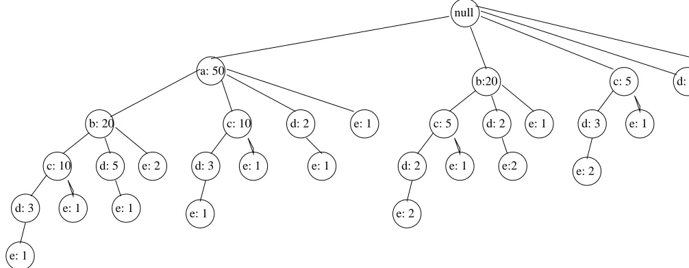
For the analysis we assume that every itemset in I occurs in the transaction database

D. The FP-Tree constructed for such a transaction database is maximal in the sense that

contains every possible path and node. Figure 5.6 illustrates one such maximal FP-Tree for

the catalogC =fa;b;c;d;eg.

The number of nodes accessed bysplit fpwhile splitting such a maximal FP-Tree is

O(2 N

), whereN =jCj, as there are2 N

1nodes in the maximal FP-Tree. Thus the worst

case performance ofsplit fpisO(2 N

).

Given an FP-Treefp D

(R )and an itemi2C,fp growthgenerates the FP-Tree for the

fig-projected database as follows. It travels up the subpath that starts from an occurrence of

iin the tree to the root node to obtain thefig-projected transaction, also called conditional

pattern, represented by the subpath. It obtains the set of all such conditional patterns by

(48)

an the FP-Tree representing thefig-projected database ofD.

The number of nodes accessed by fp growth while generating the fig-projected

databases for all i 2 C, for a maximal FP-Tree such as the one shown in Figure 5.6 is

calculated as follows. The total number of nodes accessed is summation of the number of

nodes at each level of the tree times the number of nodes on a path from that level to the

root.

Number of nodes accessed

= P N m=1 C N m (m 1) =2 N N 2 +1

Therefore the worst-case time taken byfp growthisO(N2 N

).

Thesplit fpalgorithm isO(N)faster than thefp growthalgorithm.

In general, if the nodes in an FP-Tree have an average depthdand the average branching

factor in the tree isb,split fptakes timeO(b h

). Thefp growthalgorithm takes time

O(db d

).

5.3.3 Algorithm

util nbest fp

using FP-Trees

All itemsets of the form([)where 2I(D

(R ))can be enumerated fromfp D

(R ).

We examine projected databases successively using the algorithmsplit fpfor this

pur-pose as follows. If fi 1

;i 2

;:::;i k

g is the set of all items that occur in D

(R ), we split

fp D

(R )into FP-Trees repfp D

f[i 1

g

(R );:::;fp D

f[i k

g

(R ). The itemsetsf [i 1

g;:::;f [

i k

gare generated while splittingfp D

(R ). The utility of these items is calculated. We

re-cursively split up and mine each generated FP-Tree using split fp until the projected

databases of all itemsets in I(D

(R ))have been generated and evaluated. The algorithm

(49)

e: 1 e: 1 b: 20 e: 2 a: 50 c: 10

d: 3 e: 1

e: 1 d: 2 d: 5 e: 1 c: 10 d: 3 b:20 e: 1 e: 2 e: 1 d: 3

c: 5 d: 5

e: 1 e: 1 e: 1 null e:2 d: 2 c: 5 d: 2 e: 2

Figure 5.6: A maximal FP-Tree

itemset inI(D

(R )). It uses FP-Trees to implement projected databases. It is a

modifica-tion of the algorithmutil mine nbest pdb.

Algorithmutil mine nbest fp

Inputs

1. The FP-Tree to be mined,fp D

(R ).

2. The utility function,U.

3. A size-bounded priority queuepq N

Output The size-bounded priority queuepq N

Method

1. LetS be the set of all items that occur infp D

(R ). Let S = fi 1

;i 2

;:::;i k

gwhere

jSj=k.

(50)

(a) CalculateU(f[ig;D).

(b) Set the priority of the itemsetf[igtoU(f[ig;D).

(c) pq N

:insert(f[ig).

3. Splitfp D

(R )intokFP-Trees representing the projected databasesD f[i

1 g

;:::;D f[i

k g.

4. Mine eachfp D

f[ig

(R )by callingutil mine nbest fp(fp D

f[ig

(R );U;pq N

).

5. Returnpq N.

We now present the algorithmutil nbest fpthat returnsN itemsets with best utility

values using FP-Trees.

Algorithmutil nbest fp

Inputs

Output

Method

1. Create a size-bounded priority-queue of sizeN.

pq N

=create(N).

2. Choose an orderRover items inC, that will be used to constructfp D

(R ).

3. TraverseDonce and constructfp D

(51)

4. Callutil mine nbest fp(fp D

(R );U;pq N

).

5. Returnpq N

:rankElements().

Analysis of the algorithm Every itemset is enumerated by the algorithm. Therefore,

theI-projected database is constructed for eachI 2I(D). To calculate the time taken by

util nbest fp, we consider the maximal FP-Tree presented in Figure 5.6. Since the

I-projected database is generated for everyI 2I(D), the sum of all nodes accessed by the

algorithm is calculated as follows. Order all items inC byR.

P N m=1

Number of occurrences of themth item ofC in the FP-TreeNumber of nodes

in the subtree rooted at themth item.

Therefore, the number of nodes accessed

= P N m=1 2 (m 1) 2 N m = P N m=1 2 (N 1)

=N 2 (N 1)

The algorithmutil nbest fpmakes only one path over the transaction database.

The time taken byutil nbest fpisO(N 2 N

)for the maximal FP-Tree. This is

the worst-case performance time of the algorithm. The space used isO(2 N

).

For an FP-Tree with an average branching factorband where the nodes have an average

depth ofd, the time taken isO(db d

). The space used by the algorithm isO(b d

).

Example The algorithm util mine fp is explained with the help of an

exam-ple. For the transaction database D in Table 1.2, let the utility function be defined as

U(I;D)=revenue(I;D)for anyI 2I(D). Consider the mining of thefb;fg-projected

database shown in Figure 5.2. The items that occur in D

fb;fg are

S = fg;h;i;jg. The

utility values,U(fb;f;gg;D),U(fb;f;hg;D),U(fb;f;ig;D)andU(fb;f;jg;D)are

(52)

prices ofb;f andg are3;5and2respectively, thenprice(fb;f;gg;D) =10. The support

of fb;f;gg is available from the FP-Tree, support(fb;f;gg;D) = support(fgg;D fb;fg

).

Therefore,U(fb;f;gg;D)=103=30.

The FP-Tree in Figure 5.2 is split up into thefb;f;gg, fb;f;hg,fb;f;igandfb;f;jg

projected databases and each of them is mined recursively till all itemsets in D

fb;fg have

been enumerated and evaluated.

5.4 Related Work

In the preceding sections, we have discussed the problem of enumerating all itemsets in

I(D)and calculating their utility. Enumerating all itemsets in I(D) is equivalent to

fre-quent pattern mining with a support threshold of one. In this section various methods in

the literature for frequent pattern mining are compared to theutil nbest fpalgorithm,

which splits FP-Trees into child projected databases successively and mines the FP-Tree in

a top-down fashion.

The Apriori algorithm presented in [3] mines frequent patterns using a generate and

test paradigm. Candidate patterns of length k +1 are generated from frequent patterns

of length k in the k +1st iteration of the algorithm. The support of candidate itemsets

generated is counted by one pass over the transaction database. The itemsets identified as

frequent from amongst the candidates are used in the next iteration as discussed before. A

complete traversal of the transaction database is made at every iteration of the algorithm.

The total number of iterations over the transaction database is equal to the length of the

longest pattern. A very large number of candidate patterns are generated. The storing

and support counting of a large number of candidate itemsets is expensive. The Apriori

(53)

The tree projection algorithm presented in [1] does away with candidate generation by

using a lexicographic tree to enumerate frequent itemsets. The lexicographic tree is

gen-erated using projected databases in a breadth first, depth first or a hybrid of breadth and

depth first methods. A bitmap representation is used for projected databases. The

breadth-first approach suffers from the drawback of having to make one traversal of the transaction

database per iteration of the algorithm and from expensive support counting. The

depth-first approach makes support counting easier and localized to the projected database. It

suffers from having to maintain projected databases at all nodes along the path being

ex-amined. The hybrid approach of using breadth first generation for the initial levels of the

tree and the depth first approach at lower levels mitigates these drawbacks to a certain

ex-tent. The hybrid tree projection algorithm has performance similar to Apriori at higher

support thresholds, but outperforms Apriori at lower support thresholds. Significant

contri-butions made by this paper are the concepts of lexicographic tree and projected databases,

which do away with candidate generation and counting.

The frequent pattern tree is presented as a way to represent transaction databases in

[9]. Candidate generation is done away with. The number of passes over the transaction

database is limited to two. During the first pass, the support of singleton itemsets is

cal-culated. An ordering that arranges items in the descending order of support is chosen to

construct the FP-Tree. Items with greater support lie at the higher levels of the tree as

com-pared to items with lower support. The FP-Tree is mined recursively in a bottom up manner

by the FP Growth algorithm using the concept of conditional pattern bases. The FP-Tree

method of mining frequent itemsets is faster than Apriori and Tree Projection, even at low

support threshold levels.

Ourutil mine fpalgorithm mines FP-Trees in the top down manner usingsplit fp

Utility Guided Pattern Mining

Abstract

UTILITY GUIDED PATTERN MINING

Biography

Table of Contents

List of Tables

List of Figures

Chapter 1

Introduction and Motivation

1.1

Introduction

1.2

Motivation

1.3

Examples

Chapter 2

Terminology and Definitions

Chapter 3

Formulation Of Pattern Mining Problems Using

Utility Functions

Chapter 4

Pattern Mining using Utility Functions

4.1

Ranking Itemsets by Utility

4.1.1

Analysis of the Algorithm

4.2

Mining

itemsets with the best utility values

4.2.1

Size-bounded Priority Queues

4.2.2

Algorithm to mine

itemsets with best utility values

4.3

Lexicographic Tree of Itemsets

4.4

Projected Databases

4.4.1

Formalization of Projected Databases

4.5

Mining the

best itemsets using Projected Databases

4.6

Other Utility Guided Pattern Mining Problems

Chapter 5

Utility Guided Pattern Mining using FP-Trees

5.1

Implementation of Projected Databases

5.1.1

Representation of Projected Databases using FP-Trees

5.2

Constructing the FP Tree for a projected database

5.2.1

Merging Two FP-Trees

5.2.2

Constructing a projected database

5.3

Mining the

best itemsets using FP-Trees

5.3.1

Child Projected Databases

5.3.2

Comparison of

with

5.3.3

Algorithm

using FP-Trees

5.4

Related Work