E
NERGY
E
FFICIENT
TCP
Master’s thesis: L. Donckers
CAES/002/01
May, 2001
University of Twente
Department of Computer Science
Division: Computer Architecture and Embedded Systems
I
S
AMENVATTING
Een nieuw type handcomputer is in ontwikkeling in het Moby Dick project. Door de gewenste functionaliteit en prestaties, zal het energie verbruik de limiterende factor zijn voor deze handcomputer. Draadloze communicatie zal ook een belangrijke factor zijn in het project, wat een energie-efficiënt transport protocol, compatible met TCP/IP, wenselijk maakt. Dit verslag beschrijft het ontwerp van zo’n energie-efficiënt transport protocol voor mobiele draadloze communicatie.
Er is echter nog niet veel onderzoek gedaan naar de energie efficiëntie van transport protocollen. Daarom zijn er eerst maten ontwikkeld om de energie efficiëntie van transport protocollen te kunnen meten. Deze maten zijn gebruikt om de prestaties van TCP/IP op draadloze verbindingen nauwkeurig te bestuderen. Vier probleemgebieden zijn gedefinieerd, die TCP/IP ervan weerhielden een hoog niveau van energie efficiëntie te behalen. Voor deze probleemgebieden zijn mogelijke oplossingen aangedragen waarna de haalbaarheid er van is onderzocht.
III
A
BSTRACT
A new generation handheld computer is under development in the Moby Dick project. Because of the desired functionality and performance, the energy consumption will be the limiting factor for this handheld. Wireless communication will also be an important factor in the project, which makes an energy-efficient transport protocol, compatible with TCP/IP, desirable. This thesis describes the design of such an energy-efficient transport protocol for mobile wireless communication.
However, not much research has yet been done on the energy efficiency of transport protocols. First metrics were developed to measure the energy efficiency of transport protocols. These metrics were used to study the performance of TCP/IP on wireless links carefully. Four problem areas were defined that prevented TCP/IP from reaching high levels of energy efficiency. For these problem areas, solutions were proposed and their feasibility was examined.
V
T
ABLE OF CONTENTS
PREFACE VII
1 INTRODUCTION 1
1.1 PROBLEM AREA 1
2 MEASURING ENERGY EFFICIENCY 3
2.1 ENERGY EFFICIENCY AND ENERGY OVERHEAD 3
2.2 DATA OVERHEAD AND TIME OVERHEAD 4
2.3 POWER MODEL OF RADIOS 4
2.4 CALCULATING DATA OVERHEAD AND TIME OVERHEAD 6
2.5 CALCULATING ENERGY OVERHEAD 7
2.6 CALCULATING ENERGY EFFICIENCY 7
2.7 SUMMARY 9
3 ASPECTS OF TCP 11
3.1 TRANSPORT CONTROL PROTOCOL 11
3.1.1 RELIABILITY 11
3.1.2 SLIDING WINDOWS 11
3.1.3 ACKNOWLEDGEMENTS AND RETRANSMISSION 12
3.1.4 TIMEOUT AND RETRANSMISSION 12
3.1.5 WINDOW SIZE AND FLOW CONTROL 13
3.1.6 RESPONSE TO CONGESTION 13
3.2 PROBLEMS OF TCP 13
3.2.1 LARGE HEADERS 14
3.2.2 SIMPLE ACKNOWLEDGEMENT SCHEME 14
3.2.3 LOSS IS CONSIDERED CONGESTION 15
3.2.4 COMPLETE RELIABILITY 15
3.3 POSSIBLE SOLUTIONS 15
3.3.1 HEADER COMPRESSION 16
3.3.2 SELECTIVE ACKNOWLEDGEMENTS 17
3.3.3 DELAYED ACKNOWLEDGEMENTS 18
3.3.4 EXPLICIT CONGESTION NOTIFICATION 19
3.3.5 FORWARD ERROR CORRECTION 19
3.3.6 I-TCP 20
3.3.7 PROTOCOLS INSPIRED BY I-TCP 20
3.3.8 DELAYED DUPLICATE ACKNOWLEDGEMENTS 21
3.3.9 MOBILE-TCP 21
3.3.10 PRTP 21
3.3.11 OPTIMIZED WINDOW MANAGEMENT 22
VI
4 E2TCP 23
4.1 ARCHIT ECTURE OVERVIEW 23
4.1.1 HEADERS 23
4.1.2 ACKNOWLEDGEMENTS 23
4.1.3 WINDOW MANAGEMENT 24
4.1.4 RELIABILITY REQUIREMENTS 25
4.2 HEADER FORMAT 25
4.2.1 IP HEADER 25
4.2.2 TCP HEADER 27
4.2.3 E2TCP HEADER 29
4.2.4 E2TCP HEADER SIZES 33
4.3 SELECTIVE ACKNOWLEDGEMENTS 33
4.4 WINDOW MANAGEMENT 35
4.4.1 CONGESTION AND FLOW CONTROL 35
4.4.2 TRANSMISSION 36
4.4.3 RETRANSMISSION 36
4.4.4 ACKNOWLEDGEMENTS AND WINDOW SIZE 36
4.4.5 ROUND TRIP TIME ESTIM ATION 37
4.4.6 BURST ERROR DETECTION 37
4.5 PARTIAL RELIABILITY 39
5 TEST RESULTS 41
5.1 SIMULATION MODEL 41
5.2 TEST SETUP 41
5.3 ERROR MODEL AND SETUP 43
5.4 E2TCP PARAMETERS 44
5.4.1 MINIMUM WINDOW SIZE 44
5.4.2 MAXIMUM WINDOW SIZE 46
5.4.3 WINDOW SIZE AFTER A TIMEOUT 46
5.4.4 ERROR LIMIT 47
5.4.5 CONCLUSIONS 48
5.5 E2TCP DISSECTED 49
5.5.1 WINDOW MANAGEMENT 49
5.5.2 SELECTIVE ACKNOWLEDGEMENTS 49
5.5.3 E2TCP HEADERS 50
5.5.4 PARTIAL RELIABILITY 51
5.5.5 CONCLUSIONS 52
5.6 EVALUATION OF E2TCP 53
5.6.1 DEFAULT SETUP 53
5.6.2 BANDWIDTH 57
5.6.3 DELAY 58
5.6.4 TRAFFIC 59
5.6.5 PARTIAL RELIABILITY 61
5.6.6 PERFORMANCE 62
5.6.7 CONCLUSIONS 64
6 CONCLUSIONS AND RECOMMENDATIONS 67
VII
P
REFACE
I would like to take the opportunity to thank my supervisors: Gerard Smit, Paul Havinga and Lodewijk Smit for guiding me while I was working on this assignment. I would also like to thank my mother, brother and sister for being there for me. For the same reason I thank Ella, Jac and Jessie.
Last but certainly not least, I would like to thank my girlfriend: Lonneke. Without her support this would have been impossible.
Enschede, May 2001
1
1
I
NTRODUCTION
This thesis is part of the Moby Dick project at the Computer Science department of the University of Twente. The Moby Dick project is a joint European project to develop and define the architecture of a new generation of mobile handheld computers. Due to the increasing demand for performance and functionality, the energy consumption will be the limiting factor for the capabilities of such a new generation handheld. Therefore reducing energy consumption plays a crucial role in the architecture. An important aspect of the Moby Dick project is wireless communication. Because of the importance of energy efficiency to the Moby Dick project, the wireless communication should also be optimized to minimize energy consumption.
Unfortunately, not a lot of research has been done on energy-efficient transport protocols. Even though it would be quite rewarding to do so, because in mobile systems, the radio (which is used for wireless communication) is one of the parts that consume the most energy [STE97]. Computer chips (like CPUs and memories) are becoming increasingly energy efficient because of advances in IC design. Radios however simply require a certain amount of energy to transmit and receive information. Furthermore, multimedia applications are using network services more extensively and continuously than before. The impact of minimizing the energy spent on wireless communication, will therefore only increase [HAV00b].
For these reasons, it would be beneficial to the Moby Dick project if an energy-efficient transport protocol would be designed. As a basis for such a protocol, TCP/IP (Transport Control Protocol/Internet Protocol) is a likely candidate. This would enable the handheld to communicate, via the Internet, with vast numbers of systems.
This led to the following problem statement:
The energy efficiency of transport protocols on wireless links should be researched. Based on that research, E2TCP –an energy efficient version of TCP/IP– should be designed and implemented, to test its energy efficiency and performance.
The remainder of this chapter further delineates the problem area of E2TCP. Chapter 2 explains what energy efficiency is and how it can be calculated. Chapter 3 then describes TCP/IP, explains what keeps it from reaching high levels of energy efficiency and what can be done to remedy this. The solutions presented in Chapter 3 were used to design E2TCP, which is described in Chapter 4. In Chapter 5 an implementation of E2TCP will be introduced before a thorough energy efficiency and performance evaluation will be given. Finally Chapter 6 gives the conclusions of this thesis.
1.1
Problem area
E2TCP will be used on a wireless link between a mobile host and a base station. The mobile host should be able to connect to the Internet via the base station in such a way that it is transparent to the mobile host and the Internet host it is connected with. This means neither the mobile host nor the Internet host should be able to tell whether E2TCP is used between the mobile host and the base station or regular TCP/IP. (Because the behavior of TCP is highly dependant on IP, E2TCP will have the functionality of both TCP and IP. This maximizes the potential gain in energy efficiency.)
2
protocol will be used as a drop-in replacement for TCP/IP on the mobile host and should be usable on all wireless links, just like TCP/IP is usable on all wired networks. The protocol should therefore make no assumptions about the link- and MAC layers.
Now it is clear what should not be changed, it is time to explain what is allowed to be changed. There are three parts of the systems that can be changed. They are additive, which means that the second proposed change also includes the first and that the third proposed change also includes the second and first.
The first proposed change is to replace TCP/IP at the base station with E2TCP. This change requires no user intervention but it is expected that by only applying this change, the increase in energy efficiency is rather small.
The second proposed change is to also replace the transport protocol on the mobile host. This requires some user intervention because the user must install the protocol on its mobile host. Because of the user-friendliness of modern operating systems this should not be a big problem. When this proposal is executed a truly new transport protocol can be designed because it does not have to communicate directly with TCP/IP. A proxy application at the base station can then handle the translation of the energy efficient protocol on the wireless link to TCP/IP on the wired part of the path. The design of the proxy is not part of the problem statement: E2TCP will be the sole point of focus. It is expected that this proposal will yield an increase in energy efficiency compared to only the first change. Such a setup is shown in Figure 1.1.
E2TCP
link layer
MAC layer link layer
MAC layer
application application
mobile host internet host
TCP
IP E2TCP
link layer
MAC layer proxy base station
link layer
MAC layer TCP
IP
wireless link fixed link
Figure 1.1: The intended setup of E2TCP.
The third proposal is to change (some of) the applications on the mobile host as well. These applications will then be able to optimize the energy efficient connections for their intended use with Quality of Service-like (QoS-like) parameters. It is expected that this will increase the energy efficiency even further in certain cases, which would not have been possible with only the first two proposed changes.
The conclusion of this chapter is that the protocol should meet the following requirements:
• It should be a transport protocol and should be compatible with TCP/IP (through translation at the base station).
• It should be energy efficient.
• It should make no assumptions about the lower layers and leave them unchanged.
3
2
M
EASURING ENERGY EFFICIENCY
When researching the energy efficiency of protocols, it is of course important to know what exactly energy efficiency (of a protocol) is and how to calculate it. In this chapter both topics will be discussed.
2.1
Energy efficiency and energy overhead
Energy efficiency is a measure to indicate how much energy a protocol uses to transmit data (in a certain case) compared to an ideal protocol. It will not be measured in absolute values because different cases (with different amounts of payload) should be comparable. An energy efficiency near 0% means little of the spent energy was used efficiently, while an energy efficiency of 100% means that no energy was wasted, which can only be achieved by an ideal protocol.
It is important to know that for a given data transmission medium there is a minimum amount of energy that is required to send data from source to destination. No protocol can use less energy and still successfully complete the transmission. Let's call this minimum M. This is probably different from the actual spent energy, called S. The difference between those two values is called W; the amount of wasted energy. These values are shown in Figure 2.1.
S
M W
S = energy Spent by the protocol W = energy Wasted by the protocol
M = Minimum amount of spent energy possible +
=
Figure 2.1: The relation between the spent, wasted and minimum amount of energy.
Energy efficiency then is:
EE = M / S
Equation 2.1: Energy efficiency.
or in words: the part of the spent energy that was used useful. If the protocol is ideal and it only uses the minimum amount of energy (S = M) the energy efficiency is 100%. Since M is fixed and S can only increase, the energy efficiency can only become lower.
Even though this is exactly what is needed to know about the protocols in this assignment, energy efficiency is not a good way to compare various protocols. This is because the differences in energy efficiency will be quite small even though the amount of wasted energy can differ quite much. Consider the following example.
4
energy as protocol A (W is 50 and 25 respectively). But the energy efficiency of protocol A is 100 / 125 = 80% and that of B is 100 / 150 = 67%. When one only looks at the energy efficiency it is easy to see that protocol A is better than protocol B. When one tries to see how much protocol A is better, the energy efficiency numbers are not that convenient.
There is another measure that is closely related to energy efficiency: energy overhead. Energy overhead is the amount of wasted energy compared to the minimum amount of energy, or:
EO = W / M
Equation 2.2: Energy overhead.
This can be seen as the amount of energy that is spent more than the minimum the protocol requires. Because of its close relation with energy efficiency, energy overhead can be calculated when only energy efficiency is known, and vice versa. Unlike energy efficiency however, energy overhead is more suited to show the differences between two protocols. This is shown in the next example.
Example 2.2: Consider the previous example but now the energy overhead will be calculated instead of energy efficiency. The energy overhead of protocol A is 25 / 100 = 25% and the energy overhead of protocol B is 50 / 100 = 50%. This shows precisely that protocol B wastes twice as much energy as protocol A.
Energy overhead will be used to compare protocols from now on, while energy efficiency numbers will sometimes be stated to be complete.
2.2
Data overhead and time overhead
Now a definition of energy overhead has been given, it is time to show how it is calculated. Before this can be done it is important to understand what precisely influences the energy efficiency and overhead of a protocol. Basically there are two characteristics that influence them. The first characteristic is the data overhead of a protocol. When a protocol uses more bytes to transmit the same amount of data, more bytes are wasted. Therefore the protocol becomes less energy efficient. The second characteristic that influences the energy efficiency of a protocol is time overhead. In certain cases, the longer the protocol needs to transmit the same amount of data, the longer the radio has to be active. When the radio is active, it requires (extra) energy to operate. Thus, the more time a protocol requires to send the same amount of data, its energy efficiency decreases. These two characteristics are sometimes related.
The question remains how much these characteristics each influence energy efficiency. The answer really depends on the type of transceiver (transmitter and receiver) and what kind of link and MAC layer are used to transmit and receive the packets. For convenience the combination of transceiver, link layer and MAC layer will be called a radio from now on. To distinguish between different types of radios, a general power model of radios will be presented first.
2.3
Power model of radios
5
WaveLAN modem will be listed, together with a description of the amount of power consumption [HAV00].
State Power consumption WaveLAN power consumption (mW)
Off none 0
Sleep low 35
Active high 1325
Transmit slightly higher than active 1380
Receive slightly higher than active 1345
Table 2.1: Powerstates of radios.
Of course one could think that the ideal radio would be in the off state continuously, except when it has to receive or transmit data. However, real radios behave differently. When a radio switches between two states it takes a certain amount of time and possibly some amount of energy to complete the switch. Switching to and from the off mode takes so much time it is infeasible to use it to save energy between consecutive transmits and receives. The sleep state can be used for such a purpose. To effectively use the sleep state, however, takes extra coordination and increases the complexity of the lower level protocols. Furthermore, a lot of radios are not optimized for power consumption but for performance. So there are still a lot of radios that do not use the sleep state to save power to its full effect.
It is also important to understand the concept of a network session. A network session is a period in time in which there is a established connection between the mobile and the base station. During a network session it is possible to use the network. For instance by requesting email from a mail server or establishing a telnet session with a telnet server. During a network session it is often infeasible for the radio to enter the off state. This is because switching to and from the off state requires much time. So before and after a network session the radio can be put in the off state to save energy. However, doing this during a session is not a thing a lot of radios are able to do.
Now a general power model of radios has been given, some types of radios will be discussed. There are two extreme types of radios. Not all radios will fit in either categories. All radios however can be placed on a gliding scale between the those two types. These types are:
• Always active. Such a type of radio is always in the active state during a network session. Because of the small difference between the energy consumption levels of the active state and the transmit and receive states, data overhead does not have a large impact on energy efficiency. Time overhead is much more important because the sooner the data has been transmitted and the network session can be ended, the sooner the radio can put in the off state. WaveLAN is an example of such a type of radio.
• Ideal. An ideal radio would always be in the sleep- (or even off-) state during a network session, except when it has data to transmit or receive. For such a type of radio, time overhead would only have a very small impact on energy efficiency. Data overhead, on the other hand, is much more important. E2MaC is an example of this type of radio [HAV98].
6
2.4
Calculating data overhead and time overhead
The problem of measuring energy efficiency has now boiled down to two simpler problems. How to measure data overhead and how to measure time overhead. Data overhead will be calculated as follows:
DO = S / D – 1
Equation 2.3: Data overhead.
where:
DO is Data Overhead.
D is the amount of Data that should be transmitted by the protocol (measured in bytes). This is the payload of the protocol and is often referred to as user data.
S is the amount of data the protocol actually Sent, to transmit the payload D to the receiver (measured in bytes). This includes retransmitted packets, packet headers and acknowledgements.
Consider the following examples:
Example 2.3: when TCP/IP is used to send 1000 bytes in one packet, that would generate one 1040 byte packet (40 bytes header and 1000 bytes payload) and one 40 byte acknowledgement. That would result in:
D = 1000
S = 1040 + 40 = 1080
DO = 1080 / 1000 – 1 = 8%
Example 2.4: when TCP/IP is used to send 1000 bytes in one packet (just like in Example 2.3) but this packet is lost upon first transmission, it would have to be retransmitted. That would result in:
D = 1000
S = 1040 + 1040 + 40 = 2120
DO = 2120 / 1000 – 1 = 212%
Time overhead will be calculated as follows:
TO = T / (D / B) – 1
Equation 2.4: Time overhead.
where:
TO is Time Overhead.
T is the Time the protocol required to transmit the payload D to the receiver (measured in seconds). Time is measured until the destination has received all data and the sender is aware that this has happened.
7
Example 2.5: when a protocol requires 1 seconds to transmit 1000 bytes over a link with a bandwidth of 1500 bytes per second, that would result in:
D = 1000 T = 1 B = 1500
TO = 1 / (1000 / 1500) – 1 = 50%
2.5
Calculating energy overhead
Now it is clear how data- and time overhead are calculated, it is time to show how to calculate energy overhead. It has been shown, in this chapter, that energy overhead (and efficiency) depends on data- and time overhead. It has also been shown that how much each characteristic influences energy overhead depends on the type of radio used. Because of this energy overhead will be calculated as the weighed average of data overhead and time overhead. Three ratios will be used, which are all assumed to correspond closely to a certain type of radio. It should also be noted that the ‘always active’ and ‘ideal’ types of radio were assumed to be almost always active and almost ideal. So they are not as far on the extreme ends of the scale as mentioned in Paragraph 2.3. They are listed in the following table.
Type of Radio Data Ratio Time Ratio
Always active 0.1 0.9
Intermediate 0.5 0.5
Ideal 0.9 0.1
Table 2.2: Data- and time ratios for different types of radios.
Energy overhead can then be calculated like this:
EO = DRR * DO + TRR * TO
Equation 2.5: Energy overhead.
where:
EO is Energy Overhead. DRR is Data Ratio with radio R.
TRR is Time Ratio with radio R.
2.6
Calculating energy efficiency
8
DE = D / S
Equation 2.6: Data efficiency.
TE = (D / B) / T
Equation 2.7: Time efficiency.
where:
DE is Data Efficiency. TE is Time Efficiency.
Please note that both data- and time efficiency (just like energy efficiency) are percentages and are always larger than 0% and less than or equal to 100%. As can be seen data efficiency and data overhead are closely related. One can be used to calculate the other:
DE = 1 / (1 + DO)
Equation 2.8: Data efficiency as a function of data overhead.
because:
DE = 1 / (1 + DO) DE = 1 / (1 + (S / D – 1)) DE = 1 / (S / D)
DE = D / S
and:
DO = (1 / DE) – 1
Equation 2.9: Data overhead as a function of data efficiency.
because:
DO = (1 / DE) – 1 DO = (1 / (D / S)) – 1 DO = S / D – 1
Time efficiency and time overhead are similarly related:
TE = 1 / (1 + TO)
Equation 2.10: Time efficiency as a function of time overhead.
because:
TE = 1 / (1 + TO)
TE = 1 / (1 + T / (D / B) – 1) TE = 1 / (T / (D / B))
TE = (D / B) / T
9
TO = 1 / TE – 1
Equation 2.11: Time overhead as a function of time efficiency.
because:
TO = 1 / TE – 1
TO = 1 / ((D / B) / T) – 1 TO = T / (D / B) – 1
With the same ratios listed in Table 2.2, it is now possible to calculate the energy efficiency of a transmission:
EE = DRR * DE + TRR * TE
Equation 2.12: Energy efficiency.
where:
EE is Energy Efficiency.
2.7
Summary
In this chapter, two measures were introduced that say something about the amount of spent energy of a protocol: energy efficiency and energy overhead. It was also shown that, even though the goal of this thesis was the design of an energy efficient protocol, energy efficiency is not the best measure to compare the performance of different protocols. Energy overhead is more suited for this.
11
3
A
SPECTS OF
TCP
The protocol known as TCP has become the de facto standard high level protocol used in large (inter)networks. It became the best known transport protocol, through the enormous growth of the Internet in both size and popularity. In this chapter, it will be explained how TCP works, what keeps it from reaching high levels of energy efficiency on wireless links and what can be done to remedy this.
3.1
Transport Control Protocol
At the lowest level, computer communications networks provide unreliable packet delivery. Packets can be lost or destroyed when transmission errors interfere with data, when network hardware fails, or when networks become too heavily loaded to accommodate the load presented. Networks that route packets dynamically can deliver them out of order, deliver them after a substantial delay, or deliver duplicates. At the highest level however, applications programs often need to send large volumes of data from one computer to another. A general purpose (connection oriented) protocol that provides reliable in-order delivery of data over all these kinds of low level networks, is required to be able to efficiently code networked applications and to provide a means to knit networks together into one large (global) network. TCP provides just this.
3.1.1 Reliability
To be able to provide reliable delivery, even though TCP packets themselves may be lost or duplicated, TCP uses positive acknowledgements (with retransmissions). Such schemes are also known as ARQ (Automatic Repeat reQuests) schemes. It requires the recipient to communicate with the sender, by sending back an acknowledgement message for each packet it receives correctly. The sender keeps a record of each packet it sends and waits for an acknowledgement before sending the next packet. The sender also starts a timer when it sends a packet and retransmits the packet if the timer expires before the acknowledgement arrives. In this way packets that are lost will be retransmitted until the sender receives an acknowledgement indicating the recipient has correctly received the packet.
The second reliability problem arises when the underlying packet delivery system duplicates packets. Duplicates can also arise when networks experience high delays that cause premature retransmissions. To solve this problem each packet is assigned a sequence number and the receiver is required to remember which sequence numbers it has received. To avoid confusion caused by delayed or duplicate acknowledgements, each acknowledgement carries the same sequence number as the packet it is supposed to acknowledge.
3.1.2 Sliding Windows
12
A packet is called unacknowledged if it has been transmitted but no acknowledgement has been received. So the number of unacknowledged packets is constrained by the window size. With a window size of one packet, this sliding window scheme behaves exactly the same as the scheme mentioned above. By setting the window size to a large enough value, it is possible to eliminate network idle time completely. A sequence of packets with a sliding window is shown in the figure below.
1 2 3 4 5 6 7 8 9 10 11
window
acknowledged packet
unacknowledged packet
untransmitted packet
upon reception of an acknowledgement for packet 5 the window will slide to the right like the arrow indicates
Figure 3.1: The sliding window mechanism.
3.1.3 Acknowledgements and Retransmission
Because TCP may send data in variable length packets, and retransmitted packets can include more (or less) data then the original, acknowledgements cannot easily refer to packets. Instead they refer to a position in the stream (the data that needs to be transmitted) using stream sequence numbers. At any time, the receiver will have reconstructed zero or more bytes contiguously from the beginning of the stream, but may have additional pieces of the stream from packets that arrived out of order. The receiver always acknowledges the longest contiguous prefix of the stream that has been received correctly.
This acknowledgement scheme is called cumulative because it reports how much of the stream has accumulated at the receiver. Such a scheme has both advantages and disadvantages. One advantage is that acknowledgements are both easy to generate and unambiguous. Another advantage is that lost acknowledgements do not necessarily force retransmission. A disadvantage however is that the sender does not receive information about all successful transmissions.
3.1.4 Timeout and Retransmission
Like other reliable protocols, TCP expects the destination to send acknowledgements whenever it successfully receives new octets from the data stream. Every time it sends a packet, TCP starts a timer and waits for an acknowledgement. If the timer expires before data in the packet was acknowledged, TCP assumes that the packet was lost or corrupted and retransmits it.
13
over time. Thus it is impossible to choose a timeout value a priori that will suit each situation optimal. To solve this problem, TCP does not use a fixed timeout value but measures the round trip time of data and updates its timeout value accordingly.
3.1.5 Window Size and Flow Control
TCP allows the size of the sliding window to vary over time. Each acknowledgement contains a window advertisement that specifies how much data the recipient is prepared to accept. This can be seen as specifying the receiver’s current buffer size. In response to an increased window advertisement the sender increases the size of its sliding window and in response to a decreased window advertisement it does the opposite.
The advantage of a variable window size is that it provides flow control. Through these window advertisements the receiver can control the rate at which the sender transmits data. Having a mechanism for flow control is essential in an internet environment, where machines of various speeds and sizes communicate through networks and routers of various speeds and capacities. There are really two independent flow problems. First, internet protocols need end-to-end flow control between the sender and the ultimate receiver. Window advertisements provide this kind of flow control. Second, internet protocols need intermediate flow control to handle congestion on intermediate networks.
3.1.6 Response to Congestion
Congestion is a condition of severe delay caused by an overload of packets at an intermediate switching point (e.g., a router). When congestion occurs, delays increase and the router starts to queue packets until it can route them. Of course each queued packet is stored in memory and a router has only finite memory. In the worst case, the total number of packets arriving at the congested router grows until the router reaches capacity and starts to drop packets.
Endpoints do not usually know if, where and how congestion occurred. Senders only experience timeouts for the packets that were dropped by the router. Under normal circumstances TCP would simply retransmit the packet, thereby increasing traffic. This aggravates congestion instead of alleviating it.
To avoid congestion, the TCP standard recommends using two techniques known as slow-start (with congestion avoidance) and multiplicative decrease. To control congestion TCP maintains a second limit to the window size (besides the advertised window). This limit is called the congestion window limit. The allowed window size of the sender is then at all times the minimum of both limits.
Multiplicative decrease reduces the congestion window limit by half, upon every loss of a packet. So multiplicative decrease can be seen as the mechanism that slows TCP down in case of congestion. When TCP no longer experiences congestion on its path, it uses slow-start (additive) recovery. Slow start begins with a congestion window limit of one and increases it for every acknowledgement it receives. Once the congestion window limit reaches one half of its original size before the congestion, congestion avoidance takes over. During congestion avoidance, it increases the congestion window only if all packets in the window have been acknowledged.
3.2
Problems of TCP
14
3.2.1 Large headers
TCP was intended to be a highly deployable transport protocol. It has a lot of features and options, some of them rarely used, which make it suitable for operation on a wide range of (inter)networks. When TCP became popular, an increasing number of changes and additional options were proposed. Some of these options are widely used today. To accommodate the most basic features, TCP has a header size of 40 bytes. This is a fixed size, which means that even though not all header fields will be used, the header size will still be 40 bytes. When widely used options are activated the size can grow to 80 bytes.
This means that for every packet, there are 40 to 80 bytes overhead. An acknowledgement adds another 40 to 80 bytes to the overhead. This means that for packets with a 1000 byte payload, TCP has a data overhead of about 8% (without retransmissions). As can be seen, there is lots of room for optimization here.
3.2.2 Simple acknowledgement scheme
The acknowledgement scheme employed by TCP is fairly simple and does not allow an efficient retransmission scheme. Even though some optimizations have been proposed, TCP’s standard scheme always remained unchanged, so no incompatibilities were introduced.
Standard TCP can only generate positive cumulative acknowledgements. This means that when the end station receives an out-of-order packet (due to packet reordering or packet loss) it is unable to send this information to the sender. Based on this incomplete information the sender can not know what the most energy-efficient retransmission scheme will be. A more advanced acknowledgement scheme will be easy to implement and will undoubtedly increase the energy efficiency. An example of what the receiver acknowledges and how that differs from the actual situation is given next.
Example 3.1. Consider the following receiver state and the sender’s view of it, both listed in Figure 3.2.
1 2 3 4 5 6 7 8 9 10 11
1 2 3 4 5 6 7 8 9 10 11 sender’s view of receiver state
receiver state
received packet
unreceived packet
Figure 3.2: Example based on the acknowledgement scheme of standard TCP.
15
cumulative acknowledgement scheme, the receiver sends acknowledgements for packet 5.
Because the sender receives multiple acknowledgements for packet 5, it knows
something went wrong. It can safely assume packet 6 was lost but nothing more. It now has two options, both of which are potentially inefficient. It can either send one packet (number 6) or all packets (numbers 6 up to and including 9).
If it would retransmit all packets, two packets would be sent too much. However, if the sender follows the standard and retransmits only packet 6, it must wait for the acknowledgement before it can decide what and how much to send next. Thus, it reverts to a simple protocol and may lose the advantage of having a large window.
3.2.3 Loss is considered congestion
TCP was designed with highly reliable links in mind. When it encounters packet loss it interprets this as congestion. In a (highly reliable) wired network this is a valid choice because in such setups congestion is the major source of packet loss. On wireless links however, the higher bit error rates cause much more packet loss (due to errors) than generally encountered on wired links. Interpreting all packet loss as congestion is not a realistic solution on wireless links, because from an energy efficiency point of view the ideal response to congestion differs from that to (burst) errors. Using an optimized window size management scheme, which also considers (burst) errors as the cause of lost packets will probably yield an increase in energy efficiency.
3.2.4 Complete reliability
Complete reliability may not seem a problem, but there are situations in which TCP’s complete reliability is undesirable. When receiving streaming audio (or video) with TCP, the protocol will rerequest all lost data. These rerequests will make sure the application (e.g. a media player) will receive all data. The extra latency introduced, will probably make the playback stall for a time and then fast-forward to the part where it was supposed to be by then. So rerequesting lost data has little use in such situations because the data will arrive too late. Since streaming media can usually be enhanced to cope with reasonable amounts of data loss, it would be better not to send rerequests for lost data (up to a reasonable level) in that case.
Note that UDP (user datagram protocol) could be considered as a replacement for TCP in such cases. Just like TCP, UDP is a protocol that works on top of the IP protocol. Unlike TCP, it is connection-less and offers no reliability at all. Basically UDP offers too little features and too low reliability to be a real improvement over TCP. Using UDP shifts the problem to the application, because when using UDP, the application is responsible for connection setup/termination and the creation/handling of acknowledgements.
3.3
Possible solutions
16
3.3.1 Header compression
To address the data overhead of TCP several proposals have been voiced to compress the headers of TCP. This was often done with low-bandwidth serial (wireless) links in mind. TCP/IP header compression was first standardized with RFC 1144 [JAC90] (and later with RFC 2507 [DEG99], RFC 2508 [CAS99] and RFC 2509 [ENG99]). The scheme only works on single hop links (i.e.: there are no intermediate hosts) and needs to be supported by both end points. Although it only works on single hop links, this only applies to the compression of the TCP connection. The actual connection can still travel a path with many intermediate hops. The compression is transparent to other hosts except for the two end points of the single hop link on which the compression takes place.
In [JAC90] the standard TCP/IP header fields were analyzed and for each field the way the values change during a TCP/IP connection were examined. Four different types of changes are defined and for each type a (new) representation method is chosen. For instance large integers, which only change slightly with each packet are represented by a small integer, which only represents the change from the last packet. This type of change is known as a
delta change and the new representation is called a delta value accordingly. Almost all header fields are made optional and are only included if a certain flag in the compressed header is set. One interesting optimization is the replacement of the IP addresses and port fields with a connection identifier. Each TCP/IP headers stores the IP address and the port of both the sender and the receiver. Combined, these fields require 12 bytes of the header. Since these fields do not change during a connection, a connection identifier gets assigned to the connection during the connection establishment. From then on the compressed headers in the connection only carry the 1-byte connection identifier.
A typical compressed header size is 3 bytes with the proposed scheme instead of 40 bytes. Of course this is a great improvement. In order to reach it however, the protocol has become less robust. Because the connection identifier is not always included and the two most used options are replaced by delta values, a lost packet can cause all subsequent packets to be misinterpreted. Naturally, checks are proposed to remedy this, but the necessary error recovery scheme can still cause normal valid packets to be discarded. This extra overhead will probably cause severe performance penalties on wireless links because of the high packet loss generally encountered. A less extreme compression method will almost certainly attain less data overhead than this scheme in case of high packet loss. This is shown in the next example.
Example 3.2: Consider a transmission of 25000 bytes with packets that have a 1000 byte payload. Upon transmission one of the necessary 25 packets will be lost. Three versions of TCP will be compared. The first version is standard TCP with 40 byte headers and acknowledgements. The second is TCP with a robust form of header compression, which has 8 byte headers and acknowledgements. The final version is TCP with the described header compression. This version has 3 byte headers and acknowledgements but the loss of the packet will cause the next two packets to be misinterpreted and retransmitted. The amounts of transmitted bytes then are:
26 * 1040 + 25 * 40 = 28040 bytes for normal TCP
17
As can be seen, the described header compression would have a higher data overhead than normal TCP in this situation. A more robust header compression method would perform best however.
3.3.2 Selective acknowledgements
The selective acknowledgement scheme is an extension to the TCP protocol that addresses some of TCP’s problems by enhancing the acknowledgement scheme. It was standardized in RFC 2018 [MAT96] but a SACK (as selective acknowledgements are called) scheme was already mentioned in RFC 1072 [JAC88]. (An extension to RFC 2018 was published under RFC number 2883 [FLO00].) Both end points of the TCP connection need to support the SACK option in order to be effective.
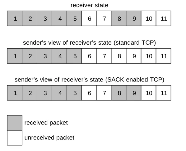
The SACK scheme adds extra information to acknowledgements about the receiver’s state each time TCP’s standard positive cumulative acknowledgement scheme is lacking. This happens when there are ‘gaps’ in the data the destination host has received. Standard TCP would acknowledge all data up to the first gap but TCP with SACK can effectively bridge a gap by sending an extra SACK block. By sending more information in acknowledgements the sender is better able to react to the actual state of the link and the receiver. The difference in supplied information to the sender is shown in the next figure.
Example 3.3. Consider the same situation as in Example 3.1. However, this time there is also a SACK enabled receiver. The receiver state and both the senders’ view of it are represented in the next figure.
1 2 3 4 5 6 7 8 9 10 11
1 2 3 4 5 6 7 8 9 10 11 sender’s view of receiver’s state (standard TCP)
receiver state
received packet
unreceived packet
1 2 3 4 5 6 7 8 9 10 11 sender’s view of receiver’s state (SACK enabled TCP)
Figure 3.3: Example based on the acknowledgement scheme of standard TCP and SACK enabled TCP.
18
The SACK scheme can include any number of SACK blocks up to a maximum of four. This is because there is a limit on the size of TCP headers. All TCP options (including SACK blocks) are included in a special TCP header field called TCP options. The more options a TCP implementation uses the less space there is left for SACK blocks. In general TCP implementations that include SACK support, there is enough space left for three SACK blocks.
Even though its headers are larger, a TCP implementation with SACK support generally has less data- and time overhead than a comparable implementation without SACK support, because it can handle retransmits more efficiently. Because of the less data- and time overhead SACK also performs better (in terms of throughput) than other protocols as was shown in [FAL96].
3.3.3 Delayed acknowledgements
In principle a TCP receiver should acknowledge each packet that it receives. So each packet that reaches its destination immediately triggers a 40 byte acknowledgement (sometimes it can be piggybacked on normal packets bound for the other host however). This can of course be considered as a waste of bandwidth. To remedy this the TCP standard allows for a receiver to delay the sending of an acknowledgement for a period of time (with a maximum of 500 milliseconds) [COM95]. In this way multiple acknowledgements can be combined and/or the acknowledgement(s) can be piggybacked on a normal data packet.
This of course reduces data overhead. Unfortunately there are also a few drawbacks. The first disadvantage is that the importance of an acknowledgement increases. That is, if such an acknowledgement is lost more information on the state of the receiver is lost than would be the case with a undelayed acknowledgement. Because more information is lost, the consequences can be more severe, possibly increasing data- and time overhead. The second drawback is that time overhead will probably increase because the receiver will not immediately send an acknowledgement but will wait for a period of time before doing so. This will cause the sender’s window to be built up more slowly.
Because TCP relies on acknowledgements to accurately estimate the round trip time, the sender is not allowed to combine too much acknowledgements. For every second data packet an acknowledgement should be sent, further reducing the decrease in data overhead.
19
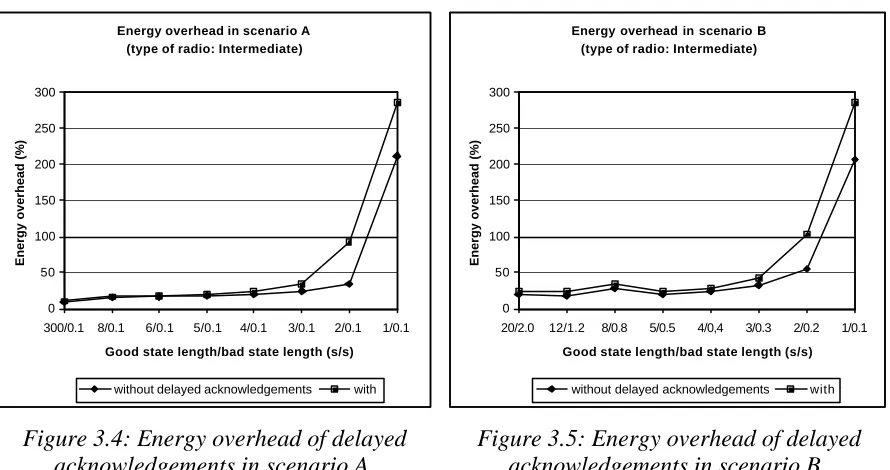
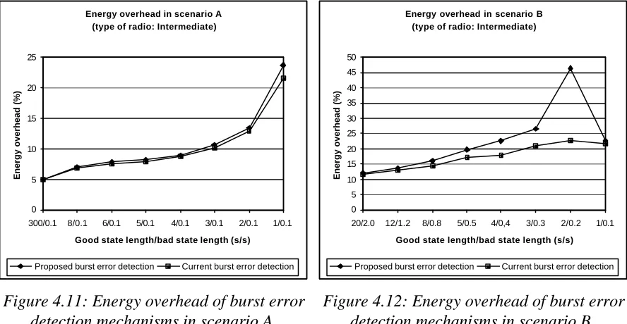
Energy overhead in scenario A (type of radio: Intermediate)
0 50 100 150 200 250 300
300/0.1 8/0.1 6/0.1 5/0.1 4/0.1 3/0.1 2/0.1 1/0.1
Good state length/bad state length (s/s)
Energy overhead (%)
without delayed acknowledgements with
Figure 3.4: Energy overhead of delayed acknowledgements in scenario A.
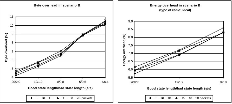
Energy overhead in scenario B (type of radio: Intermediate)
0 50 100 150 200 250 300
20/2.0 12/1.2 8/0.8 5/0.5 4/0,4 3/0.3 2/0.2 1/0.1
Good state length/bad state length (s/s)
Energy overhead (%)
without delayed acknowledgements with
Figure 3.5: Energy overhead of delayed acknowledgements in scenario B.
In both graphs it is quite clear that the use of delayed acknowledgements increases the energy overhead of a protocol and thus decreases its energy efficiency. From an energy efficiency standpoint, delayed acknowledgements should be avoided.
3.3.4 Explicit congestion notification
TCP’s flow control mechanisms rely on packet drops to detect congestion. When this happens TCP is already late in reacting because the congestion already occurred. It would be better if TCP could be notified when it is about to cause congestion so that it can react before packets are lost. Lost packets should be avoided because they will have to be retransmitted, increasing data (and time) overhead.
To improve TCP, an explicit congestion notification (ECN) system was proposed in RFC 2481 [RAM99]. In the proposed configuration both routers and end points should be ECN capable. When a router predicts that congestion will occur, it marks packets by setting a special ECN field in TCP packets. The receiver of the packet can then take appropriate measures to make sure the transmission rate of the connection will be reduced. In such a way congestion can often be avoided.
Although this scheme can decrease data- and time overhead (because less retransmits should be necessary) it is also possible it increases time overhead. When a TCP connection is incorrectly told to decrease its transmission rate for instance. Overall this scheme can decrease energy efficiency but is only suited for multi-hop paths. E2TCP will be used on a single-hop path. Thus it will not experience congestion on intermediate nodes, which is the reason there is no need to make use of explicit congestion notification in E2TCP.
3.3.5 Forward error correction
20
hand the processing power increases as well as the total size of the data that needs to be transmitted. This of course also results in increased transmission times.
ARQ schemes provide exactly as much error correction as is needed, because they only kick in when errors actually occur. The amount of error correction used in FEC schemes however, does not directly depend on the amount of errors that occurred. It in stead depends on the amount of expected errors and so the amount of FEC is decided upon in advance. Unfortunately predicting the future is still impossible, even for FEC schemes. So most of the time FEC schemes will either offer too much protection or too little. When too much protection is offered, too much data has been sent which means data- and time overhead could have been reduced. When too little protection was offered, the receiver could not correct the errors in the packet and the packet should be transmitted again. This is of course also the case when using an ARQ scheme but with the FEC scheme the packets are larger because of the added protection. So ARQ schemes can be said to be more energy efficient than FEC schemes [HAV99].
Furthermore using FEC in the transport layer is only possible when the lower layers also hand packets with errors to the transport layer. Because no assumptions were to be made about the lower layers FEC can not be used in E2TCP.
3.3.6 I-TCP
Indirect TCP [BAK95] is a solution specifically designed to be used with wireless connections. It was one of the first proposals to use split connections. The connections are named so because connections between the mobile host and fixed hosts are split up in two separate connections at the base station: one regular TCP connection between the base station and the fixed host and another connection between the mobile host and the base station. This last connection is a single-hop connection over a wireless link and there is no need to use standard TCP. Rather a more optimized wireless-link protocol can be used which solves some of TCP’s problems on wireless links. Another advantage of split connections is that it effectively separates the flow and congestion control at the base station. This way flow and congestion control on each sublink can be optimized separately from the other.
Indirect TCP largely refrains from changing the protocol on the wireless link and solely focuses on the split connection principle. Still this proposal is able to obtain impressive results [BAK97] and the split connection principle is very well suited for wireless access to a TCP/IP network.
3.3.7 Protocols inspired by I-TCP
The obvious advantages of the split connections approach inspired some other protocols. These protocols all use a (lightly) optimized version of TCP on the wireless links to further improve performance over I-TCP.
The Berkeley Snoop Module [BAL95] is another proposal to tackle the performance problems of TCP on wireless links. Just like I-TCP it proposes a split connection setup but the Snoop Module is more active than the I-TCP setup. The Snoop Module caches packets and performs local retransmissions as soon as packet loss is detected. This further increases performance over I-TCP.
21
In [RAT98] another protocol for networks with wireless links is proposed: WTCP. It closely resembles I-TCP but stresses the importance of accurate round trip time sampling and is constructed accordingly.
3.3.8 Delayed duplicate acknowledgements
The delayed duplicate acknowledgement scheme [VAI99] tries to mimic the behavior of the Snoop protocol but does it TCP-unaware, unlike the Snoop Module, which is TCP-aware. A TCP-aware protocol needs to look in the TCP headers in order to take appropriate measures. It is possible however that the TCP headers are not readable by intermediate hosts (because of encryption). This scheme tries to behave in the same way as the Snoop Module without examining the TCP headers. Because this scheme has less information to base its decisions on, it performs slightly worse than the Snoop Module. On the other hand it can be used in more situations.
3.3.9 Mobile-TCP
The Mobile-TCP protocol as described in [HAA97] is one of the few protocols that try to optimize for energy efficiency. It also employs the split connection principle but drastically changes the protocol on the wireless link. An asymmetric protocol is proposed: the protocol stack running at the mobile host is kept as small and simple as possible and as much processing is offloaded to the base station.
In order to save energy the protocol uses very small custom headers and makes use of the connection ID principle, known from header compression. The implementation at the mobile host also features as few timers as possible and the protocol does not use the sliding windows principle, allowing for smaller buffers. Furthermore, the protocol for instance, does not support flow control or resequencing.
Overall this protocol sacrifices so much in order to save on processing power, it will undoubtedly spend more energy on retransmits than other (energy efficient) protocols. Because the relative power consumption of processors, compared to radios, keeps decreasing, it is not that interesting to focus on minimizing required processing power. Minimizing data- and time overhead seems a better way to increase energy efficiency.
3.3.10 PRTP
The partial reliable transport protocol (PRTP) [BRU00] was not specifically designed with wireless links in mind but with a type of traffic. The strict reliability guarantees of TCP make it less suited for many multimedia applications. Often when streaming media experiences small amounts of data loss, retransmission is actually undesirable. They cause the playback to stall and the retransmitted data will already have ‘expired’ upon arrival. Furthermore most streaming media can withstand small amounts of data loss without a noticeable loss in quality. For such connections the partial reliability transport protocol, which is compatible with TCP, offers a solution.
22
In case of packet loss PRTP performs very well compared to other versions of TCP. Please note that this does mean that the PRTP receiver receives not all data. Because wireless links generally experience much packet drops, PRTP is extremely well suited for streaming media over wireless links.
3.3.11 Optimized window management
One might think that this concept does not deserve it’s own paragraph. However, the way in which TCP reacts to (burst) errors on wireless links leaves a lot to be desired. Every packet loss is considered to be caused by congestion. For each packet loss TCP will drastically reduce its transmission speed so experienced congestion will quickly be cleared. The assumption that each packet loss is caused by congestion is valid in wired networks. Because of the high reliability of such links, the largest portion of packet loss is indeed caused by congestion. However, on wireless links, the assumption is not valid. Because of the relatively low channel quality of wireless links, a lot of packets will be corrupted while in transit. For each of those errors TCP will also reduce its transmission speed. A huge loss in time overhead can therefor be reached by optimizing the window management scheme of a protocol for wireless links.
3.3.12 Conclusions
Some of the concepts and protocols presented in this chapter are not applicable when optimizing for energy efficiency. They either focus on ways to improve performance that do not increase energy efficiency or they optimize the power consumption of the wrong part of the system. The other concepts presented here will be used in order to design a energy-efficient transport protocol and these include:
• split connections
• small headers
• selective acknowledgements
• partial reliability
23
4
E
2TCP
In this chapter, E2TCP will be described in detail. First an overview of the architecture of E2TCP will be given, where the reasons for and expectations of the changes to TCP will be discussed. After that, the header format will be explained in detail, followed by the selective acknowledgement scheme. Finally, the window management will be described, as well as the partial reliability mechanism.
4.1
Architecture overview
One of the primary goals of this project was to design a transport protocol that would be compatible with TCP. It was therefore only self-evident that TCP would serve as a basis for this new protocol. Because E2TCP is derived of TCP, its architecture and mechanisms are roughly the same. On four points, however, adjustments were made to increase the energy efficiency of the protocol. These points are the headers, the acknowledgements, the window management and the reliability requirements. All four changes will be introduced in the following paragraphs.
4.1.1 Headers
The large header size of TCP was first introduced as a problem in Paragraph 3.2.1. The unnecessarily large headers are the cause of equally-unnecessary data overhead. The custom headers of E2TCP are the result of a rather straightforward implementation of some of the ideas of header compression standards, presented in Paragraph 3.3.1. The main principle that was used was: if it is not necessary to transmit a certain header field, don’t do it. This principle is so self-evident; one could wonder why such a system was not incorporated in the TCP standard.
All header fields of TCP/IP datagrams were analyzed whether they should be included in the headers of E2TCP at all, whether they should always be sent or whether they were to be made optional. Such an optional header field will then only be sent if it is necessary to do so. Care was taken to keep the headers robust because the problems of a non-robust compressed header system, explained in Example 3.2, have to be avoided.
The header size is reduced from 40 bytes to 8 bytes (in most situations). When using 1000 byte packets for instance, the data overhead introduced by the headers of E2TCP will be 1.6% as opposed to 8.0% for the headers of standard TCP. Because less data has to be transmitted, the time overhead will probably also decrease somewhat, although perhaps not as much as the data overhead. This will probably result in a decrease in energy overhead of about 5%. The details of the headers of E2TCP will be discussed in Paragraph 4.2.
4.1.2 Acknowledgements
The simple acknowledgement scheme of TCP, introduced as a problem in Paragraph 3.2.2, is another point of TCP that could be improved to increase energy efficiency. In case of missing packets the sender simply has not enough information about the state of the receiver. On those occasions, it is possible the sender not always decides on the optimal course of action. A solution to this problem is the use of selective acknowledgements, which were introduced in Paragraph 3.3.2.
24
packets. When the sender receives such an acknowledgement it is always able to choose the most energy efficient course of action. Because of the diminishing returns of adding more SACK blocks and the fact that SACK blocks increase the size of the acknowledgements, a maximum of two SACK blocks is used.
Although SACK blocks increase data overhead because the acknowledgements increase in size when these blocks are used, the effect of selective acknowledgements on the energy efficiency will be positive. This is because the sender is able to react in an optimal way to lost packets, which slightly decreases data overhead (because of less retransmits) and reduces time overhead substantially (because of a better utilization of the available bandwidth). However, giving an exact estimate of the increase in energy efficiency is impossible. The implementation of selective acknowledgements in E2TCP will be explained in detail in Paragraph 4.3.
4.1.3 Window management
The problems of TCP on wireless links with respect to its window management were introduced in Paragraph 3.2.3. The assumption of TCP that each packet loss is an indication of congestion is valid on wired networks, but has little value on wireless links. This is because the inherent unreliability of wireless networks, which causes a substantial amount of packets to be lost because of errors on the link itself. So, the window management of TCP should be altered to include (burst) errors as a possible source of packet loss, as was indicated in Paragraph 3.3.11.
The window management mechanism of E2TCP differs on four points from that of TCP. First of all, E2TCP features immediate retransmits. When the receiver indicates it has received an out-of-order packet, the sender can immediately retransmit the missing packets, because E2TCP will be used on a single-hop link and no packet reordering can take place on such a link. Under the same conditions TCP would wait on a timeout before it would retransmit the lost packet, causing substantial delays. This change will therefore primarily decrease the time overhead.
The second change is that E2TCP reacts to (burst) errors in a different way. If few errors occur, E2TCP considers this to be the result of normal static and barely reduces its transmission speed. When lots of errors occur, E2TCP considers a burst error to be the cause and drastically reduces its transmission speed. This way, E2TCP reacts to (burst) errors in a very energy efficient way, as will be shown in Paragraph 5.6. It should be noted that this new window management scheme relies on selective acknowledgements to detect the number of errors. Both data and time overhead will decrease because of this change.
E2TCP also features a minimum window size, which is the third point on which the window management of TCP and E2TCP differ. This minimum window size causes E2TCP to quickly recuperate after a burst error, which will decrease time overhead.
25
4.1.4 Reliability requirements
Because the strict reliability requirements of a TCP connection are not always desirable, as was shown in Paragraph 3.2.4, the concept of partial reliability was developed, which was introduced in Paragraph 3.3.10. When transmitting streaming media, energy can be saved if unwanted retransmits can be avoided. Partial reliability provides a way to do this, by enabling the application to set the minimum desired reliability of the channel.
The implementation of partial reliability in E2TCP is rather straightforward. The receiver keeps track of how much data was successfully received and how much was lost. If it detects packet loss it will check if the actual reliability still exceeds the minimum desired reliability and if so, will simply acknowledge the lost packet. The sender will think it was received correctly and will refrain from retransmitting.
This simple mechanism will be able to decrease the energy overhead. How much is uncertain but its effect will increase when channel conditions deteriorate. This is because the effect of stopping retransmits increases when more packets are lost. The details of the implementation will be discussed in Paragraph 4.4.6.
4.2
Header format
The headers of E2TCP packets will be explained in this paragraph. Because E2TCP needs to be compatible with TCP/IP, the headers of IP and TCP will be examined first. Based on that information, a decision can be made on what header fields should be included in E2TCP headers, which will be explained in Paragraph 4.2.3.
4.2.1 IP header
The Internet calls its basic transfer unit an (IP) datagram. Such a datagram is divided into a header (of 20 bytes) and a data area in the following way:
header user data
IP datagram
Figure 4.1: An IP datagram.
According to [DEG99], all fields in headers can be classified into one of the following four categories depending on how they are expected to change between consecutive headers in a packet stream. These four categories are:
• Inferred: The field contains a value that can be inferred from other values, and thus need not be transmitted.
• Nochange: The field is not expected to change during the packet stream. Such a value only has to be transmitted once.
• Delta: The field may change often but usually the difference from the field in the previous header is small, so that is more efficient to send the deviation from the previous value rather than the current value.
• Random: The field changes unpredictably and should therefore probably be sent in full.
26
VERS HLEN SERVICE TYPE TOTAL LENGTH
HEADER CHECKSUM IDENTIFICATION
SOURCE IP ADDRESS
DESTINATION IP ADDRESS TIME TO LIVE PROTOCOL
FRAGMENT OFFSET FLAGS
0 4 8 16 19 24 31
Figure 4.2: The IP header format.
The header fields of an IP datagram are:
Field Type Description
Protocol version (VERS)
nochange This field contains the version of the IP protocol that was used to create the datagram and is of course not expected to change within a packet stream. On the wireless link, E2TCP will operate and it does not need to know which version of TCP is used on the wired part of the connection. Therefore this field can be omitted from the E2TCP header.
Header length (HLEN)
inferred This field contains the length of the header but this can be determined by other means as well, so there is no need to include it in the header of an E2TCP packet.
Service type nochange With this field the sender can specify the type of transport desired. It is, however, often ignored by hosts and routers and is not expected to change. E2TCP does not support different types of services and it does not need to include this field in its headers.
Total length inferred This field contains the length of the complete datagram but that will also be specified by any reasonable link-level protocol. It is unnecessary to include it in E2TCP headers.
Identification random For each datagram a unique number is stored in this field. It is used to refragment split up datagrams. On a point-to-point link (where E2TCP will operate) no fragmentation will take place and each packet will be identified by its sequence number or acknowledgement number (TCP header fields).
Flags random These flags control the fragmentation of the datagram and can be left out of the header.
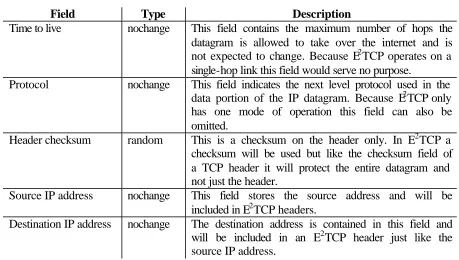
27
Field Type Description
Time to live nochange This field contains the maximum number of hops the datagram is allowed to take over the internet and is not expected to change. Because E2TCP operates on a single-hop link this field would serve no purpose.
Protocol nochange This field indicates the next level protocol used in the data portion of the IP datagram. Because E2TCP only has one mode of operation this field can also be omitted.
Header checksum random This is a checksum on the header only. In E2TCP a checksum will be used but like the checksum field of a TCP header it will protect the entire datagram and not just the header.
Source IP address nochange This field stores the source address and will be included in E2TCP headers.
Destination IP address nochange The destination address is contained in this field and will be included in an E2TCP header just like the source IP address.
Table 4.1: The IP header fields.
IP also allows some optional extra information to be sent in its headers. Timestamps and source routes are among them. As said these fields are optional and need not be supported by E2TCP. Furthermore the base station can still support most of them, so these options can be used on the wired path of the connection.
Of all these header fields only three will be included (in one way or another) in the E2TCP header: the source- and destination IP address and the checksum.
4.2.2 TCP header
A TCP packet is encapsulated in an IP datagram and is divided into a header (of 20 bytes) and payload in a way similar to an IP datagram.
IP header user data: TCP datagram
IP datagram
user data TCP header
TCP datagram
Figure 4.3: A TCP datagram within an IP datagram.
28
DESTINATION PORT
WINDOW
CHECKSUM
SEQUENCE NUMBER
ACKNOWLEDGEMENT NUMBER
HLEN RESERVED
0 4 10 16 24 31
SOURCE PORT
CODE BITS
URGENT POINTER
Figure 4.4: The TCP header format.
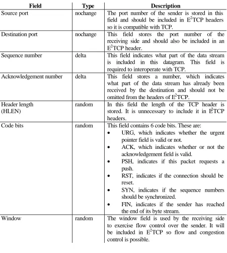
The fields of a TCP header are:
Field Type Description
Source port nochange The port number of the sender is stored in this field and should be included in E2TCP headers so it is compatible with TCP.
Destination port nochange This field stores the port number of the receiving side and should also be included in an E2TCP header.
Sequence number delta This field indicates what part of the data stream is included in this datagram. This field is required to interoperate with TCP.
Acknowledgement number delta This field stores a number, which indicates what part of the data stream has already been received by the destination and should not be omitted from the headers of E2TCP.
Header length (HLEN)
random In this field the length of the TCP header is stored. It is unnecessary to include it in E2TCP headers.
Code bits random This field contains 6 code bits. These are:
• URG, which indicates whether the urgent pointer field is valid or not.
• ACK, which indicates whether or not the acknowledgement field is valid.
• PSH, indicates if this packet requests a push.
• RST, indicates if the connection should be reset.
• SYN, indicates if the sequence numbers should be synchronized.
• FIN, indicates if the sender has reached the end of its byte stream.
29
Field Type Description
Checksum random As indicated in the previous paragraph, a checksum will be included in the E2TCP headers, which will protect the entire E2TCP datagram.
Urgent pointer random This field indicates which data in the packet is of a special urgent type, which deserves special treatment from the receiver. In order to interoperate with TCP, this field will be included in the headers.
Table 4.2: The TCP header fields.
TCP also allows some optional extra information to be sent in TCP headers. Timestamps and SACK blocks are among them. As said these fields are optional and need not be supported by E2TCP. Furthermore the base station can still support most of them, so these options can be used on the wired path of the connection.
Of all these header fields the following will be used in E2TCP headers: source- and destination port numbers, sequence and acknowledgement numbers, window, urgent pointer and, as already said, the checksum.
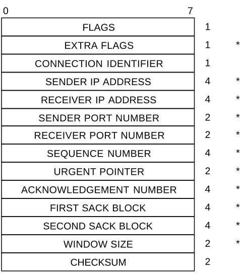
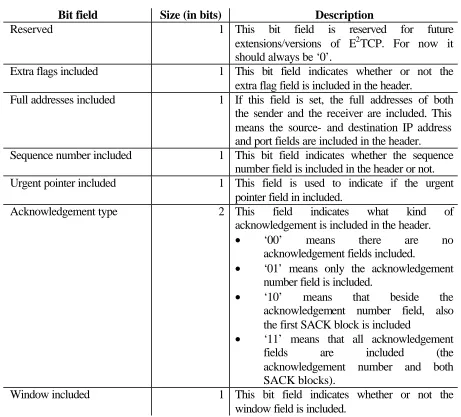
4.2.3 E2TCP header
To get an overview of the fields that were chosen to be included in the headers of E2TCP, they will be listed again with their type and size.
Field Type Size (in bytes)
Source IP address nochange 4
Destination IP address nochange 4
Source port number nochange 2
Destination port number nochange 2
Sequence number delta 4
Acknowledgement number delta 4
Window random 2
Urgent pointer random 2
Checksum random 2
Table 4.3: The E2TCP header fields.
But that is not all info