EM-Based Channel Estimation Algorithms for OFDM
Xiaoqiang Ma
Department of Electrical Engineering, School of Engineering and Applied Science, Princeton University, Princeton, NJ 08544-5263, USA
Email:[email protected]
Hisashi Kobayashi
Department of Electrical Engineering, School of Engineering and Applied Science, Princeton University, Princeton, NJ 08544-5263, USA
Email:[email protected]
Stuart C. Schwartz
Department of Electrical Engineering, School of Engineering and Applied Science, Princeton University, Princeton, NJ 08544-5263, USA
Email:[email protected]
Received 26 February 2003; Revised 16 September 2003
Estimating a channel that is subject to frequency-selective Rayleigh fading is a challenging problem in an orthogonal frequency di-vision multiplexing (OFDM) system. We propose three EM-based algorithms to efficiently estimate the channel impulse response (CIR) or channel frequency response of such a system operating on a channel with multipath fading and additive white Gaussian noise (AWGN). These algorithms are capable of improving the channel estimate by making use of a modest number of pilot tones or using the channel estimate of the previous frame to obtain the initial estimate for the iterative procedure. Simulation results show that the bit error rate (BER) as well as the mean square error (MSE) of the channel can be significantly reduced by these algorithms. We present simulation results to compare these algorithms on the basis of their performance and rate of convergence. We also derive Cramer-Rao-like lower bounds for the unbiased channel estimate, which can be achieved via these EM-based algo-rithms. It is shown that the convergence rate of two of the algorithms is independent of the length of the multipath spread. One of them also converges most rapidly and has the smallest overall computational burden.
Keywords and phrases:OFDM, EM-algorithm, channel estimation, Cramer-Rao lower bound.
1. INTRODUCTION
Orthogonal frequency division multiplexing (OFDM) [1], a spectrally efficient form of frequency division multiplex-ing (FDM), divides its allocated channel spectrum into sev-eral parallel subchannels. OFDM is inherently robust against frequency-selective fading since each subchannel occupies a relatively narrowband, where the channel frequency char-acteristic is nearly flat. OFDM has an additional advan-tage of being computationally efficient because the fast Fourier transform (FFT) technique can be used to imple-ment the modulation and demodulation functions [2]. Fur-thermore, the OFDM system can eliminate interframe in-terference (IFI1) through the use of a cyclic prefix (CP)
that is longer than the order of the channel impulse
re-1In the literature, the term intersymbol interference (ISI) is used, but we believe IFI is more appropriate in this paper.
sponse (CIR). OFDM has already been used in European digital audio broadcasting (DAB), digital video broadcasting (DVB) systems, high performance radio local area network (HIPERLAN) and IEEE 802.11a wireless local area networks (WLAN). It has also been shown that OFDM is an effective way of increasing data rates and simplifying the equalization in wireless communications [3].
Input
bits Modulation Modulated signalsX(m)
S/P ... IFFT ... Add cyclic prefix
. . . P/S
Transmitter
Channel
Output
bits Demodulation Estimated signals ˆX(m)
One-tap EQ & P/S
. .
. FFT ...
Remove cyclic prefix
. . . S/P
Channel estimation
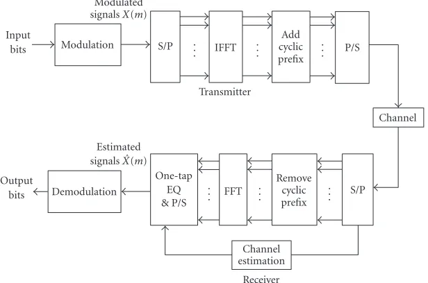
Receiver Figure1: Baseband OFDM system model.
such pilot-assisted estimation algorithms adopt an interpola-tion technique with fixed parameters (two-dimensional (2D) [6,7] or one-dimensional (1D) [5]) to estimate the channel frequency response by using the channel estimate obtained at the lattices assigned to the pilot tones. Linear, spline, and Gaussian filters have all been studied [5]. Another method in this category adopts a known channel frequency covari-ance matrix and uses a channel estimate at pilot tones to estimate the CIR in the sense of minimum mean square error (MMSE) [4, 8, 9, 11]. Shortcomings of these algo-rithms include (1) a large error floor that may be incurred by a mismatch between the estimated and real CIR, (2) dif-ficulty in obtaining the channel frequency covariance matrix and the resultant error due to channel statistics mismatch, and (3) spectrum inefficiency due to the overhead (typi-cally 20%) associated with use of pilot symbols. In addition, several kinds of blind channel estimation algorithms have been proposed in order to improve transmission efficiency. These algorithms are based on the statistical property of re-ceived signals (e.g., second-order statistics [12,13,14,15]), the characteristic of virtual subcarriers [16], and the finite-alphabet property of transmitted signals [18]. However, each of these blind estimation algorithm has its limitation. For example, second-order statistics-based algorithms cannot be used in a high mobility environment (i.e., a large Doppler spread) since they require many blocks of data to carry out the estimation procedure. A finite-alphabet-based algorithm can be applied only to a constant modulus signal. In con-trast, in this paper, we extend and enhance some existing pilot-based channel estimation algorithms by substantially reducing the number of pilot symbols using the expectation-maximization (EM) algorithm.
The EM algorithm [19, 20] is a technique for finding maximum likelihood (ML) estimates of system parameters in a broad range of problems where observed data are in-complete. The EM algorithm consists of two iterative steps:
the expectation (E) step and the maximization (M) step. The E-step is performed with respect to the unknown underlying parameters, using current estimates of the parameters, con-ditioned upon the incomplete observations. The M-step then provides new estimates of the parameters that maximize the expectation of the log-likelihood function defined over com-plete data, conditioned on the most recent observation and the last estimate. These two steps are iterated until the esti-mated values converge.
The main objective of this paper is to investigate the use of the EM algorithm for channel estimation of an OFDM sys-tem that is subject to slow time-varying frequency-selective fading. Three different algorithms have been developed and compared. In each of the algorithms, the initial channel esti-mate is obtained either from pilot symbols (that are inserted in the OFDM frame) or from the channel estimate of the pre-vious OFDM frame (where there is no pilot symbol in the current OFDM frame).
The rest of the paper is organized as follows. InSection 2, we will describe the baseband OFDM system model and dis-cuss some assumptions. InSection 3, the three different EM-based channel estimation algorithms are derived and fully discussed. The Cramer-Rao lower bound (CRLB) and mod-ified CRLB (MCRB) are discussed inSection 4for both con-stant and nonconcon-stant modulus signals. Comprehensive sim-ulation results and discussion are given inSection 5. Finally, we draw some conclusions inSection 6.
2. SYSTEM MODEL AND ASSUMPTIONS
The schematic diagram (Figure 1) is a baseband equivalent representation of an OFDM system. The input binary bits2
are first fed into a serial-to-parallel (S/P) converter. Each
data stream then modulates the corresponding subcarrier by MPSK or MQAM. The modulation scheme may vary from one subcarrier to another in order to achieve the maximum capacity or the minimum bit error rate (BER) for a given channel characteristic and total signal power constraint. In this paper, we assume, for simplicity, that only QPSK or 16 QAM is used in any of these subcarriers. We useM to de-note the number of subcarriers in the OFDM system. The modulated data symbols, represented by complex variables
X(0),. . .,X(M−1), are then transformed by the inverse fast
Fourier transform (IFFT). The output symbols are denoted
asx(0),. . .,x(M−1) and are given by
x(k)=√1
M
M−1
m=0
X(m)ej2π(km/M), 0≤k≤M−1. (1)
In order to avoid IFI, CP symbols, which replicate the end part of the IFFT output symbols, are added in front of each frame, that is,
x(k)=x(M+k), −Ncp≤k≤ −1, (2)
where Ncp denotes the length of the CP. The parallel
data are converted back to a serial data stream, that is,
x(M −Ncp),. . .,x(M −1),x(0),. . .,x(M −1), and
trans-mitted over the frequency-selective channel with addi-tive white Gaussian noise (AWGN). The received data
y(−Ncp),. . .,y(−1),y(0),. . .,y(M−1) are converted back
to Y(0),. . .,Y(M−1) after discarding the prefix symbols
y(−Ncp),. . .,y(−1), and applying the FFT and
demodula-tion to the remaindery(0),. . .,y(M−1).
The channel model we adopt in the present paper is a multipath slowly time-varying (unchanged in any one OFDM frame) fading channel, which can be described by
y(k)=
L−1
l=0
hlx(k−l) +n(k), 0≤k≤M−1. (3)
The CIRhl’s (0≤l≤L−1) are independent complex-valued
Gaussian random variables (which represents a frequency-selective Rayleigh fading channel), and n(k)’s (0 ≤ k ≤ M−1) are i.i.d. complex-valued Gaussian random variables with zero mean and varianceσ2for both real and imaginary
components.Lis the length of the CIR.
If we add the CP in each OFDM data frame, with its length chosen to be longer thanL, there will be no IFI be-tween OFDM frames. Thus, we only need to consider one OFDM frame at a time in deriving the system model. After discarding the CP and performing an FFT at the receiver, we can obtain the received data frame in the frequency domain:
Y(m)=√1
M
M−1
k=0
y(k)e−j2π(km/M), 0≤m≤M−1. (4)
Then using the CP condition (2), we obtain the following simple expression:
Y(m)=X(m)H(m) +N(m), 0≤m≤M−1, (5)
whereH(m) is the frequency response of the channel at sub-carriermdefined as follows:
H(m)=
L−1
l=0
hle−j2π(ml/M), 0≤m≤M−1, (6)
and the set of the transformed noise variables N(m), 0 ≤
m≤M−1,
N(m)=√1
M
M−1
k=0
n(k)e−j2π(mk/M), 0≤m≤M−1, (7)
are i.i.d. complex-valued Gaussian variables and have the same distribution asn(k), that is, with mean zero and vari-anceσ2. In a regular OFDM system, the channel delay spread L is much smaller than the number of subcarriers. This leads to a high correlation between the channel frequency re-sponsesH(m), 0≤m≤M−1, even whenhl, 0≤l≤L−1,
are independent.
In this paper, we assume the CIR is constant in each OFDM frame and varies from frame to frame according to the fading rate. However, in the derivation below, we assume, for generality, that the channel is constant duringDOFDM frames. Note that intercarrier interference (ICI) is also elim-inated at the FFT output because of the orthogonality be-tween the subcarriers under the assumption that the CP is longer than the channel delay spread. Furthermore, we as-sume the system has perfect timing and frequency synchro-nization.
Notation
We use the standard notation, that is, (·)Tdenotes the
trans-pose, (·)∗denotes the complex conjugate, (·)Hdenotes the
Hermitian, underscore letters stand for column vectors, and bold letters stand for matrices. We denote the pth estimates of the channel response in the frequency domain asH(p)and
in the time domain ash(p), and transmitted signals asX(p).
3. EM-BASED CHANNEL ESTIMATION ALGORITHMS
3.1. Introduction to the EM algorithm
The EM algorithm [19,20] is an iterative method to find the ML estimates of parameters in the presence of unobserved data. The idea behind the algorithm is to augment the ob-served data with latent data, which can be either missing data or parameter values, so that the likelihood function condi-tioned on the data and the latent data has a form that is easy to manipulate. The algorithm can be broken down into two steps: the E-step and the M-step. We assume that the data Z(“complete” data) can be separated into two components, Z = (X,Y), whereXare the observed data (“incomplete” data) and Yare the missing data. We denote θ as the un-known parameter we try to estimate fromY.
The E-step findsQ(θ|θ(p)), the expected value of the
ofθ,θ(p):
This procedure is repeated until the sequenceθ(0),θ(1),
θ(2),. . .converges. The EM algorithm is constructed in such
a way that the sequence ofθ(p)’s converges to the ML estimate
ofθ.
Applications of the EM algorithm to estimation problems in communications systems have appeared a lot in the liter-ature. Channel estimation [21] and signal detection [22,23] are two typical applications of the EM algorithm. Georghi-ades and Han [22] provide a general study of data sequence estimation in the presence of random parameters. Zeger and Kobayashi [23] give a simplified algorithm to detect contin-uous phase modulated signals in fading channels. In the re-mainder of this section, we propose three different EM-based channel estimation and signal detection algorithms by defin-ing different “complete” and “incomplete” data sets for these algorithms.
3.2. Algorithm 1: estimating the channel frequency response
OFDM divides its allocated channel spectrum into several parallel subchannels that are only subjected to frequency flat fading. Thus, we only need to estimate the individualH(m), 0≤m≤M−1, separately, which will result in a considerable reduction in computational complexity. To simplify the ex-pressions, we omit the subcarrier indexm, and simply write Y,X, andHinstead ofY(m),X(m), andH(m).
We assume that the frequency-domain signalXof a given subcarrier represents a QPSK or 16 QAM signal with constel-lation sizeC(=4 or 16, respectively). We denote the symbols in the signal constellation by{Xi, 1≤i≤C}.
Due to the Gaussian noise assumption, the probability density function (pdf) ofYgivenXandHis given by
f(Y|X,H)= 1
By assuming that allCsymbols are equally likely and averag-ing the conditional pdf of (10) over the variableX, we obtain the pdf ofYgivenHas follows:
f(Y|H)=
Suppose the channel is static over the period ofDOFDM frames. Different values ofDcan be applied in different ap-plications depending on how rapidly the channel changes. We define the received signal vectorY = [Y1,. . .,YD] and
the transmitted signal vectorX=[X1,. . .,XD] for a specific
subcarrier overDframes. Then we callYand (Y,X) “incom-plete” and “com“incom-plete” data, respectively, following the termi-nology of the EM algorithm. Assuming that additive Gaus-sian noise is independent from frame to frame for each sub-carrier, we can write the conditional pdf of the incomplete data as follows:
f(Y|H,X)=
D
d=1
fYdH,Xd. (12)
Thus, the log-likelihood function of the incomplete data is
logf(Y|H,X)=
D
d=1
logfYdH,Xd, (13)
and the log-likelihood function of the complete data is given by
In the conventional ML estimation, we try to find an es-timate ofH that maximizes f(Y|H). But since logf(Y|H), (11), is not easy to manipulate (summation of several ex-ponential functions), we resort to the EM algorithm, which increases the likelihood at each step. Each iterative process p=0, 1, 2,. . .in the EM algorithm for estimatingHfromY consists of the following two steps:
E-step:
where (seeAppendix A)
QHH(p)=
through additional manipulation on ˜H(p+1). The conditional
pdfs f(Yd|H(p),X
i) and f(Yd|H(p)) can be calculated from
(10) and (11), whereXiis theith signal in the constellation.
The value of H that maximize (17) is found as (see Appendix B) follows:
˜
˜ Figure2: Lowpass filter structure.
In this paper, we assume thatL, the delay spread in the CIR, is known. In practice, however,Lis another unknown parameter. In such a case, we need to perform channel-order detection and parameter estimation. Alternatively, we may use some upper bound forL, which may be easier to obtain than trying to estimate the exact value ofL. However, use of an upper bound ofLwould degrade the estimation perfor-mance. One obvious upper bound ofLcan be the length of the CP since its length is chosen to be longer thanL.
The channel estimate of the form (18) obtained for theM subcarriers, which we denote ˜H(p+1)(m), 0≤m≤M−1, can
be refined by taking advantage of the structure of OFDM sys-tems and the fact thatLis much smaller thanM, the number of subcarriers. We will proceed as follows:
h(p+1)= 1
where we use the notation defined inSection 3.3for mathe-matical simplification andWLis anM×Lmatrix:
WL=
Finally, we can obtain the (p+1)st estimate of the channel frequency response as follows:
H(p+1)=WLh(p+1). (21)
The above procedure can be simply realized by applying the IFFT followed by the FFT, as schematically shown inFigure 2. The valuesh(lp+1),L≤l≤M−1, obtained by the IFFT must
be set to zero before performing the FFT. The reason is to eliminate the estimation noise from paths that do not actu-ally exist.
The iterative procedure should be terminated as soon as the difference betweenH(p+1)andH(p)is sufficiently small, since at this point,H(p)has presumably converged to the
esti-mate we are seeking. Once the frequency-domain channel re-sponse ˆHis found, the ML estimate of the transmitted signal
can be obtained by solving
ˆ which leads to the final estimates of the transmitted signals as follows:
For a constant modulus signal, for example, a PSK mod-ulation signal|X(m)|2 = Afor allm, whereAis a positive
constant. Thus, we can simplify (18) as follows:
˜
Notice that only the noise varianceσ2 is used to
calcu-late f(Yd|H(p),X
i) in this algorithm. Any other statistical
in-formation about the channel is not necessary. Moreover, in Section 5, we will show that the accuracy ofσ2will not affect
the performance very much. Thus, this algorithm is fairly ro-bust to the noise variance.
3.3. Algorithm 2: estimating the transmitted signals
In this algorithm, we try to improve the performance of the detection accuracy of the transmitted signalXd(m), 0≤m≤
M−1, 1≤d≤D, as well as the CIR from the observation Yd(m), 0 ≤ m ≤ M−1, 1 ≤ d ≤ D, using the EM
algo-rithm. To simplify the expressions, we useH,h,X,Y,Nto denote the vectors of frequency-domain CIR, time-domain CIR, modulated input data, output data, and white Gaus-sian noise, respectively, where h = [h0,. . .,hL−1]T,Xd = system model can be expressed in the vector form for thedth OFDM frame as follows:
Yd=XdW
Lh+Nd. (25)
We still assume that the channel is static over the pe-riod of D frames for generality. To process the chan-nel estimation algorithm using observed data in all D frames, we define some variables:X=[(X1)T,. . ., (XD)T]T,
Y = [(Y1)T,. . ., (YD)T]T,N = [(N1)T,. . ., (ND)T]T,X =
diag(X),Y = diag(Y), andWLD = [WL,. . .,WL]T withD
copies ofWL. With this notation, the system model can be
modified as follows:
Y=XWLDh+N. (26)
E-step:
In the E-step at the (p+ 1)st iteration, we compute the ex-pected value of logf(Y,h|X), givenYandX(p), the estimates
obtained in thepth iteration. The M-step of the (p+ 1)st it-eration determines the transmitted signalX(p+1)that
maxi-mizesQ(X|X(p)) givenX(p).
After some calculations (seeAppendix C), we obtain the solution of (28): posterior covariance matrix at thepth iteration. Therefore, in each iteration, the updated estimation of CIRh(p)is obtained automatically as a by-product. After quantizing ˜X(p+1), we obtain the (p+ 1)st estimate
X(p+1)=QuantizationX˜(p+1). (35)
The limitation of this algorithm is that the meanE{h}
and the covariance matrixΣof time-domain CIR are also as-sumed to be known. In a practical situation, these channel statistics may not be known. Fortunately, as we examine (33) and (34), we find that whenσ2is small (i.e., SNR is high),
the contribution ofΣ−1andΣ−1E{h}is so small that we can eliminate them and still expect similar performance. Further-more, for an MPSK modulated signal, that is,|X(m)|2 =A
for allm, the signal estimation can be performed by using only the phase information. Thus, we can simplify (35) to
X(p+1)=QuantizationYHX(p)W
LDWHLDY
T
. (36)
Consequently, only multiplication and addition operations are required. Furthermore,WLDWHLDcan be calculated and
stored ahead of time. Thus, the computational complexity is considerably reduced for the high SNR case.
A closer examination of (36) reveals that the simplified Algorithm 2 is a combination of ML channel estimation as-sumingX(p)=Xand ML signal detection assumingh(p)=h. This has been proposed in [17] in a different context. To conclude, Algorithm 2 is the extension of the iterative ML channel estimation algorithm when we take advantage of the channel statistics. The corresponding simplified algorithm is the same as the iterative ML channel estimation algorithm.
3.4. Algorithm 3: estimating the channel impulse response
In this section, we try to estimate the time-domain chan-nel response by applying the parameter estimation algorithm proposed by Feder and Weinstein [24] for the general esti-mation problem based on the EM algorithm. We still assume that the channel is static over the period ofDframes for gen-erality. The system model used here is the same as the previ-ous algorithm stated in (26). We defineA=XWLDwhich is
aMD×Lmatrix, and rewrite the system model as follows:
Y =Ah+N=
L−1
i=0
Aihi+N, (37)
whereAiis theith column of the matrixA. Note from (37)
that each element of Y,Y(m), consists of Lsuperimposed signals and AWGN which can be represented by
Y(m)=
L−1
i=0
ai(m)hi+N(m), 0≤m≤MD−1. (38)
Following [24], a natural choice for the “complete” dataZm
is defined by decomposing the observed data Y(m) into L components, that is,Zm=[Z0(m),. . .,ZL−1(m)]T, where
Zi(m)=ai(m)hi+Ni(m), 0≤m≤MD−1. (39)
Here,ai(m) is the (m,i)th entry of the matrixAandNi(m),
0 ≤i≤L−1, are obtained by arbitrarily decomposing the total noiseN(m) intoLcomponents such that
L−1
i=0
Ni(m)=N(m). (40)
Thus, the relation between the “complete” dataZmand
“in-complete” dataY(m) is given by
Y(m)=
L−1
i=0
Zi(m). (41)
It is convenient to choose the Ni(m) to be statistically
in-dependent Gaussian random variables with zero mean and varianceσi2, where
“complete” data formth element ofY, as stated before, are (Y(m)) and (Zm), respectively. We then group allZmfor all
D OFDM frames and all M subcarriers into a new vector
Z =[ZT0,. . .,ZTMD−1]T. Each iterative processp =0, 1, 2,. . .
in the EM algorithm for estimatinghfromYconsists of the following two steps:
In the E-step at the (p+1)st iteration, we compute the ex-pected log-likelihood function logf(Z|h), givenYandh(p), the estimates obtained in thepth iteration. The M-step of the (p+ 1)st iteration determines the transmitted CIRh(p+1)that maximizesQ(Z|h(p)).
After some calculation (seeAppendix D), we obtain the solution of (44):
Observe thatβi, theith decomposition factor, can be
ar-bitrarily selected with the constraint (47) due to the arbitrary selection of the independent noise componentsNi(m).
Dif-ferent sets of βi will give different system performance and
we will discuss the selection ofβiwith simulation results in
the next section.
Note that the elements ofA=XWLD are dependent on
the transmitted signalsX. However, we do not know all these transmitted signals in the OFDM frames except for some pi-lot symbols. Thus, in order to proceed, we adopt thepth esti-matesX(p)instead of the actual values (which are unknown) to calculate the matrixA. In this case, the elements ofX(p)
Notice that we do not need any information about the channel in this algorithm except the choice of the setβi.
How-ever, we can always chooseβi=1/Lwhich will give near
opti-mum performance as demonstrated in the simulation results. Thus, this algorithm is also very robust.
3.5. Initialization
As is known from the general convergence property of the EM algorithm, there is no guarantee that the iterative steps converge to the global maximum. For a likelihood function with multiple local maxima, the convergence point may be one of these local maxima, depending on the initial esti-matesH(0),X
0, andh(0). Therefore, we propose to use pilot
symbols distributed at certain locations in the OFDM time-frequency lattices to find appropriate initial values ofH(0), X0, andh(0)if there are pilot symbols inserted in the current
OFDM frame. On the other hand, if there is no pilot sym-bol, we just set the initial channel estimates of the current OFDM frame as the final channel estimates of the previous OFDM frame assuming the channel is changing slowly. This is more likely to lead us to the true maximum point, as can be observed in the numerical results. Another benefit of this selection of the initial estimates of the CIR is that we do not need to do time-domain filtering or interpolation. Thus, we can considerably reduce the detection latency since we can carry out channel estimation and signal detection procedures as soon as we have received signals for each OFDM frame.
For those OFDM frames with pilot symbols, we define the pilot position set S = {s1,. . .,s|S|}. The corresponding FFT matrix only with those rows belonging toSis denoted asWS. Thus, we use the simple LS algorithm to obtain the
channel frequency response [8] at each pilot position by
˜
the initial CIR by
h(0)= 1
FFT on h(0)and obtain the initial estimates of the channel frequency response for all subcarriers asH(0) =WLh(0).
Fi-nally, the initial estimates of the transmitted signals are ob-tained from
4. CRAMER-RAO LOWER BOUND
The CRLB for the channel estimation is given by (see Appendix E)
CRLB(h)=traceI−1(h), (53)
where
I(h)= 1
2σ2W H L
D
d=1
XdHXdWL. (54)
Clearly, the CRLB changes from a set ofDframes to another due to the different sets of transmitted signals. We define the average CRLB [26] denoted CRLB(h) as follows:
CRLB(h)=ECRLB(h), (55)
where the expectation is carried out with respect to the trans-mitted dataXinDframes.
Another CRLB is called the modified CRLB [27], denoted by MCRB. It is defined as
MCRB(h)=
L−1
i=0
1
EI(θ)ii
= 2Lσ2
ME dd==D1 Xd
2
= 2Lσ2 MD
1
EXd2.
(56)
We note that we useMto denote the number of subcarriers in this paper. It also could be the number of effective sub-carriers which exclude the null subsub-carriers as the guard fre-quency band. Of course, in the presence of null subcarriers, we have to make some modifications onWLby deleting those
rows corresponding to the null subcarriers.
It is easy to show that CRLB(h) ≥ MCRB(h) by sim-ply apsim-plying the Cauchy-Schwarz inequality. This is equiv-alent to saying that the CRLB(h) is always tighter than the MCRB(h) [27]. We will discuss the specific CRLB for con-stant and nonconcon-stant modulus signals in the following.
4.1. CRLB for constant modulus signals
For constant modulus signals,|Xd(m)|2 =Afor alld’s and m’s (for instance, PSK modulated signals). Thus, we can sim-plify (53) as follows:
CRLB(h)= 2Lσ2
MDA. (57)
It is obvious that the above CRLB is inversely propor-tional to the number of observed OFDM frames D, num-ber of subcarriers M, and SNRA/2σ2. Note that CRLBs of
different frames for OFDM channel estimation are constant and do not depend on the channel responseH orh. Conse-quently, this CRLB can be applied to any multipath fading channel. Another important observation is that
CRLB(h)=CRLB(h)=MCRB(h) (58)
in the case of constant modulus signals.
10−1
10−2
10−3
10−4
MSE
0 2 4 6 8 10 12 14 16 18 20
Eb/N0
MCRB
Numerical evaluation
Figure3: Analytical and numerical evaluation of MCRB(h) with 16 QAM modulated signals for each subcarrier.
4.2. CRLB for nonconstant modulus signals
For nonconstant modulus signals,|Xd(m)|2is no longer
con-stant (e.g., 16 QAM modulated signals). Thus, the CRLB in this case changes fromDframes to anotherDframes. In ad-dition, it is not straightforward to obtain an explicit expres-sion for the CRLB(h) becauseI(h) can no longer be easily in-verted. However, the MCRB(h) can be computed assuming the transmitted signals are independent. This results in
EXdHXd=AIM×M. (59)
Thus, the MCRB(h) can be calculated as follows:
MCRB(h)= 2Lσ2
MDA, (60)
which is the same as the constant modulus CRLB in the case of the same average signal energyA.Figure 3shows the the-oretical curve of MCRB(h) and the numerically evaluated curve of 16 QAM signals. These two curves agree and justify the use of MCRB(h) as a performance measure for unbiased channel estimation algorithms in OFDM systems, both for constant modulus and nonconstant modulus signals.
5. SIMULATION AND DISCUSSION
We constructed an OFDM simulation model, which is simi-lar to the specifications of 802.11a, to demonstrate the valid-ity and effectiveness of the EM-based channel estimation and signal detection algorithms. The entire channel bandwidth is 800 kHz, and is divided into 64 subcarriers (or tones). To make the tones orthogonal to each other, the symbol du-ration is chosen as 80 microseconds. An additional 20 mi-croseconds CP (Ncp = 16) is used to provide protection
OFDM frame length is Ts = 100 microseconds and
sub-channel symbol rate is 10 kbaud. The modulation scheme used in the system is QPSK. One OFDM frame out of 8 OFDM frames (Nt =8) has pilot symbols and 8 pilot
sym-bols (Nf = 8) are inserted into such a frame with equal
space, whereNt andNf denote the pilot spacing along the
frequency and time domains, respectively. Thus, the over-head caused by pilot symbols is only 1/64. The simulated sys-tem can transmit uncoded data at 1.28 Mbps. The maximum Doppler frequency fdis chosen to be 100 Hz, which implies
fdTs=0.01. The CIRs used in the simulations are given by
h1(n)=0.8α0δ(n) + 0.6α1δ(n−1),
h2(n)= 1
C2
4
k=0
e−kαkδ(n−k),
h3(n)=
1
C3
7
k=0
e−k/2α
kδ(n−k),
(61)
whereC2 =
4
k=0e−2k andC3 =
7
k=0e−k are the
nor-malization constants and αk, 0 ≤ k ≤ 7, are independent
complex-valued Gaussian random variables with unit vari-ance, which vary in time according to the Doppler frequency. The amplitude ofαk are Rayleigh distributed. This is a
con-ventional exponential decay multipath channel model. We set the stopping criterion ash(p+1)−h(p)2≤10−3.
5.1. Simulation results of Algorithm 1
The channel model we use to test the performance of Al-gorithm 1 is h3(n). Since we normalize the average
chan-nel power, the BER performance of different channel mod-els should be the same. However, the MSE is proportional to the channel lengthLas shown in (57). For those OFDM frames containing pilot symbols, the initial estimate of CIR is obtained by using these 8 equally spaced pilot symbols. For those OFDM frames without pilot symbols, the initial esti-mate of CIR comes from the channel estiesti-mate of the previous OFDM frame.
From Figures4and5, we observe that the EM-based Al-gorithm 1 reduces the BER and MSE simultaneously. Fur-thermore, the BER can achieve performance close to the known channel case and the MSE can almost achieve the CRLB in the high SNR region. For example, the MSE is very close to the CRLB whenEb/N0 >14 dB, which is a very
fa-vorable result since we only sacrifice 1/64 spectral efficiency ignoring the effect caused by the CP. One drawback of the algorithm is that the BER cannot be improved from the ini-tial estimate when SNR is low. It is clear fromFigure 6that the algorithm needs more iterations in the low SNR region than in the high SNR region for the iterative procedure to converge. Indeed, for low SNR case, the BER may increase after a few iterations, while the MSE still decreases from the initial value. That is because the EM algorithm is used to ob-tain the true values of the CIR and better estimates of CIR (less MSE) do not necessarily lead to lower BER. Therefore, this algorithm is practical only when SNR is large. We see that the number of necessary iterations decreases rapidly asEb/N0
100
10−1
10−2
10−3
BER
0 2 4 6 8 10 12 14 16 18 20
Eb/N0
Perfect CIR Initial estimation Algorithm 1
Figure4: BER versusEb/N0in the 8-path channel model using
Al-gorithm 1.
100
10−1
10−2
10−3
10−4
MSE
0 2 4 6 8 10 12 14 16 18 20
Eb/N0
CRLB
Initial estimation Algorithm 1
Figure5: MSE versusEb/N0in the 8-path channel model using
Al-gorithm 1.
increases. WhenEb/N0 = 20 dB, for instance, only three or
four iterations are needed to achieve the convergence in the 8-path channel. It turns out that the number of iterations does not depend on the channel delay spreadL, which is not illustrated here.
For this algorithm, we need to know the Gaussian noise varianceσ2in order to compute f
i(Yd|H(p)(m)) in each
35 30 25 20 15 10 5 0
It
er
ations
0 2 4 6 8 10 12 14 16 18 20
Eb/N0
Algorithm 1
Figure6: The number of iterations versusEb/N0in the 8-path
chan-nel model using Algorithm 1.
10−1
10−2
BER
5 6 7 8 9 10 11 12 13 14 15
Eb/N0
Perfect CIR Initial estimation EM estimation
Figure7: The effect of noise variance error on the system perfor-mance. The exactEb/N0is 10 dB.
simulation to illustrate this effect. This is shown inFigure 7. The exactEb/N0of the system is 10 dB and the horizontal axis
is theEb/N0 we adopted in the EM-based algorithm. From
this figure, it is seen that the effect of noise variance error is relatively small on the system performance (BER) when the noise variance error is within−2 dB and 3 dB. Therefore, we can use the following method to estimate the Gaussian noise variance on the fly with only negligible effect on the system performance:
ˆ
σ2= 1
M
M
m=0
Y(m)−Hˆ(m) ˆX(m)2
. (62)
100
10−1
10−2
10−3
BER
0 2 4 6 8 10 12 14 16 18 20
Eb/N0
Perfect CIR Initial estimation
Algorithm 2 Simplified algorithm 2 Figure8: BER versusEb/N0in the 8-path channel model using
Al-gorithm 2.
100
10−1
10−2
10−3
10−4
MSE
0 2 4 6 8 10 12 14 16 18 20
Eb/N0
CRLB
Initial estimation
Algorithm 2 Simplified algorithm 2 Figure9: MSE versusEb/N0in the 8-path channel model using
Al-gorithm 2.
TheEb/N0computed by the above equation is about 11 dB by
using the initial estimates of the CIR and transmitted signals. In this way, the performance degradation caused by using the estimated noise variance would be relatively small.
5.2. Simulation results of Algorithm 2
The channel model we use to test the performance of Algo-rithm 2 is stillh3(n).Figure 8shows the BER performance of
3.5
3
2.5
2
1.5
1
Ite
ra
ti
o
n
s
0 2 4 6 8 10 12 14 16 18 20
Eb/N0
Algorithm 2 Simplified algorithm 2
Figure 10: The number of iterations versusEb/N0 in the 8-path
channel model using Algorithm 2.
initial value for the current OFDM frame if there are no pi-lot symbols in the current frame. From these two figures, we can see that the EM-based Algorithm 2 can also achieve al-most as good performance as the ideal case in terms of BER, where the channel characteristics are completely known and fdTs =0.01, that is, the channel does not change very fast.
Furthermore, the MSE of the EM-based channel estimation 2 converges to the CRLB when SNR becomes large. Another interesting result obtained from our simulation is that the performance degradation is quite small when we use the sim-plified Algorithm 2 that does not use the channel statistics. Degradation occurs only when theEb/N0is less than 10 dB.
Thus, this algorithm is well suited in practical situations. InFigure 10, we plot the number of iterations required for the estimatesXpto converge versusEb/N0at the receiver
input. We see that the numbers of necessary iterations for both the simplified and nonsimplified algorithms are rela-tively small for a broad range of SNR. And the simplified al-gorithm causes only a very small increase in the number of it-erations required to converge. This demonstrates that the al-gorithm can achieve a substantial performance improvement with only a modest increase in the computational complexity (details are inSection 5.5). This is due to the additional com-putation for the iterations. Furthermore, it turns out that the number of iterations does not depend on the channel length L, which is the same as Algorithm 1. Here, however, there are fewer iterations compared to Algorithm 1.
5.3. Simulation results of Algorithm 3
The channel model we use to test the performance BER and MSE of Algorithm 3 is alsoh3(n). However, we tested all three
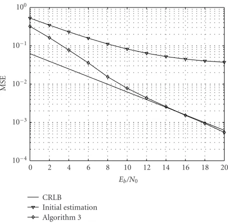
channel models to study the effect of the number of iterations needed to converge.Figure 11shows the BER performance of Algorithm 3 andFigure 12displays the corresponding MSE.
100
10−1
10−2
10−3
BER
0 2 4 6 8 10 12 14 16 18 20
Eb/N0
Perfect CIR Initial estimation Algorithm 3
Figure 11: BER versusEb/N0 in the 8-path channel model using
Algorithm 3.
100
10−1
10−2
10−3
10−4
MSE
0 2 4 6 8 10 12 14 16 18 20
Eb/N0
CRLB
Initial estimation Algorithm 3
Figure12: MSE versusEb/N0 in the 8-path channel model using
Algorithm 3.
Similar conclusions can be drawn about the performance of BER and MSE as with Algorithms 1 and 2.
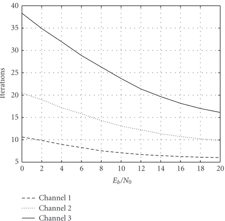
Figure 13shows the relationship between the number of iterations needed for convergence versus the channel delay spreadLfor differentEb/N0. From this figure, we observe that
the number of iterations decreases whenEb/N0increases; the
number of iterations increases when the channel delay spread increases under the sameEb/N0. Furthermore, we see that the
40 35 30 25 20 15 10 5
It
er
ations
0 2 4 6 8 10 12 14 16 18 20
Eb/N0
Channel 1 Channel 2 Channel 3
Figure 13: The number of iterations versusEb/N0 in the 8-path
channel model using Algorithm 3.
100
10−1
10−2
10−3
10−4
MSE
0 2 4 6 8 10 12 14 16 18 20
Eb/N0
Scheme 1 Scheme 2
Scheme 3 CRLB
Figure14: MSE versusEb/N0in the 8-path model using Algorithm
3. Three different schemes of the setβiare compared.
iterations approximately doubles. Therefore, this algorithm is more suitable for the case of small channel delay spread.
Figure 14shows the MSEs using different sets ofβiover
the 8-path channel. Scheme 1 corresponds to βi = 1/8.
Scheme 2 corresponds to βi = E{h2i} = e−i/C3. Scheme 3
corresponds toβiequal to the energy ofith path obtained in
each iteration. It changes from iteration to iteration. From this figure, we find that Scheme 1 has the best MSE perfor-mance and the other two schemes have larger MSE, especially in the large Eb/N0 region. Furthermore, Scheme 1 is
sim-pler than the other two since it only needs to knowL, while Scheme 2 has to know the average energy of each path of the
channel and Scheme 3 has additional computation in each iteration. Based on these preliminary simulations, it appears that Scheme 1 has the best performance without additional knowledge of the channel and additional computation.
5.4. Performance in different time-varying channels
Since the three algorithms show similar performance pat-terns, we choose Algorithm 2 to display the channel esti-mation performance in various time-varying channels with fdT = 0.01, 0.03, and 0.05, respectively. Some interesting
observations can be noted from Figures15 and16. As fdT
increases, that is, the channel varies faster, the performance of our algorithms degrades. However, the degradation is not so significant, especially when fdT ≤ 0.03. The
pi-lot pattern definitely affects the channel estimation and sys-tem performance [10]. However, our algorithms show sim-ilar performance with different number of pilot symbols in the frequency domain as long as Nf ≥ M/L. Most
per-formance degradation comes from the time-varying nature of the channel. For those fast time-varying channels (e.g., fdT = 0.05), reducing the pilot spacing along the time
do-main will improve the system performance as well as chan-nel estimation accuracy. But, for slowly and moderately time-varying channels (e.g., fdT=0.01 and 0.03), it does not help
much as our algorithms have already achieved near-optimal performance. Thus, our algorithms are able to achieve near-optimal performance by using very few pilot symbols both for slowly and fast time-varying channels.
5.5. Comparison with existing methods
In order to compare the performance with existing meth-ods, we choose the method with MMSE in the frequency domain [8] and linear interpolation (LI) in the time do-main [7] (MMSE + LI) as an example, since MMSE esti-mation in the frequency domain demonstrates a good and robust performance. The reason to use LI in the time do-main is to make the demodulation latency and necessary memory requirement as small as possible. For example, if Nt=8, the largest demodulation latency is 7 OFDM frames’
period and 9 OFDM frames’ data must be stored in the memory. ComparingFigure 17withFigure 15andFigure 18 withFigure 16, it is obvious that MMSE + LI performs much worse under the same channel model and pilot pattern, es-pecially in the high SNR region. Our algorithms are CRLB achievable, whereas MMSE + LI is not. Furthermore, there is an error floor for MSE in fast time-varying channels us-ing MMSE + LI. In order to remove it, more pilot symbols in the time domain must be inserted. This will reduce the system spectrum efficiency. Another advantage of our algo-rithms is that they do not have demodulation latency except the processing time because our algorithms are based on the received signals of the current OFDM frame. MMSE + LI or other pilot-symbols-assisted channel estimation methods have some extent of demodulation latency as long as they ap-ply some kinds of time-domain interpolation or filtering.
100
10−1
10−2
10−3
BER
0 2 4 6 8 10 12 14 16 18 20
Eb/N0
Perfect CIR
fdT=0.01, Nf =8, Nt=8
fdT=0.01, Nf =4, Nt=8
fdT=0.01, Nf =8, Nt=4
fdT=0.03, Nf =8, Nt=8
fdT=0.03, Nf=4, Nt=8
fdT=0.03, Nf=8, Nt=4
fdT=0.05, Nf=8, Nt=8
fdT=0.05, Nf=4, Nt=8
fdT=0.05, Nf=8, Nt=4 Figure15: BRE through time-varying channels with different fdT
of Algorithm 2.
100
10−1
10−2
10−3
10−4
MSE
0 2 4 6 8 10 12 14 16 18 20
Eb/N0
CRLB
fdT=0.01, Nf=8, Nt=8
fdT=0.01, Nf=4, Nt=8
fdT=0.01, Nf=8, Nt=4
fdT=0.03, Nf=8, Nt=8
fdT=0.03, Nf =4, Nt=8
fdT=0.03, Nf =8, Nt=4
fdT=0.05, Nf =8, Nt=8
fdT=0.05, Nf =4, Nt=8
fdT=0.05, Nf =8, Nt=4 Figure16: MSE of channel estimates through time-varying chan-nels with different fdTof Algorithm 2.
select Nt = 8, Nf = 8, and L = 8 as the
correspond-ing system parameters. MMSE + LI needsM/8 + 2 complex-variable multiplications per subcarrier. Algorithms 1, 2, and 3 need 17 + 2 log2M, 10 + log2M, and 26 + log2M complex-variable multiplications per subcarrier per iteration. Obvi-ously, the complexity of our algorithms is larger than the
100
10−1
10−2
10−3
BER
0 2 4 6 8 10 12 14 16 18 20
Eb/N0
Perfect CIR
fdT=0.01, Nf=8, Nt=8
fdT=0.01, Nf=4, Nt=8
fdT=0.01, Nf=8, Nt=4
fdT=0.03, Nf=8, Nt=8
fdT=0.03, Nf =4, Nt=8
fdT=0.03, Nf =8, Nt=4
fdT=0.05, Nf =8, Nt=8
fdT=0.05, Nf =4, Nt=8
fdT=0.05, Nf =8, Nt=4 Figure17: BER through time-varying channels with different fdT
of MMSE + LI.
100
10−1
10−2
10−3
10−4
MSE
0 2 4 6 8 10 12 14 16 18 20
Eb/N0
CRLB
fdT=0.01, Nf=8, Nt=8
fdT=0.01, Nf=4, Nt=8
fdT=0.01, Nf=8, Nt=4
fdT=0.03, Nf=8, Nt=8
fdT=0.03, Nf=4, Nt=8
fdT=0.03, Nf=8, Nt=4
fdT=0.05, Nf=8, Nt=8
fdT=0.05, Nf=4, Nt=8
fdT=0.05, Nf=8, Nt=4 Figure18: MSE of channel estimates through time-varying chan-nels with different fdTof MMSE + LI.
104
Figure19: Complexity comparison measured by complex-variable multiplications per subcarrier.
6. CONCLUSION
In this paper, we proposed three EM-based iterative algo-rithms to efficiently estimate the CIR and demodulate the transmitted signals in an OFDM system. By defining diff er-ent “complete” data sets for the EM algorithm, we are led to the three algorithms: (1) estimating the frequency response of the channel; (2) estimating the transmitted signals; and (3) estimating the CIR. Making use of a modest number of pilot symbols or the channel estimate of the previous OFDM frame to obtain the initial estimate, these algorithms can achieve near-optimal estimates after a few iterations. We also derived the CRLB and MCRB for the channel estimate for both constant and nonconstant modulus signals. Advantages and disadvantages of each algorithm have been discussed and illustrated by means of simulation. The simulations reveal that the first two (estimating the frequency response and demodulating the transmitted signals directly) converge at a rate independent of the multipath spread. Bypassing the channel estimate by demodulating the transmitted signals di-rectly (Algorithm 2) is the fastest converging procedure and, thus, has the smallest overall computational burden. Algo-rithm 2 has the least complexity among the three and is com-parable with MMSE + LI. However, the performance is much better than that of MMSE + LI, especially in the high SNR region. All three algorithms are able to work in a fast fad-ing environment. These algorithms can easily be extended to estimate multiple-input multiple-output (MIMO) channels in MIMO-OFDM systems. Our results indicate that the per-formance is acceptable only whenEb/N0is larger than 8 dB.
In the small SNR region, these algorithms need to be uti-lized with channel coding schemes to further improve per-formance.
Then differentiating the last expression with respect toH, and setting it to zero, we have
˜
C. DERIVATION OF ALGORITHM 2
Equation (27) can be rewritten as follows:
QXX(p)= logf(Y,h|X)fhY,X(p)dh, (C.1)
where the log-likelihood function can be expressed as fol-lows:
logf(Y,h|X)=logf(Y|h,X) + logf(h|X). (C.2)
The conditional pdf f(h|Y,X(p)) is used in (C.1) to take
of maximization in (28), theQfunction of (C.1) can be
re-where we use the assumption thathandX(p)are independent
of each other. Thus, (C.3) can be further reduced to
QXX(p)∝ logf(Y|h,X)fYh,X(p)f(h)dh,
(C.5)
since f(Y|X(p)) does not depend onX. Hence, it can be dis-carded in the last expression.
We now compute the above Q(X|X(p)) for a fading
whereσ2is the variance of both real and imaginary
compo-nents of complex-valued Gaussian white noise. The pdf f(h) is given by complex-valued CIR vectorh. By omitting the constant term and the scaling factor, (C.3) can be expressed as follows:
QXX(p)∝ − Y−XWLDh2f
estimated posterior mean and posterior covariance matrix at
thepth iteration and are given by
h(p)=Σ(p)WH
Maximizing (C.8) is equivalent to minimizing the dis-tance
This minimization can be further simplified as follows:
max
Since the distribution of random vectorY givenhand X(p)is Gaussian with meanh(p)and covariance matrixΣ(p), it is easy to compute
EhHF+FHhY,X(p)=h(p)H
F+FHh(p). (C.15)
Moreover, all entries of matrixGare given in terms of the signal energies, that is, |X(0)|2,. . .,|X(M−1)|2. Thus, we
can compute the third part of (C.12) as follows:
EhHGhY,X(p)=
andΣ(p)and can be obtained by the following equation:
Cm=
Equation (C.19) can be solved as follows:
where CD = diag(C,. . .,C)MD×MD andC = diag(C20,. . .,
D. DERIVATION OF ALGORITHM 3
Equation (43) can be rewritten as follows:
QZh(p)
whereK1andK2are some constants independent ofh, and
ˆ
whereβi=σi2/σ2are real-valued scalars satisfying
L−1
The above minimization problem can be separated into L simple minimization problems by just exchanging the order
of the two summations. TheseLminimization problems are
h(ip+1)=arg minh which can be solved by
h(ip+1)=
E. DERIVATION OF CRLB
In [25], the authors derive the CRLB by separating the com-plex vectorhinto real and imaginary parts. We will simplify the derivation by applying derivatives with respect to the complex vector itself. Recall the OFDM system model can be represented as in (26), where we use the same notation as in Section 3.3. We again assume for generality that the channel is static over the period ofDframes. We will derive a CRLB by using all the data from theDframes. The parameter vec-tor here is obviouslyθ =h. The CRLB gives a lower bound [28] for the variance of an unbiased estimate:
CRLBhi
=I−1(h)
ii, 0≤i≤L−1, (E.1)
whereI(h) is the Fisher information matrix
I(h)= −E ∂
Following (26), we have the conditional pdf ofYgivenh:
f(Y|h)= 1
where we assume the data matrixXis known. Therefore, the pdf is not conditioned onX. After differentiating the loga-rithm of (E.3) with respect toh, we obtain
Then the Fisher information matrix is obtained as follows:
I(h)=E ∂
CRLB for the overall CIR as follows:
ACKNOWLEDGMENT
This work has been supported, in part, by Grants from the New Jersey Center for Wireless Telecommunications (NJCWT), the National Science Foundation (NSF), Mit-subishi Electric Research Labs, Murray Hill, NJ, and Mi-crosoft Fellowship Program.
REFERENCES
[1] L. J. Cimini Jr., “Analysis and simulation of a digital mo-bile channel using orthogonal frequency division multiplex-ing,”IEEE Trans. Communications, vol. 33, no. 7, pp. 665–675, 1985.
[2] S. B. Weinstein and P. M. Ebert, “Data transmission by frequency-division multiplexing using the discrete Fourier transform,” IEEE Trans. Communications, vol. 19, no. 5, pp. 628–634, 1971.
[3] H. Sari, G. Karam, and I. Jeanclaude, “Transmission tech-niques for digital terrestrial TV broadcasting,”IEEE Commu-nications Magazine, vol. 33, no. 2, pp. 100–109, 1995. [4] Y. Li, L. J. Cimini Jr., and N. R. Sollenberger, “Robust
chan-nel estimation for OFDM systems with rapid dispersive fad-ing channels,”IEEE Trans. Communications, vol. 46, no. 7, pp. 902–915, 1998.
[5] J. K. Moon and S. I. Choi, “Performance of channel estimation methods for OFDM systems in a multipath fading channels,” IEEE Transactions on Consumer Electronics, vol. 46, no. 1, pp. 161–170, 2000.
[6] P. Hoeher, S. Kaiser, and P. Robertson, “Two-dimensional pilot-symbol-aided channel estimation by Wiener filtering,” inProc. IEEE Int. Conf. Acoustics, Speech, Signal Processing (ICASSP ’97), vol. 3, pp. 1845–1848, Munich, Germany, April 1997.
[7] F. Said and A. H. Aghvami, “Linear two dimensional pilot assisted channel estimation for OFDM systems,” inProc. 6th IEE Conference on Telecommunications, pp. 32–36, Edinburgh, UK, March–April 1998.
[8] J.-J. van de Beek, O. Edfors, M. Sandell, S. K. Wilson, and P. O. Borjesson, “On channel estimation in OFDM systems,” in Proc. 45th IEEE Vehicular Technology Conference (VTC ’95), vol. 2, pp. 815–819, Chicago, Ill, USA, July 1995.
[9] O. Edfors, M. Sandell, J.-J. van de Beek, S. K. Wilson, and P. O. Borjesson, “OFDM channel estimation by singular value de-composition,”IEEE Trans. Communications, vol. 46, no. 7, pp. 931–939, 1998.
[10] R. Nilsson, O. Edfors, M. Sandell, and P. O. Borjesson, “An analysis of two-dimensional pilot-symbol assisted modula-tion for OFDM,” inProc. IEEE International Conference on Personal Wireless Communications (ICPWC ’97), pp. 71–74, Mumbai, India, December 1997.
[11] B. Yang, K. B. Letaief, R. S. Cheng, and Z. Cao, “Channel esti-mation for OFDM transmission in multipath fading channels based on parametric channel modeling,” IEEE Trans. Com-munications, vol. 49, no. 3, pp. 467–479, 2001.
[12] R. W. Heath Jr. and G. B. Giannakis, “Exploiting input cy-clostationarity for blind channel identification in OFDM sys-tems,” IEEE Trans. Signal Processing, vol. 47, no. 3, pp. 848– 856, 1999.
[13] B. Muquet and M. de Courville, “Blind and semi-blind chan-nel identification methods using second order statistics for OFDM systems,” inProc. IEEE Int. Conf. Acoustics, Speech, Sig-nal Processing (ICASSP ’99), vol. 5, pp. 2745–2748, Phoenix, Ariz, USA, March 1999.
[14] X. Cai and A. N. Akansu, “A subspace method for blind chan-nel identification in OFDM systems,” inProc. IEEE Interna-tional Conference on Communications (ICC ’00), vol. 2, pp. 929–933, New Orleans, La, USA, June 2000.
[15] X. Zhuang, Z. Ding, and A. L. Swindlehurtst, “A statistical subspace method for blind channel identification in OFDM communications,” inProc. IEEE Int. Conf. Acoustics, Speech, Signal Processing (ICASSP ’00), vol. 5, pp. 2493–2496, Istan-bul, Turkey, June 2000.
[16] C. Li and S. Roy, “Subspace based blind channel estimation for OFDM by exploiting virtual carrier,” inProc. IEEE Global Telecommunications Conference (GLOBECOM ’01), vol. 1, pp. 295–299, San Antonio, Tex, USA, November 2001.
[17] P. Chen and H. Kobayashi, “Maximum likelihood channel estimation and signal detection for OFDM systems,” inProc. IEEE International Conference on Communications (ICC ’02), vol. 3, pp. 1640–1645, New York, NY, USA, April–May 2002. [18] S. Zhou and G. B. Giannakis, “Finite-alphabet based channel
estimation for OFDM and related multicarrier systems,”IEEE Trans. Communications, vol. 49, no. 8, pp. 1402–1414, 2001. [19] A. P. Dempster, N. M. Laird, and D. B. Rubin, “Maximum
likelihood from incomplete data via the EM algorithm,” Jour-nal of the Royal Statistical Society (B), vol. 39, no. 1, pp. 1–38, 1977.
[20] T. K. Moon, “The expectation-maximization algorithm,” IEEE Signal Processing Magazine, vol. 13, no. 6, pp. 47–60, 1996.
[21] H. Zamiri-Jafarian and S. Pasupathy, “EM-based recursive es-timation of channel parameters,” IEEE Trans. Communica-tions, vol. 47, no. 9, pp. 1297–1302, 1999.
[22] C. N. Georghiades and J. C. Han, “Sequence estimation in the presence of random parameters via the EM algorithm,”IEEE Trans. Communications, vol. 45, no. 3, pp. 300–308, 1997. [23] L. M. Zeger and H. Kobayashi, “A simplified EM algorithm
for detection of CPM signals in a fading multipath channel,” Wireless Networks, vol. 8, no. 6, pp. 649–658, 2002.
[24] M. Feder and E. Weinstein, “Parameter estimation of super-imposed signals using the EM algorithm,”IEEE Trans. Acous-tics, Speech, and Signal Processing, vol. 36, no. 4, pp. 477–489, 1988.
[25] M. Morelli and U. Mengali, “A comparison of pilot-aided channel estimation methods for OFDM systems,” IEEE Trans. Signal Processing, vol. 49, no. 12, pp. 3065–3073, 2001. [26] R. W. Miller and C. B. Chang, “A modified Cram´er-Rao bound and its applications (Corresp.),” IEEE Transactions on Information Theory, vol. 24, no. 3, pp. 398–400, 1978. [27] A. N. D’Andrea, U. Mengali, and R. Reggiannini, “The
mod-ified Cramer-Rao bound and its application to synchroniza-tion problems,”IEEE Trans. Communications, vol. 42, no. 234, pp. 1391–1399, 1994.
[28] S. M. Kay, Fundamentals of Statistical Signal Processing: Es-timation Theory, Prentice-Hall, Englewood Cliffs, NJ, USA, 1993.
Xiaoqiang Mareceived the B.E. and M.S. degrees in electrical engineering from Ts-inghua University, Beijing, China, in 1996 and 1999, respectively, and is now pursu-ing the Ph.D. degree in electrical engineer-ing from Princeton University. He was with Mitsubishi Lab, Murryhill, NJ, during the summer of 2000 and with Microsoft Re-search, Redmond, Wash, during the sum-mer of 2003. His research interests are in the
Hisashi Kobayashiis the Sherman Fairchild University Professor of Electrical Engineer-ing and Computer Science at Princeton University, NJ, since 1986, when he joined the Princeton faculty as the Dean of the School of Engineering and Applied Science (1986–1991). He worked for the IBM Re-search Center in Yorktown Heights for fif-teen years (1967–1982), and then served as the Founding Director of the IBM Tokyo
Research Laboratory (1982–1986). He was a radar designer at Toshiba, Japan (1963-1965). He received his Ph.D. from Prince-ton University in 1967, and his B.E. and M.E. degrees from the University of Tokyo in 1961 and 1963, respectively. His research experiences include radar systems, high speed data transmission, seismic signal processing, coding for high density digital recording, image compression algorithms, performance modeling and analy-sis of computers and communication systems. His current research activities include network security, OFDM and UWB communica-tion systems, and network performance modeling. He has been a Fellow (1977) and a Life Fellow (2003) of IEEE, and received the Humboldt Prize from Germany (1979). He was elected a Member of the Engineering Academy of Japan (1992) and a Fellow of IEICE, Japan (2004).
Stuart C. Schwartz received the B.S. and M.S. degrees from MIT in 1961 and the Ph.D. degree from the University of Michi-gan in 1966. At MIT, he was associ-ated with the Naval Supersonic Laboratory and the Instrumentation Laboratory (now the Draper Laboratories). During the year 1961–1962, he was at the Jet Propulsion Laboratory in Pasadena, California, work-ing on problems in orbit estimation and