R E S E A R C H
Open Access
Collaborative emitter tracking using
Rao-Blackwellized random exchange diffusion
particle filtering
Marcelo G S Bruno
1*†and Stiven S Dias
1,2†Abstract
We introduce in this paper the fully distributed, random exchange diffusion particle filter (ReDif-PF) to track a moving emitter using multiple received signal strength (RSS) sensors. We consider scenarios with both known and unknown sensor model parameters. In the unknown parameter case, a Rao-Blackwellized (RB) version of the random exchange diffusion particle filter, referred to as the RB ReDif-PF, is introduced. In a simulated scenario with a partially connected network, the proposed ReDif-PF outperformed a PF tracker that assimilates local neighboring measurements only and also outperformed a linearized random exchange distributed extended Kalman filter (ReDif-EKF). Furthermore, the novel ReDif-PF matched the tracking error performance of alternative suboptimal distributed PFs based respectively on iterative Markov chain move steps and selective average gossiping with an inter-node communication cost that is roughly two orders of magnitude lower than the corresponding cost for the Markov chain and selective gossip filters. Compared to a broadcast-based filter which exactly mimics the optimal centralized tracker or its equivalent (exact) consensus-based implementations, ReDif-PF showed a degradation in steady-state error performance. However, compared to the optimal consensus-based trackers, ReDif-PF is better suited for real-time applications since it does not require iterative inter-node communication between measurement arrivals.
Keywords: Distributed particle filters; RSS emitter tracking; Diffusion; Wireless sensor networks
1 Introduction
In several engineering applications, e.g., target tracking or fault detection, multiple agents [1] that are physically dispersed over remote nodes on a network cooperate to execute a global task, e.g., estimating a hidden signal or parameter, without relying on a global data fusion cen-ter. Each network node is normally equipped with one or more sensors that generate local measurements and can process those measurements independently of the rest of the network. At the same time, however, the net-work nodes are also able to communicate with each other in order to build in a collaborative fashion a joint esti-mate of the hidden signals or parameters of interest that depends both on local and remote measurements. Ide-ally, that joint estimate should be equal to or, at least
*Correspondence: [email protected] †Equal contributors
1Instituto Tecnológico de Aeronáutica, Praça Marechal Eduardo Gomes 50, São José dos Campos, Sao Paulo 12228-900, Brazil
Full list of author information is available at the end of the article
approximate the optimal global estimate that would be generated by a centralized processor with access to all network measurements.
Most of the previous literature in distributed signal processing on networks is based on linear estimation methods. Specifically, distributed versions of the Kalman filter were proposed e.g., in [2-4] to track unknown state vectors in linear, Gaussian state-space models. In situ-ations, however, where the state dynamic model or the sensor observation models are nonlinear, the posterior distribution of the states conditioned on the network mea-surements becomes non-Gaussian (even with Gaussian sensor noise) and, therefore, the linear minimum mean square error (LMMSE) estimate of the states provided, e.g., by an extended Kalman filter (EKF) may differ from the true minimum mean square error (MMSE) estimate given by the expected value of the state vector conditioned on the measurements. In this paper in particular, we focus specifically on an application where multiple pas-sive received-signal-strength (RSS) sensors jointly track
a moving emitter assuming, at each network node, non-linear observation models with possibly unknown static parameters.
1.1 Distributed particle filtering
In nonlinear scenarios, an alternative to approximate the true MMSE estimate is to use a sequential Monte Carlo method like particle filters [5,6]. Several distributed par-ticle filters have been proposed recently, see a compre-hensive review in [7], to handle nonlinear distributed estimation tasks. An important constraint in the design of a distributed estimation algorithm is, however, that most networks of practical interest are only partially connected, i.e., each node can only directly access neighboring nodes in its immediate vicinity according to the network topol-ogy. In particular, assuming conditional independence of the different sensor measurements given the state vec-tor, a distributed particle filter (PF) normally requires the computation of a product of likelihood functions that depend on local data only [8]. To compute that product over the network in a fully distributed fashion and with local neighborhood inter-node communication only, pre-vious references suggest using iterative average consensus [8], iterative Markov chain Monte Carlo move steps [9], or selective gossip algorithms [10]. Alternatively, we pro-posed in [11] to compute the likelihood product exactly in a finite number of iterations using either iterative min-imum consensus [12] or flooding techniques [13]. How-ever, both consensus or flooding-based solutions are very costly in terms of bandwidth requirements as they require multiple iterative inter-node communication between two consecutive sensor measurements. Previous works, e.g. [8,14,15], propose approximations aimed at reducing the communication cost, but, in all aforementioned schemes, processing and sensing at different time scales are still required.
1.2 Diffusion particle filtering
An alternative to circumvent the high communication cost of consensus algorithms is to use diffusion algorithms [16] which, contrary to the former, do not require multiple iterative inter-node communication between consecutive measurements. Diffusion algorithms are, however, sub-optimal in the sense that they do not simulate at each time step the behavior of the optimal global estimator, but rather, at best, approximate the optimal global solution asymptotically over time.
In the distributed linear estimation literature, most dif-fusion schemes are based on convex combinations of Kalman filters, see e.g., [3]. Kar et al. proposed in [2] a different approach based on random information dissemi-nation. In a previous conference paper [17], we introduced the random exchange diffusion particle filter (ReDif-PF),
which generalizes and extends the methodology in [2] to a PF framework by basically using random informa-tion disseminainforma-tion to build at each network node different Monte Carlo representations of the posterior distribution of the states conditioned on random sets of measurements coming from the entire network. Reference [17] assumed, however, that the parameters of the sensor observation model were perfectly known. In this paper, we extend the algorithm to a scenario with unknown parameters and derive in detail a Rao-Blackwellized [18] version of the ReDif-PF. In the specific application under consideration in the paper, the unknown parameters are the sensor vari-ances, but most of the methodology in the derivation of the RB ReDif-PF is general and could be easily adapted to other signal models and applications provided that, in a fully Bayesian framework, the dynamic posterior prob-ability distribution of the unknown parameters condi-tioned on the observations and on the simulated particles is a conjugate prior[19] for the likelihood function of the measurements.
An abbreviated description of the RB ReDif-PF may be found also in the short paper [20]. This paper consolidates and extends both [17] and [20] including detailed deriva-tions and additional simulation results and comparisons. We also detail approximate versions of the RB ReDif-PF where we use Gaussian mixture models (GMM) [21] and moment-matching techniques inspired by [22] to reduce communication requirements.
1.3 Paper outline
Appendices 1 and 2 show the proof of some key results in the paper, and Appendix 3 describes the ReDif-EKF algorithm used for comparison purposes in Section 5.
2 Problem setup
For simplicity of notation, we use lowercase letters in this paper to denote both random variables/vectors and real-valued samples of random variables/vectors with the proper interpretation implicit in context.
Without loss of generality, we assume that the emit-ter trajectory is described by the white noise acceleration model [24]
is the hidden state vector at time step nconsisting of the positions and velocities of the target’s centroid respectively in dimensionsx andy; F is the state transition matrix; and {un} is a sequence of independent, identically distributed (i.i.d.) zero-mean Gaussian vectors with covariance matrix Q. MatricesF andQ, parameterized by the sampling periodT and the acceleration noiseσaccel2 , are detailed in [11,24].
2.1 Observation model
LetN(m,σ2)denote the Gaussian probability distribution with meanmand varianceσ2and denote byIG(a,b)the inverse-gamma probability distribution with parametersa andb. The measurementszr,0:n = zr,0,. . .,zr,nin deci-bels relative to one milliwatt (dBm) at therth node of a network ofRRSS sensors are modeled as
zr,n=gr(xn)+
where xr represents the rth sensor position, ||.|| is the Euclidean norm,(P0,d0,ζr)are known model parameters (see [25] for details), andHis a 2×4 projection matrix such thatH(1, 1)=H(2, 3)=1 andH(i,j)=0 otherwise. We also denote byNrthe set of nodes in the neighborhood of noder. The real-valued constants{α,β}are the model’s hyper-parameters.
Note that in (2), we take a fully Bayesian approach and model the unknown sensor noise variances σr2, r ∈ R, as random variables that are mutually independent for s = r and identically distributed a priori with an inverse-gamma distribution.
2.2 Problem statement and goals Letz1:R,0:ndenote the set
zr,t
for all network nodesr= 1,. . .,Rand all time instantst = 0,. . .,n. Givenz1:R,0:n, we want to compute the MMSE estimate
ˆ conditional expectation ofxngivenz1:R,0:n.
In the sequel, we first describe in Section 3 a recursive, centralized PF algorithm that approximates the desired global MMSE in (4) at each time stepnin a scenario with unknownsensor variance scalesσr2. Next, we review in Section 3.1 two fully distributed algorithms that operate on a partially connected network and allow exact in-network computation of the state estimate in (4) without a global data fusion center and with inter-node com-munication limited to a node’s immediate neighborhood according to the network topology. The network connec-tivity is described by a graph G = (R,E) where R = {1,. . .,R}is the set of nodes and the graph has an edge (u,v)∈E,(u,v)∈R×Rif and only if nodesuandvcan communicate directly with each other. The particular net-work graph used in the simulation scenarios in this paper is described in detail in Section 5.
Finally, we introduce in Section 4 a novel diffusion-based algorithm, which is also fully distributed and relies on local inter-node communication only specified as before by the network graphGbut, rather than yielding an identical estimate (4) at each node, obtains at each noder a suboptimal estimate ferent at each noderand includes measurements coming from random locations in the entire network, as opposed to measurements coming only from noderand its neigh-borhood. Compared to the exact distributed implemen-tations of the optimal global estimate in Section 3.1, the diffusion solution in Section 4, although suboptimal, is designed to have a much lower inter-node communica-tion cost and, therefore, is better suited for real-time applications.
3 Centralized particle filter
wherex(nq)
,q∈Q{1,. . .,Q}, with the corresponding
importance weightsw(nq)
is a properly weightedMonte Carlo set [5,6] that represents the posterior probability density function (PDF)p(xn|z1:R,0:n)in the sense that the sum on the right-hand side of (6) converges, according to some statistical criterion, to the expectation on the left-hand side when Q → ∞. The random samples
x(nq)
, also called particles, are sequentially generated according to a proposal probability distribution specified by a so-called importance PDF π(xn|x0:n(q)−1,z1:R,0:n). If the blind importance function [5]
π(xn|x(0:nq)−1,z1:R,0:n)=p(xn|x(nq−)1)
is used, then it turns out that the proper importance weights must be updated according to the recursion [6]
w(nq)∝w(nq−)1p(z1:R,n|x(0:nq),z1:R,0:n−1) (7)
where∝denotes ‘proportional to,’z1:R,nis an alternative notation for the setzr,n,r ∈ R, and the proportional-ity constant on the right-hand side of (7) is chosen such that Qq=1w(nq) = 1. From the mutual independence assumptions in the model in Section 2, it follows that
p(z1:R,0:n|x0:n,σ1:R2 )=
From (8) and (9), it can be shown then that (see the proof in [11])
Substituting now (10) into (7), the centralized weight update rule reduces to
3.1 Equivalent distributed implementation of the centralized particle filter
Note that each factor λ(r,nq)(x(nq)) in the product on the right-hand side of (11) depends only on local observa-tions. In a fully connected network, assuming that all nodes r ∈ Rstart out at instant n−1 with the same
particles x(nq−)1
, they can all synchronously draw [26]
new particlesx(nq)
according top(xn|x(nq−)1), locally
com-pute their own local likelihood functions λ(r,nq)(x(nq)), and then broadcast them to the entire network until all nodes have all the remote likelihood functions and can compute the product on the right-hand side of (11). Synchronous multinomial resampling according to the global weights followed by regularization may follow (see [11]) to miti-gate particle degeneracy and impoverishment [5,6]. The algorithm described in this paragraph is referred to as the decentralized particle filter (DcPF) in [11] and [27].
As mentioned, however, in Section 1, real-world net-works are only partially connected and fully distributed computations of the product in (11) are needed. One possibility is to approximate the product using iterative average consensus [28] as proposed, e.g., in [8] and [29]. Alternatively, we introduced in [11] a fully distributed computation of the global weights in (11) using either iterative minimum consensus [12] or flooding [13]. Both algorithms assume only local communication between nodes in immediate neighborhoods and, to achieve an exact computation of the global weights, require only a finite number of iterative message exchanges between nodes in the time interval between two consecutive sensor measurements.
LetDdenote the diameter of the network graph, i.e., the maximum number of hops between any two nodes and, as before, denote byRthe number of nodes in the net-work. By runningR×Dconsecutive minimum consensus iterations [12] for each particleq, it is possible (see details in [11]) to build an identical ordered list of likelihood functions λ(r,nq)(x(nq))
, r ∈ R, at all nodes. Each node can then locally compute the product of the likelihoods as in (10) and obtain identical, optimal global impor-tance weightsw(nq)
. We refer to that (communication-intensive) minimum-consensus-based distributed track-ing algorithm as CbPFa.
is not included in noder’s list yet, it is inserted with a flag in its list. This procedure is guaranteed to converge in a finite number of iterations as soon as each node hasR distinct values in its ordered list of likelihoods. We refer to the flooding-based iterative tracker in this paper as the CbPFb algorithm.
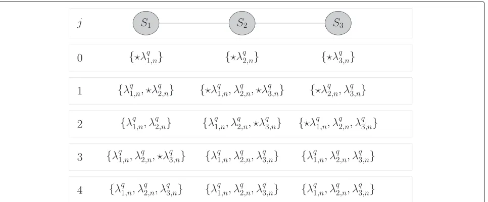
Figure 1 illustrates how the proposed flooding protocol iteratively creates at each noderan ordered list compris-ing all likelihoods across the network in a toy example with three nodes where node 1 is connected to node 2, node 2 is connected to nodes 1 and 3, and node 3 is connected to node 2 only. A star symbol is employed to indicate which likelihoods are flagged in the ordered list maintained by each noderat a given iterationj.
Although optimal in the sense of reproducing the cen-tralized solution, the minimum consensus and flood-ing algorithms in [11] are still communication-intensive due to the requirement of iterative inter-node commu-nication between sensor measurement arrivals. In the next sections, we describe an alternative fully distributed diffusion-based solution that drops this requirement and is the main topic of this paper.
4 Random exchange diffusion particle filter In this section, we derive an alternative distributed PF based on random information dissemination that extends the methodology in [2] to a Monte Carlo framework. We also present a Rao-Blackwellized version of the pro-posed distributed PF in a scenario with unknown sensor parameters.
Let Zs,0:n−1 denote the set of all network measure-ments assimilated by nodesup to instantn−1. Next, let
x(s,0:nq) −1
with associated weights w(s,nq)−1,q∈Q, be a properly weighted set that represents the posterior PDF
p(x0:n−1|Zs,0:n−1)at nodes. Assume now that at instant n−1, nodessends its particles and weights to a neigh-boring noderthat can assimilate at instantnthe measure-mentsZr,n =
zi,n
,i ∈ {r} ∪Nr. At instantn, the new particle set at noder,x(r,0:nq) =(xs,0:n(q) −1,x(r,nq))with updated weightsw(r,nq)such that
x(r,nq)∼p(xn|x(s,nq)−1) (12)
w(r,nq)∝w(s,nq)−1p(Zr,n|x(r,0:nq) ,Zs,0:n−1) (13)
is now a properly weighted set to represent the updated posterior p(x0:n|Zr,n,Zs,0:n−1), where {Zr,n, Zs,0:n−1} is redefined asZr,0:n. Resampling from the particle weights followed by regularization may be added to combat parti-cle degeneracy and restore partiparti-cle diversity, i.e., forq∈Q (see also [11]):
• Drawl(q)from{1, 2,. . .,Q}with
Pr({l(q)=l})=w(l)
r,n, wherePr(A)denotes the probability of an eventA.
• Makex¯(r,nq)=x(l (q))
r,n +hDnx∗, wherex∗∼N(0,I), DnDTn is equal to the empirical covariance of the weighted particles(x(r,nq),w(r,nq))
, andh>0is an empirically adjusted parameter.
• Reset the particle weightsw(r,nq)to Q1 and make x(r,nq)= ¯x(r,nq).
Random exchange protocol In order to build, at each instantnand at each noder, different Monte Carlo rep-resentations of the posterior distribution conditioned on different sets of observationsZr,0:ncoming from random
locations in the entire network, it suffices to implement a protocol where each noder, starting from instant zero, exchanges its particles and weights with a randomly cho-sen neighboring nodes, propagates the received particles using the blind importance function as in (12), and then updates their weights as in (13).
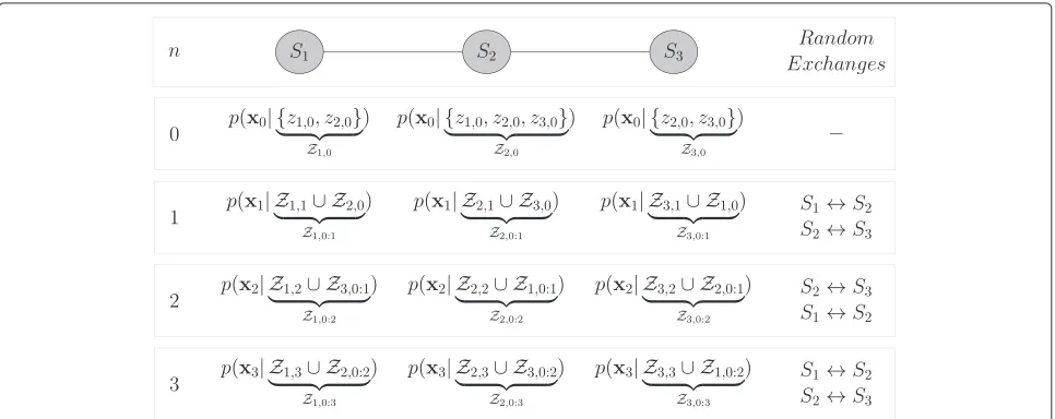
Figure 2 illustrates the evolution of the marginal poste-rior at each node - in a linear network containing three nodes running the random exchange protocol - over four time instants. Initially, each noder ∈ {1, 2, 3}has a pos-terior at instant zero conditioned on the measurements Zr,0= {zi,0},i∈ {r} ∪Nr, in its vicinity only. At each time instantn∈ {1, 2, 3}, network nodes perform the sequence of random exchanges as indicated in the rightmost col-umn of Figure 2 and, then, update the received pos-terior by assimilating measurements in their respective neighborhoods.
Note that in the linear network topology shown in Figure 2, node 2 always performs two random exchanges at each time instantn. Generally speaking, however, at a given instantn, a noderexchanges its parameters at least one time with a randomly chosen neighborsand, in the worst case, performsd(r)random exchanges between two measurement arrivals with nodes in its vicinity, whered(r) is the degree of noder, i.e., the number of neighbor nodes. Unlike randomized gossip algorithms [30], this proce-dure diffuses information by randomly propagating pos-terior statistics across the network. More specifically, as the initial posterior statistics provided by a given node r0 at time 0 follows a path P {r0,r1,. . .,rn} along the network, it assimilates the available measurements Zr,n in the neighborhood of each visited node r ∈ P. Since, as illustrated in Figure 2, the initial posteriors at each node follow different paths, the posterior available
at node rn at time n will be different from those in the remaining nodes. Thus, network nodes will pro-vide different estimates conditioned on distinct sets of measurements.
4.1 ReDif-PF with known sensor variances
If the parameters of the sensor observation model at each noderare deterministic and perfectly known, then
p(Zr,n|xr,0:n(q) ,Zs,0:n−1)=
i∈{r}∪Nr
p(zi,n|x(r,nq)). (14)
At instantn, then, upon receiving(w(s,nq)−1,xs,n(q)−1),q∈Q, from nodes, the particle filter at nodersamples as before
xr,n(q)∼p(xn|xs,n(q)−1) q=1,. . .,Q
and updates its weights as
w(r,nq)∝w(s,nq)−1
i∈{r}∪Nr
p(zi,n|xr,n(q)) q=1,. . .,Q
(15)
wherezi|x(r,nq)∼N(gi(x(r,nq)),σi2).
Inter-node transmission requirements From the previ-ous discussion, it follows that in the scenario with known variances at each instant n, it suffices for each node s to transmit to the chosen neighbor r the set of par-ticles {x(s,nq)−1} (4Q real numbers for a four-dimensional state space) and the respective set of importance weights {w(s,nq)−1}(Qreal numbers). In addition, nodesalso sends its scalar observation zs,n and the known observation model parameters( ζs,xs,σs2)(see (3)) to all nodesiin the neighborhood ofs.
4.2 Rao-Blackwellized ReDif-PF with unknown sensor variances
LetIG(σ2|α,β)denote the PDF of a continuous random variableσ2with an inverse-gamma distribution specified by the parametersαandβ, i.e. [19],
and zero otherwise. In (16), (.) denotes the gamma function Gaussian random vector taking values in L and with meanmand positive definite covariance matrix, i.e.,
N(x|m,)= 1
where||denotes the determinant of the matrix and the superscript T denotes the transpose of a vector.
In the scenario with unknownsensor variances, it can be shown (see Appendix 2) that if at instantn−1,
p(σ1:R2 |xs,0:n(q) −1,Zs,0:n−1)= on the right-hand side of (18) is computed by solving the integral
where(·), as before, denotes the gamma function
αr,i,n=αs,i,n−1+ instantn, the updated parameter posterior PDF
p(σ1:R2 |x(r,0:nq) ,Zr,0:n)=
ticle degeneracy, the posterior parameters{βs,i,n(q)−1}must be also resampled according to new weightsw(r,nq)updated as in (13) and a new set a different suboptimal strategy described in Section 4.3, which also allows a significant reduction in inter-node communication cost.
Inter-node transmission requirements In the un-known variance scenario, based on the previous discus-sion, at each instantn , a node s has to transmit to its (randomly chosen) neighboring node r its particle set
nodesalso sends its scalar observationzs,nand the obser-vation model parameters ( ζs,xs) to all nodes i in the neighborhood ofs.
4.3 Approximate RB ReDif-PF
Although the exact ReDif-PF algorithms in Sections 4.1 and 4.2 converge asymptotically to the state estimate in (5) as the number of particles Q goes to infinity, their inter-node communication cost is still relatively high. To reduce the communication burden, we propose two sub-optimalapproximations which are described in detail in the sequel.
param-eter scenarios, Q particles and respective weights per node at each time step, we follow the lead in [21] and build a GMM representation of the marginal posterior p(xn−1|Zs,0:n−1)of the form
p(xn−1|Zs,0:n−1)≈ k∈K
ηs,n(k)−1N(xn−1|μs,n(k)−1,(s,nk)−1)
(23)
whereK = {1,. . .,K}and the parametersηs,n(k)−1,μ(s,nk)−1, and (s,nk)−1 are obtained from the weighted particle set
xs,n(q)−1,ws,n(q)−1,q∈Q, at nodesusing the Expectation-Maximization (EM) [31] algorithm. Nodesnow transmits to node r only the parameters that specify the GMM model, i.e., 15Kreal numbers for a four-dimensional state vector, as opposed to 5Q real numbers, where typically Q >> K (in the simulations in Section 5 for exam-ple, K is either 1 or 2, whereas Qis 500). Node rthen locally resamplesQnew particlesx(s,nq)−1according to the received GMM PDF and resets its importance weights w(s,nq)−1to 1/Q. Since resampling from the GMM approxi-mation is used, we omit the regularization step mentioned in Section 4.
Approximation of the posterior distribution of the sensor variances In the particular situation where the sensor variances are unknown, in theory we should also locally resample the previous particle trajectoriesx(s,0:nq) −2 jointly withx(s,nq)−1from some parametric approximation top(x0:n−1|Zs,0:n−1)and then recompute retroactively the posterior PDF’sp(σi2|x(s,0:nq) −1,Zs,0:n−1), i = 1,. . .,Rfor the resampled particle paths. To eliminate that curse of dimensionality, it is desirable to introduce a parametric approximation top(σi2|xs,0:n(q) −1,Zs,0:n−1) that eliminates the dependence of that function on the particle labelqand the simulated sequencex(s,0:nq) −1.
Specifically, we follow the lead in [11,22,32], and, for each i ∈ R, approximate the marginal posteri-ors p(σi2|x(0:nq)−1,Zs,0:n−1) for all particle labels q and all possible sequences x(0:nq)−1 by a new inverse gamma PDF with parameters α˜s,i,n−1 and β˜s,i,n−1, independent of q and chosen such that the approximated PDF IG(σi2| ˜αs,i,n−1,β˜s,i,n−1) matches the first and second moments of
p(σi2|Zs,0:n−1)= p(σi2|x0:n−1,Zs,0:n−1)
× p(x0:n−1|Zs,0:n−1)
dx0:n−1 (24)
where the term on the left-hand side of (24) is the average (or expected value) ofp(σi2|x0:n−1,Zs,0:n−1)over all possi-ble realizations ofx0:n−1conditioned on the observations
Zs,0:n−1. Assuming now that{(w(s,nq)−1,x (q)
s,0:n−1)},q ∈ Q, is a properly weight set available at nodesat instantn−1 to representp(x0:n−1|Zs,0:n−1), we make the Monte Carlo approximation
p(σi2|Zs,0:n−1)≈ Q
q=1
ws,n(q)−1p(σi2|xs,0:n(q) −1,Zs,0:n−1).
(25)
On the other hand, from the assumption that p(σ1:R2 |
x(s,0:nq) −1,Zs,0:n−1)is a separable function factored as in (17), it follows that
p(σi2|xs,0:n(q) −1,Zs,0:n−1)=IG(σi2|αs,i,n−1,βs,i,n(q)−1)
and, therefore,
p(σi2|Zs,0:n−1)≈
Q
q=1
w(s,nq)−1IG(σi2|αs,i,n−1,βs,i,n(q)−1).
(26)
In the sequel, recall that if σ2 ∼ IG(α,β), then the respective mean and variance ofσ2are given by [19]
Eσ2 = β
α−1, α >1 (27)
Varσ2 = β
2
(α−1)2(α−2), α >2. (28)
Therefore, the parametersα˜s,i,n−1andβ˜s,i,n−1such that IG(σi2| ˜αs,i,n−1,β˜s,i,n−1) matches the mean and variance associated with the PDF on the right-hand side of (26) are found, following the procedure in [11,22,32] by making
˜
αs,i,n−1=2+E2s,n−1
σi2/VARs,n−1
σi2 (29)
˜
βs,i,n−1=(α˜s,i,n−1−1)Es,n−1
σi2, (30)
where
Es,n−1
σi2=
Q q=1w
(q) s,n−1β
(q) s,i,n−1
αs,i,n−1−1
(31)
VARs,n−1
σi2=
Q q=1w
(q) s,n−1(β
(q) s,i,n−1)2
(αs,i,n−1−1)(αs,i,n−1−2)
Replacing nowp(σi2|xs,0:n(q) −1,Zs,0:n−1)in (19) with
˜
p(σi2|Zs,0:n−1)=IG(σi2| ˜αs,i,n−1, β˜s,i,n−1)
for allq∈ {1,. . .,Q}andall possible sequencesx(s,0:nq) −1, we get, at noderat instantn, new factorsλ˜i,n(.)such that
˜
λi,n(x(q)r,n)= ∞
0
p(zi,n|x(q)r,n,σi2)p˜(σi2|Zs,0:n−1)dσi2
=
∞
0
N(zi,n|gi(x(q)r,n),σi2)IG(σi2| ˜αs,i,n−1,β˜s,i,n−1)dσi2
∝
˜
βs,i,n−1 α˜s,i,n−1
(α˜s,i,n−1)
(αr,i,n)
βr(q),i,nαr,i,n
,
(32)
where
αr,i,n= ˜αs,i,n−1+ 1
2 (33)
βr,i,n(q) = ˜βs,i,n−1+ 1 2
zi,n−gi(x(r,nq))
2
, (34)
for allq∈Qand alli∈ {r} ∪Nr. Otherwise, ifi∈ {r} ∪Nr
αr,i,n= ˜αs,i,n−1 (35)
βr,i,n(q) = ˜βs,i,n−1, (36)
again for all q ∈ Q. The modified importance weight update rule at noderat instantnnow becomes
w(r,nq)∝w(s,nq)−1
i∈{r}∪Nr
˜
λi,n(x(r,nq)) q∈ {1,. . .,Q}.
(37)
Inter-node communication cost By combining the GMM approximation and the moment-matching approx-imation described before, node s now transmits to its (randomly chosen) neighbor r only the GMM model parameters (15K real numbers as previously explained) plus 2R hyper-parameters (α˜s,i,n−1,β˜s,i,n−1), i ∈ R, as opposed toR×(Q+1)hyper-parameters as before in the exact RB ReDif-PF algorithm.
Summary of the approximate RB-ReDif-PF Algorithm 1 summarizes the approximate RB ReDif-PF tracker at node rat instant n. In Algorithm 1, the symbol r,n denotes the set η(r,nk), μr,n(k), (r,nk)
, α˜r,i,nβ˜r,i,n
for i ∈ R
andk∈K.
Algorithm 1 Approximate Rao-Blackwellized random exchange diffusion particle filter
1: procedureREDIF-PF(zr,n,s,n−1) 2: Sendzr,nto neighborsi∈Nr
3: Block until receive allzi,nfrom nodesi∈Nr 4: Extractη(s,nk)−1,μ(s,nk)−1,(s,nk)−1froms,n−1,k ∈ K
and resample x(s,nq)−1, for all q ∈ Q from the GMM approximation defined by those parameters.
5: Extract(α˜s,i,n−1,β˜s,i,n−1),i∈R, froms,n−1
6: forq←1toQdo
7: Samplex¯(r,nq)∼p(xn|x(s,nq)−1)
8: Computeαr,i,n andβr,i,n(q), for alli ∈ Rusing (33) to (36).
9: Compute w¯(r,nq) ∝ i∈{r}∪Nrλ˜i,n(x¯ (q) r,n) where
˜
λi,n(x¯(r,nq))is given by (32). 10: end for
11: Normalizew¯(r,nq)such thatqw¯ (q) r,n=1. 12: Makexˆr,n|n=Qq=1w¯
(q) r,nx¯(r,nq)
13: Computeα˜r,i,n andβ˜r,i,n from the weighted par-ticle set{(w¯(r,nq),x¯(r,nq))} using (29) and (30) for all i ∈ R.
14: Compute the parametersη(r,nk),μr,n(k), and(r,nk)of the GMM approximation top(xn | Zr,0:n)using the EM algorithm.
15: Exchanger,nwiths,nfrom a randomly chosen neighborsusing the random exchange protocol, see [17].
returnxˆr,n|n,s,n. 16: end procedure
4.4 Differences between ReDif-PF and the Markov chain distributed particle filter
An alternative and different approach to distributed par-ticle filtering is the MCDPF algorithm introduced in [9]. MCDPF, like other previous work in the distributed PF literature, assumes conditional independence of the sen-sor observations given the target state and, therefore, should be compared to the proposed ReDif-PF algorithm in this paper in the known sensor parameters scenario of Section 4.1 as opposed to the more general Rao-Blackwellized version of ReDif-PF proposed for unknown sensor parameters in Section 4.2.
chain specified byAbeing equal tor, r = 1,. . .,R, and J is total number of Markov chain move steps between consecutive sensor measurements, which is set by the user. Since the number of visits to the noderdivided byJ con-verges toφ (r) [9] asJ → ∞, it follows that ifJ is large enough so that particlex
nnot only visits all network nodes but also visits each node multiple times, then the aggre-gate update factor for its corresponding weight at the end of the random walk will approach
R
r=1
p(zr,n|xn), (38)
which, under the assumption of conditional indepen-dence of the sensor measurements given the target state, is the exact update factor for the optimal global weight associated with particle xn. For a finite and especially low number of move steps, MCDPF is no longer opti-mal, meaning that the choice of the parameterJ involves a tradeoff between inter-node communication cost and state estimation error.
Contrary to MCDPF, the proposed ReDif-PF does not attempt to compute the exact optimal global posterior PDFp(x0:n|z1:R,0:n)at all nodesr=1,. . .,Rat each instant n. Instead, as explained in previous sections, ReDif-PF builds at each noderand at each instantna Monte Carlo representation of the posteriorp(x0:n|Zr,0:n), whereZr,0:n is a random subset of z1:R,0:n that changes from node to node. Such Monte Carlo representation is built in a way that between instantsnandn+1, each node makes only one requestto exchange particles/weights (or equiv-alent parametric approximations of posterior distribu-tions) with a randomly chosen neighbor, thus eliminating the need for multiple iterative inter-node communication between consecutive sensor measurements and resulting in a communication cost that is much lower than that of the MCDPF algorithm for a similar mean square state estimation error (see the numerical simulation results in Section 5.2).
Finally, we also note that compared to the non-iterative ReDif-PF, MCDPF is also computationally more intensive since each node r has to compute the local likelihoods p(zr,n|xn(q)) for all its particles x(nq) multiple (namely J) times between instantsnandn+1. We also illustrate that point in the numerical simulations of Section 5.2.
5 Simulation results
We assessed the performance of the proposed algorithms using 100 Monte Carlo runs with simulated data in three distinct scenarios assuming both unknown and known sensor variances. In all scenarios, we usedR = 25 RSS sensors with parametersP0= 1 dBm,d0 = 1 m, ζr =3,
∀r ∈ R, and σr2 independently sampled at each node according to anIGdistribution with mean 16. The nodes
were deployed on a jittered grid within a square of size 100 m×100 m. In the fully distributed algorithms, each node communicates with other nodes within a range of 40 m. All particle filters usedQ=500 particles.
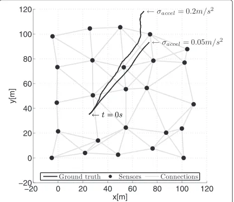
Figure 3 shows the sensor positions and two distinct realizations of the emitter trajectory generated forT = 1 s andx0 =
25 m 0.5 m/s 35 m 0.5 m/sT considering respectively σaccel = 0.05 m/s2 and σaccel = 0.2 m/s2. It also depicts the available network connections. The diameter of the sensor network isD = 5 hops and the minimum number of neighbors for any possible node is 3.
5.1 Scenario I: ReDif-PF vs. CbPF
In the first scenario, we assumed unknown sensor variances and evaluated the performance of the Rao-Blackwellized ReDif-PF and two consensus-based PF trackers using respectively iterative minimum consen-sus (CbPFa) and flooding (CbPFb) (see also [11]). The aforementioned algorithms were compared to the equiva-lent broadcast implementation of the optimal centralized PF tracker, referred to as DcPF in [11] and [27] and in Section 3.1 of this paper. We also assumed Gaussian priors with meanx0 y0
T
and covariance matrix diag(202, 202) for the emitter’s position in Cartesian coordinates and
mean
˙
x20+ ˙y20 arctan(y˙0/x˙0)
T
and covariance matrix
diag(0.32, (5π/180)2) for the emitter’s velocity in polar coordinates, where x0 = 25 m, y0 = 35 m, and x˙0 =
˙
y0 = 0.5 m/s. In the initialization step, the realiza-tions of the initial emitter velocity are sampled from the
Figure 3Evaluated scenario.Simulated scenario withR=25 RSS sensors deployed on a jittered grid within a square of size
aforementioned Gaussian prior and, then, converted from polar to Cartesian coordinates.
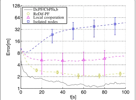
Figure 4 shows the evolution of the root mean square (RMS) error norm - averaged over all network nodes and Monte Carlo runs - of the emitter position estimates for the RB ReDif-PF and the CbPFa and CbPFb algo-rithms superimposed to the benchmark RMS error curve for the optimal DcPF algorithm. Furthermore, we also show in Figure 4 the average RMS error norm for the non-cooperative (isolated node) trackers and for a local cooperation scheme. In the former, each node runs a regularized PF tracker (see [11]) which assimilates local measurements only, while in the latter, a node r incor-porates all measurementsZr,nin its vicinity in the same way as in the ReDif-PF tracker, but it does not exchange its updated posterior with its neighbors. The bars shown in Figure 4 represent the standard deviation of the error norm across all nodes in the network. There are no bars for the DcPF and CbPF algorithms since they provide the same state estimate at all nodes. The RMS error norm at time step 0 for all algorithms was calculated after the mea-surements z1:R,0 were assimilated. We implemented the RB ReDif-PF in this scenario with the parametric approx-imations in Section 4.3 using only one Gaussian mode to representp(xn−1|Zs,0:n−1).
As expected, CbPFa and CbPFb match the performance of the DcPF tracker since both algorithms reproduce the optimal centralized PF tracker exactly, albeit with different communication and computational costs. On the other hand, as shown in Figure 4, the RB ReDif-PF tracker has a performance degradation compared to DcPF. This result is again theoretically expected since, in the RB ReDif-PF algorithm, the posterior at each node assimilates just a
0 20 40 60 80 100
1 2 4 8 16 32 64 128
Error[m]
t[s] DcPF/CbPFa,b ReDif-PF Local cooperation Isolated nodes
Figure 4Evolution of the estimated position RMS error norm. Performance comparison between the ReDif-PF and the
consensus-based algorithms assuming a Gaussian prior distribution around the initial emitter state in the first scenario withunknown sensor noise variances.
subset of the available measurementsz1:R,n in the whole network at each time step n. However, ReDif-PF offers an improvement in error performance compared to the local cooperation scheme by better diffusing the infor-mation across the network. We also note from Figure 4 that the standard deviation of the state estimate across the different network nodes is much lower in the ReDif-PF algorithm than in the local cooperation scheme. Note also that, as shown in Figure 4, isolated nodes were not able to properly track the emitter in the evaluated scenario.
Finally, Figure 5 shows the performance comparison between the ReDif-PF and consensus-based algorithms forσaccel∈ {0.05, 0.1, 0.2}.
As expected, as σaccel increases, there is a deterio-ration in the RMS error performance. However, the ratio between the RMS error performance of the sub-optimal ReDif-PF tracker and the benchmark sub-optimal DcPF/CbPFb algorithms remains approximately constant (close to a factor of two) along the simulation period for all three different values ofσaccelemployed.
Communication and computation cost Considering a four-byte and a one-byte network representation respec-tively for real and Boolean values, the total amount of bytes transmitted and received by all nodes over the net-work was recorded while running each tracker in Figure 4. Table 1 summarizes the communication cost for each algorithm in the first scenario (unknown sensor variances) in terms of average transmission (TX) and average recep-tion (RX) rates per node and also quantifies the processing cost for each algorithm in terms of average duty cycle per node, measured in a Intel Core i5 machine with 4GB RAM. The duty cycle of a given node is defined as the
0 20 40 60 80 100
1 2 4 8 16 32 64
Error[m]
t[s]
Table 1 Average communication and processing cost per node in the first scenario
RX rate TX rate Duty cycle (%)
DcPF 46.9 KB/s 2.0 KB/s 1.8
CbPFa 1.2 MB/s 244.1 KB/s 21.4
CbPFb 232.0 KB/s 48.7 KB/s 22.6
RB ReDif-PF 531.5 B/s 515.7 B/s 7.7
Local cooperation 4 B/s 19.8 B/s 9.3
Isolated nodes - - 2.0
ratio between the total node processing time and the sim-ulation period 100 s. Finally, values in Table 1 are averaged over all Monte Carlo simulations.
As shown in Table 1, the RB ReDif-PF tracker with the parametric approximations in Section 4.3 using only one Gaussian mode has a communication cost based on TX rate that is approximately one order of magnitude lower than the flooding-based CbPFb’s communication requirements. Compared to the iterative minimum con-sensus solution (CbPFa), the average communication cost is reduced by two orders of magnitude.
5.2 Scenario II: ReDif-PF vs. ReDif-EKF
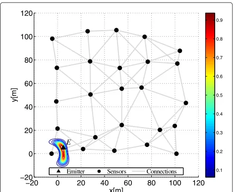
In the second scenario, the sensor variances are per-fectly known and the ReDif-PF tracker is compared both to the optimal centralized PF and to a linearized ran-dom exchange extended Kalman filter (ReDif-EKF), which is summarized in Appendix 3. In the simulations, we assumed a non-informative prior for the sensor’s ini-tial position that is uniform in the entire surveillance space. The actual initial position of the emitter was, how-ever, sampled from a Gaussian distribution centered at (5 m, 5 m)with standard deviation of 3 m in both dimen-sions. Figure 6 shows a normalized contour map for the posterior PDFp(x0,y0|z1:R,0)at instant 0 as a function of x0andy0assuming the aforementioned non-informative prior. As seen from Figure 6, the initial posterior distribu-tion of the target’s posidistribu-tion is non-Gaussian.
Figure 7 shows the evolution of the RMS error norm assuming known sensor variances respectively for the ReDif-PF algorithm in Section 4.1 with a two-Gaussian GMM parametric approximation and the ReDif-EKF algo-rithm in Appendix 3. We also show the RMS curve for the optimal centralized PF tracker as a benchmark. The plots in Figure 7 show that, especially in the initial time steps, when the posterior distribution of the states is strongly non-Gaussian as suggested by Figure 6, the fully distributed ReDif-PF outperforms its linearized counter-part, the ReDif-EKF. As the emitter moves away from the near field of the initial dominant sensor, the performance of the ReDif-EKF slowly improves and approaches that of the ReDif-PF, albeit still with a slight degradation towards the end of the simulation.
−20 0 20 40 60 80 100 120 −20
0 20 40 60 80 100 120
x[m]
y[m]
E
0.1 0.2 0.3 0.4 0.5 0.6 0.7 0.8 0.9
Emitter Sensors Connections
Figure 6Normalized PDF contour map at instant0.EmitterEnear sensor is in the bottom left corner.
Communication and Computation Cost Table 2 sum-marizes the communication and processing cost per node for each algorithm in the second scenario.
As expected, the DcPF algorithm assuming known sen-sor variances has the same communication requirements as in the scenario with unknown variances since DcPF locally computes the likelihood functions and then broad-casts them to the entire network. However, as shown in Table 2, DcPF has a slightly lower processing cost when the sensor variances are known. The ReDif-PF tracker on the other hand outperformed the ReDif-EKF tracker in terms of the position RMS error at the expense of a greater communication and computational cost. However, as indicated in Table 2, the communication requirements
0 20 40 60 80 100
1 2 4 8 16 32 64
Error[m]
t[s]
DcPF/CbPFb ReDif-PF ReDif-EKF
Table 2 Average communication and processing cost per node in the second scenario
RX rate TX rate Duty cycle (%)
DcPF 46.9 KB/s 2.0 KB/s 0.8
ReDif-PF 643.4 B/s 627.6 B/s 15.1
ReDif-EKF 131.8 B/s 116.0 B/s 0.08
of the ReDif-PF and ReDif-EKF trackers still have the same order of magnitude.
5.3 Scenario III: ReDif-PF vs. MCDPF/selective gossip In the third scenario, the ReDif-PF tracker is compared to two iterative algorithms from the literature - the MCDPF and the selective gossip from [9] and [23], respectively -assuming perfectly known sensor variances as in the second scenario and the same Gaussian priors for the emitter’s initial position and velocity used in the first scenario.
Figure 8 shows the evolution of the RMS error norm assuming known sensor variances for the ReDif-PF algorithm in Section 4.1 with a single-mode GMM para-metric approximation and the MCDPF algorithm in [9] for J∈ {10, 30, 50, 100}iterations.
Figure 9 shows the evolution of the RMS error norm for the ReDif-PF algorithm in Section 4.1 with a single-mode GMM parametric approximation and the selec-tive gossip algorithm in [23] using respecselec-tively J ∈ {1, 000; 2, 000; 4, 000}iterations. More specifically, we first runJaverage gossip iterations considering only the par-ticles in the top 10% bracket in terms of log-likelihood for each randomly selected pair of nodes at each iteration and, subsequently, we runJstandard max gossip iterations
0 20 40 60 80 100
2 4 6 8 10 16 24
Error[m]
t[s]
DcPF/CbPFb ReDif-PF MCDPF J=10 MCDPF J=30 MCDPF J=50 MCDPF J=100
Figure 8Evolution of the estimated position RMS error norm. Performance comparison between the ReDif-PF and the MCDPF algorithms assuming a Gaussian prior distribution around the initial emitter state in the third scenario withknownsensor noise variances.
0 20 40 60 80 100
2 4 6 8 10 16 24
Error[m]
t[s]
DcPF/CbPFb ReDif-PF
Selective Gossip J=1000 Selective Gossip J=2000 Selective Gossip J=4000
Figure 9Evolution of the estimated position RMS error norm. Performance comparison between the ReDif-PF and the selective gossip algorithms assuming a Gaussian prior distribution around the initial emitter state in the third scenario withknownsensor noise variances.
for the averaged log-likelihood of the selected particle as proposed in [23] to ensure that all nodes have exactly the same weight update factors. Note that, since only one pair of nodes is active at each average gossip iteration and only 10% of the particles are being transmitted between the active nodes, the Selective Gossip algorithm has a lower inter-node communication cost than MCDPF even when a much larger number of iterations is used between consecutive sensor measurements.
Communication and computation cost Table 3 sum-marizes the communication and processing cost per node for each algorithm in the third scenario.
The MCDPF and the selective gossip algorithms have a RMS error performance similar to the ReDif-PF algo-rithm forJ = 30 andJ = 4, 000 iterations, respectively, at the expense of a communication cost approximately
Table 3 Average communication and processing cost per node in the third scenario
RX rate TX rate Duty cycle (%)
DcPF 46.9 KB/s 2.0 KB/s 0.8
CbPFb 232.0 KB/s 48.7 KB/s 22.2
ReDif-PF 531.5 B/s 515.6 B/s 2.3
MCDPFJ=10 97.7 KB/s 97.7 KB/s 4.0
MCDPFJ=30 293.0 KB/s 293.0 KB/s 11.5
MCDPFJ=50 488.3 KB/s 488.3 KB/s 19.4
MCDPFJ=100 976.6 KB/s 976.6 KB/s 40.5
Selective gossipJ=1, 000 31.3 KB/s 31.3 KB/s 4.3
Selective gossipJ=2, 000 62.5 KB/s 62.5 KB/s 8.1
two orders of magnitude larger than that of the ReDif-PF tracker. Moreover, for a comparable RMS error, the mea-sured ReDif-PF duty cycle is also approximately five and seven times lower than the duty cycle of the MCDPF and the selective gossip algorithms respectively. Note, how-ever, that the selective gossip tracker converges to the same estimate at all nodes and the estimates at each node provided by the MCDPF tracker have a lower standard deviation than those provided by the ReDif-PF algorithm. We also note from Table 3 that withJ = 100 Markov chain move steps between sensor measurements, the MCDPF RMS error approaches the error curve of the optimal flooding-based CbPFb tracker with a inter-node communication cost that is, however, roughly four times greater than that of the CbPFb algorithm.
6 Conclusions
We introduced in this paper a Rao-Blackwellized version of the random exchange diffusion particle filter which enables fully distributed tracking of hidden state vec-tors in cooperative sensor networks with unknown sensor parameters. Although the general structure of the algo-rithm can be generalized to arbitrary signal models, we specified the algorithm in this particular paper in an appli-cation where we track a moving emitter using multiple RSS sensors with unknown noise variances. The ReDif-PF tracker, introduced originally in a simpler version in [17], is based on random information dissemination and is well suited for real-time applications since, unlike consensus-based approaches, it does not require iterative inter-node communication between measurement arrivals.
The new Rao-Blackwellized version of the ReDif-PF was compared to an exact broadcast implementation of the optimal centralized PF solution, referred to as the DcPF algorithm, and to two equivalent, fully distributed PFs using respectively iterative minimum consensus (CbPFa) and flooding (CbPFb). As expected, due to its subop-timality, the ReDif-PF tracker showed a degradation in RMS error performance compared to both DcPF and the equivalent consensus implementations in our simulations, but required much lower communication bandwidth with savings of one order of magnitude compared to DcPF and CbPFb in terms of transmission rate, and two orders of magnitude compared to CbPFa. The communication cost savings in the RB ReDif-PF algorithm were possible due to suitable parametric approximations introduced in Section 4.3.
The RB ReDif-PF algorithm RMS error performance was also compared in the unknown variance scenario to a local cooperation scheme in which each node assimi-lates all available measurements in its neighborhood but does not exchange its posterior statistics with other nodes. By diffusing information over the network, the RB ReDif-PF tracker showed better error performance than the
local cooperation scheme that uses local information only. Additionally, the standard deviation of the error norm considering all nodes in the network was much lower for RB ReDif-PF than in the local cooperation scheme, suggesting possible weak consensus.
Next, in a second scenario with perfectly known vari-ances, we also compared a non-RB ReDif-PF tracker to its distributed linear filtering counterpart, the ReDif-EKF described in Appendix 3. Due to the non-Gaussianity of the posterior distribution of the states, the distributed PF solution outperformed the distributed EKF solution, albeit, as expected, at a greater computational and com-munication cost.
Finally, in a third scenario also with perfectly known variances, we compared the non-RB ReDif-PF tracker to two alternative distributed particle filters based respec-tively on iterative Markov chain move steps between sensor measurements as proposed in [9] and on itera-tive selecitera-tive average gossiping as proposed in [23]. In our simulations, the novel ReDif-PF matched the RMS error performance with both the Markov chain and the selective gossip filters with an inter-node communication cost approximately two orders of magnitude lower and a required duty cycle that is reduced by a factor of 5 when compared to MCDPF and a factor of 7 when compared to the selective gossip scheme.
As future work, we plan to extend the ReDif-PF algo-rithm to perform joint detection and tracking-considering scenarios with probability of detection less than 1 and probability of false alarm greater than 0 as in [33]. We also plan to analyze the diffusion properties of ReDif-PF by investigating the long-term statistical properties of the sequence of visited nodes{rn},n>0, defined by the ran-dom exchange protocol starting from a ranran-dom noder0.
Appendix 1
In this appendix, we use an importance sampling method-ology (see [5,6]) to show that the augmented particle set x(r,0:nq) = {(x(s,0:nq) −1,x(r,nq))}, q = 1,. . .,Q with weights
{w(r,nq)} obtained according to (12) and (13) in Section 4 is a properly weighted set to represent the posterior PDF p(x0:n|Zr,n,Zs,0:n−1)in the sense that for any measurable functionh(·),
Eh(x0:n)|Zr,n,Zs,0:n−1
≈
Q
q=1
w(r,nq)h(x(r,0:nq) ).
Specifically, let x(s,0:nq) −1
with associated weights
w(s,nq)−1,q∈Q, be a properly weighted set that rep-resents the posterior PDF p(x0:n−1|Zs,0:n−1) at node s. Assuming that the particle set x(s,0:nq) −1
π(x0:n−1|Zs,0:n−1), the proper weights
Assume next that node s sends its particle set and weights to a neighboring noderthat can access at instant nthe measurements Zr,n =
the integral on the right-hand side of (40) can be approxi-mated as
Substituting (43) into (42) and recalling from the model assumptions thatp(xn|x0:n−1,Zs,0:n−1) = p(xn|xn−1) we culations, it can be shown (see [19] and also [6,11]) that
N(z|m,σ2)IG(σ2|α,β)
Similarly, using the same algebraic procedure, it follows that (see [6,19]) Assume now that at nodesat instantn−1, the joint posterior PDFp(σ1:R2 |xs,0:n(q) −1,Zs,0:n−1)is factored as
In the sequel, assume that nodestransmits to a neigh-boring noderits weighted particle set
and the corresponding parameters αs,i,n−1,βs,i,n(q)−1
, q = 1,. . .,Q,i = 1,. . .,R. At instantn, as explained in Section 4, nodersamples a new set of particles
x(r,nq)∼p(xn|x(s,nq)−1) (52)
and updates its weights as
wr,n(q)=ws,n(q)−1p(Zr,n|x(r,nq),xs,0:n(q) −1,Zs,0:n−1)
which, in turn, is assumed to be factored as in (51). On the other hand, using (50), it follows that for eachi∈ {r} ∪Nr, and (21) in Section 4.2.
Similarly, noderat instantnupdates the posterior PDF of the unknown variances as
p(σ1:R2 |x(r,nq),xs,0:n(q) −1,Zr,n,Zs,0:n−1)
is a normalization constant that does not depend onσ1:R2 and, using (47), (48), and (49), for alli∈ {r} ∪Nr,
estimatexˆs,n−1|n−1of the hidden statexn−1based on the observationsZs,0:n−1, which were assimilated by nodes from instant zero up to instantn−1.
In the sequel, as proposed in [2], assume that node s and a randomly chosen node r in the neighbor-hood ofs exchangetheir respective estimatesxˆs,n−1|n−1 andxˆr,n−1|n−1, and the respective associated conditional covariance matrices,Ps,n−1|n−1andPr,n−1|n−1.
At instant n then, we may get a new linear estimate ˆ
xr,n|n at node r, with associated conditional covariance matrixPr,n|n, propagatingxˆs,n−1|n−1andPs,n−1|n−1using the usual extended Kalman filter recursions, but assimilat-ing now only the local measurementszi,n,i ∈ {r} ∪Nr, also denotedZr,n. Under that approach, xˆr,n|nis now an approximatelinear minimum mean square error estimate (see [6]) of the hidden statexnat instantngiven the new set of observationsZr,0:n= {Zr,n,Zs,0:n−1}.
Specifically, for a more general state-space model of the form tion step of the extended Kalman filter at noderat instant n, after parameter exchange, is given by
ˆ
xr,n|n−1=Fn−1xˆs,n−1|n−1.
Pr,n|n−1=Fn−1Ps,n|n−1FTn−1+Gn−1Qn−1GTn−1.
On the other hand, making
Hi,n=
∂hi(x)
∂x |x=ˆxr,n|n−1 i∈ {r} ∪Nr,
the updated step equations of the distributed EKF become
(Pr,n|n)−1=(Pr,n|n−1)−1+
Note that in the updated step of the random exchange distributed EKF, nodermust have access to the measure-mentszi,n
from its immediate neighbors and must also know their respective sensor covariance matricesRi,n
and the analytic expressions of the neighboring gradients
∂hi(.) ∂x
, which are then all evaluated locally at noderat the predicted estimatexˆr,n|n−1. Alternatively, nodermay
transmit xˆr,n|n−1 to its neighbors, which then evaluate their respective gradients and transmit back the matrices
The authors declare that they have no competing interests.
Acknowledgements
The authors would like to thank Professor José M. F. Moura for fruitful discussions at ICASSP 2012 that motivated this work. The authors would also like to acknowledge Dr. Claudio Bordin Jr. for helpful discussions on the topic of inter-node communication cost in network particle filtering.
Author details
1Instituto Tecnológico de Aeronáutica, Praça Marechal Eduardo Gomes 50, São José dos Campos, Sao Paulo 12228-900, Brazil.2Embraer Defense & Security, Av. Brigadeiro Faria Lima 2.170, São José dos Campos, Sao Paulo 12227-901, Brazil.
Received: 1 October 2013 Accepted: 24 January 2014 Published: 13 February 2014
References
1. PM Djuri´c, J Beaudeau, MF Bugallo, Non-centralized target tracking with mobile agents, inProceedings of the 2011 IEEE International Conference on
Acoustics, Speech and Signal Processing (ICASSP)(IEEE, Prague, 2011),
pp. 5928–5931
2. S Kar, JMF Moura, Gossip and distributed Kalman filtering: weak consensus under weak detectability. IEEE Trans. Signal Process.59(4), 1766–1784 (2011)
3. FS Cattivelli, AH Sayed, Diffusion strategies for distributed Kalman filtering and smoothing. IEEE Trans. Automatic Control.55(9), 2069–2084 (2010) 4. A Ribeiro, GB Giannakis, SI Roumeliotis, SOI-KF: Distributed Kalman
filtering with low-cost communications using the sign of innovations. IEEE Trans. on Signal Process.54(12), 4782–4795 (2006)
5. A Doucet, S Godsill, C Andrieu, On sequential Monte Carlo sampling methods for Bayesian filtering. Stat. Comput.10(3), 197–208 (2000) 6. MGS Bruno, Sequential Monte Carlo methods for nonlinear discrete-time
filtering. Synth. Lect. Signal Process.6(1), 1–99 (2013)
7. O Hlinka, F Hlawatsch, PM Djuri´c, Distributed particle filtering in agent networks: a survey, classification, and comparison. IEEE Signal Process. Mag.30(1), 61–81 (2013)
8. O Hlinka, O Sluciak, F Hlawatsch, PM Djuri´c, M Rupp, Likelihood consensus and its application to distributed particle filtering. IEEE Trans. Signal Process.60(8), 4334–4349 (2012)
9. SH Lee, M West, Markov chain distributed particle filters (MCDPF), in
Proceedings of the 48th IEEE International Conference on Decision and
Control(IEEE, Shanghai, 2009), pp. 5496–5501
10. D Ustebay, M Coates, M Rabbat, Distributed auxiliary particle filters using selective gossip, inProceedings of the 2011 IEEE International Conference on
Acoustics, Speech and Signal Processing (ICASSP)(IEEE, Prague, 2011),
pp. 3296–3299
11. SS Dias, MGS Bruno, Cooperative target tracking using decentralized particle filtering and RSS sensors. IEEE Trans. Signal Process.61(14), 32–3646 (2013)
12. V Yadav, MV Salapaka, Distributed protocol for determining when averaging consensus is reached, in45th Annual Allerton Conference, (Allerton House - UIUC, 2007), pp. 715–720
13. D Tsoumakos, N Roussopoulos, A comparison of peer-to-peer search methods, inProceedings of the WebDB(Citeseer, San Diego, 2013), pp. 61–66
14. S Farahmand, SI Roumeliotis, GB Giannakis Particle filter adaptation for distributed sensors via set membership, inProceedings of the 2010 IEEE International Conference on Acoustics Speech and Signal Processing (ICASSP)
(IEEE, Dallas, 2010), pp. 3374–3377
15. A Mohammadi, A Asif, Consensus-based distributed unscented particle filter, inProceedings of the 2011 IEEE Statistical Signal Processing Workshop
(SSP)(IEEE, Nice, 2011), pp. 237–240

![The effect of web based depression interventions on self reported help seeking: randomised controlled trial [ISRCTN77824516]](data:image/gif;base64,R0lGODlhAQABAIAAAP///wAAACH5BAEAAAAALAAAAAABAAEAAAICRAEAOw==)