R E S E A R C H
Open Access
Random forests for resource allocation in
5G cloud radio access networks based on
position information
Sahar Imtiaz
1, Georgios P. Koudouridis
2*, Hadi Ghauch
1and James Gross
1Abstract
Next generation 5G cellular networks are envisioned to accommodate an unprecedented massive amount of Internet of things (IoT) and user devices while providing high aggregate multi-user sum rates and low latencies. To this end, cloud radio access networks (CRAN), which operate at short radio frames and coordinate dense sets of spatially distributed radio heads, have been proposed. However, coordination of spatially and temporally denser resources for larger sets of user population implies considerable resource allocation complexity and significant system signalling overhead when associated with channel state information (CSI)-based resource allocation (RA) schemes. In this paper, we propose a novel solution that utilizes random forests as supervised machine learning approach to determine the resource allocation in multi-antenna CRAN systems based primarily on the position information of user terminals. Our simulation studies show that the proposed learning based RA scheme performs comparably to a CSI-based scheme in terms of spectral efficiency and is a promising approach to master the complexity in future cellular networks. When taking the system overhead into account, the proposed learning-based RA scheme, which utilizes position information, outperforms legacy CSI-based scheme by up to 100%. The most important factor influencing the performance of the proposed learning-based RA scheme is antenna orientation randomness and position inaccuracies. While the
proposed random forests scheme is robust against position inaccuracies and changes in the propagation scenario, we complement our scheme with three approaches that restore most of the original performance when facing random antenna orientations of the user terminal.
Keywords: 5G, CRAN, Resource allocation, Machine learning, Random forests
1 Introduction
One of the key challenges with the fifth generation (5G) cellular networking technology is to ensure high data rate provision to all users, irrespective of their location and time of network access. Typically, the service require-ments on 5G systems include a 1000×increase in system capacity compared to Long Term Evolution-Advanced (LTE-A) systems [1], an end-to-end latency reduction of at least 10×compared to LTE-A systems [2], and support for medium- to high-mobility users, with high throughput and always-on connectivity requirements [3].
*Correspondence:[email protected]
2Radio Network Technology, Huawei Technologies Sweden AB, Skalholtsgatan 9, SE-16494 Kista, Stockholm, Sweden
Full list of author information is available at the end of the article
Densification of the radio access network (RAN) toward network deployments of high access node density [4] has been suggested to massively increase the system capacity of mobile radio networks. However, a massive densifica-tion of the radio access network resources implies high coordination requirements that the existing LTE system architecture cannot meet. For this reason, new network architectures had been proposed, among which the cloud radio access network (CRAN) architecture [5] constitutes a promising solution for implementing dense networks that can achieve fast coordination at relatively moder-ate costs. In CRAN, the radio access units, which are formed from distributed antenna systems, are separated from the central processing units, that handle all the base-band processing. The central processing units, essentially being small cloud-like data processing units, are also con-nected to each other through a backbone supporting fast
coordination among them. A single unit of the distributed antenna systems is called remote radio head (RRH), which when densely placed with other RRHs in an area of inter-est forms an antenna domain, and this set up is formally
known as ultra-dense network (UDN) deployment [6].
Such UDN deployments allow for tight interference coor-dination between RRHs, and consequently result in higher system capacity, and thus can achieve the aforementioned targets for 5G communication systems.
Serving an unprecedented massive amount of termi-nals in 5G, comprising Internet-of-things (IoT) and user devices, with five times smaller frame duration than in LTE requires an extensive overhead for the chan-nel state information (CSI) acquisition. Comparing with traditional resource allocation (RA) schemes [7, 8], this overhead becomes excessive for moderate to high speeds of the user terminals, where the channel states fluctu-ate intensely [9]. On the other hand, the densification implies more terminal connections in line-of-sight (LOS) positions, leading to lower statistical channel variability. This motivates the consideration of alternative non-CSI based RA approaches that utilize pure position informa-tion of the terminals in the antenna domain. In [10], it is shown that RA based on CSI is much more expensive in terms of system overhead compared to location-based RA in the context of device-to-device (D2D) commu-nications. Although position estimation based on, e.g., uplink (UL) pilot reference signals, or beacons, requires a much lower overhead than CSI acquisition, it remains an open research question how such schemes perform in terms of network key performance indicators (KPIs) when benchmarked with CSI-based schemes. Furthermore, it remains to be studied how accurate and complex a real-ization of a position-based RA is, and how robust it is to the changes in the propagation scenario or to terminal position information inaccuracies.
In order to address these research issues, we propose the usage of a supervised machine learning approach based on the random forests algorithm. The random forests algorithm is well known for its inherent robustness and superiority over other known supervised learning tech-niques in case of missing data values [11, 12]. In this article, we model and devise a learning-based RA scheme as centralized solution for resource allocation in 5G sys-tems by using random forests as multi-class classifier. Our solution essentially aims at predicting the modulation and coding scheme (MCS) to be used for a given terminal posi-tion. Through numerical evaluations, we study the basic efficiency of the approach which achieves a spectral effi-ciency performance comparable to CSI-based schemes. By considering the corresponding overhead, we also show that the learning-based approach outperforms CSI-based approaches significantly. We demonstrate the robust-ness of the proposed scheme with respect to different
variations of users’ position accuracy, showing that even for quite large variations the learning-based approach can still provide good performance. In addition we show the increasing accuracy on the system performance that can be achieved by an increasing number of training and test samples. Finally, we study the impact of a random orientation of the user antennas, which may lead to sig-nificant performance deterioration, and discuss several compensation schemes, which successfully addresses this challenge.
The remaining paper is structured in the following man-ner: Section2presents relevant prior art research, while
Section 3 presents the system model and the detailed
problem statement. Some background information on machine learning and random forests algorithm is pre-sented in Section4, along with the details for the design of learning-based RA scheme. The performance evaluation of the proposed scheme is then elaborated in Section5. Finally, Section6concludes the article accompanied by a discussion of the future work.
2 Related work
scheduler, which validated the prediction provided by the random forests, and then the appropriate resources were allocated to serve the given set of users in the system. Though we evaluated the robustness of the RA scheme based on the binary random forests classifier for different system parametrization, but the scope of such investiga-tions was quite limited. We thus conclude that all of our above addressed challenges are still open, some of which are investigated in this work.
3 System model
3.1 General system components and assumptions
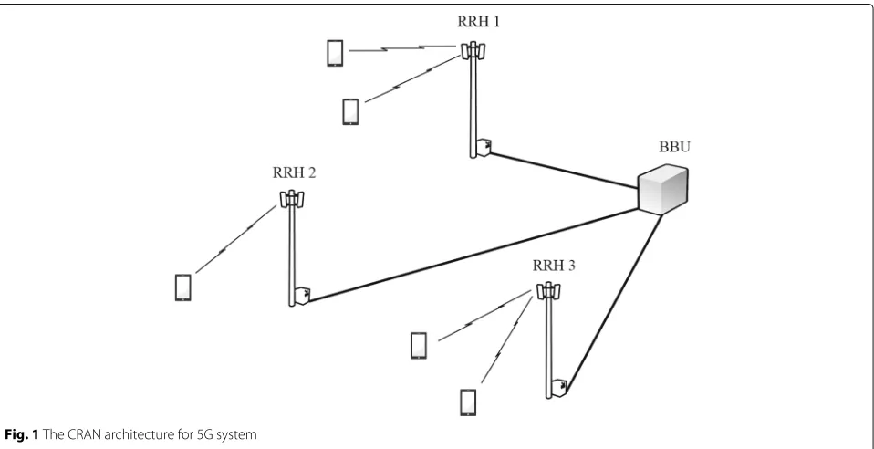
Figure 1 presents the CRAN system, consisting of the
following essential components:
• N terminals spread out across the entire CRAN system;
• A number ofR remote radio heads (RRHs) serving the terminals; and
• A baseband unit (denoted by ‘BBU’ in Fig.1) that performs baseband processing in the entire system, and to which all RRHs are connected to by a fast back-haul.
For simplicity, we consider the case where each RRH is serving only one terminal in the downlink (DL) in a given time frame. It is further assumed that the CRAN system operates in time division duplex (TDD), where
time frames of duration Tf are used for a
communica-tion link. Each time frame consists of a number of L
sub-frames, each of durationTsub. Orthogonal frequency-division multiplexing (OFDM) waveform is considered,
and therefore, each sub-frame consists of a number of symbolsStotalandfsc OFDM sub-carriers. The operating frequency of the system isfc, with a system bandwidthW. Dense deployment of RRHs is considered within the given CRAN system; an example could be placing distributed antenna systems on top of street lights [2]. Terminals are roaming freely within the area with varying velocities and directions. Each RRH and terminal is equipped withATx andARxantennas, respectively.
Finally, the following notations are followed in the description of the 5G CRAN system model and through-out the rest of this paper. Bold-faced capital letter, e.g.AAA, denotes a matrix, whereas bold-faced small letter, e.g.,aaa, denotes a vector.Adenotes a set, whereasAoradenote scalars.(.)†denotes the Hermitian of a vector or a matrix, while the transpose of a vector or a matrix is denoted by(.)T.
3.2 Resource allocation and channel model
In the considered CRAN system, the baseband unit is the central RA unit, which allocates resources on a per-frame basis. First, it performs the assignment of each RRH to the terminals present in the system. LetXXXtdenote the binary assignment matrix, where each element xtr,n denotes the assignment ofnth terminals torth RRH at timet. The assignment of the terminals to RRH, is in the literature referred to as user assignment. Once the user assignment is determined, the baseband unit decides on the selection of a transmit beamvvvt
r,nto be used by the assigned RRH,
and also the receive filteruuut
r,nat the terminal. The
trans-mit beams and receive filters belong to the pre-defined
sets of beams, i.e.,vvvt
r,n∈Vanduuutr,n∈U, that are available
at each RRH and terminal, respectively. Finally, the base-band unit selects a modulation and coding scheme (MCS),
mtr,n from the setM, for data transmission between each RRH-terminal link. The resource allocation is done by the baseband unit on per-frame basis, where the objective is to maximize the system goodput.
The propagation scenario is interference-limited, hav-ing densely deployed RRHs within the area of interest. Given a certain allocation of terminals to RRHs in the system, combined with the selection of transmit beams and receive filters for each allocation, the signal-to-interference-and-noise ratio (SINR) of a terminalnfor a given timetis given by
γnt= P
r,n is the signal power received by terminal n,
from the rth RRH, at time t, Pt
q,n is the signal power
received by terminaln, from theqth RRH (other than the
rth RRH), at the same time frame t, andσ2 is the noise power. The received signal powerPtr,nis given by
Ptr,n= PTx· |(uuutr,n)†HHHtr,nvvvtr,n|2. (2)
In Eq. (2),PTxdenotes the transmit power allocated per RRH, andHHHtr,nis the channel matrix for the time framet
between RRHrand terminaln. Throughout the duration of a frame we assume that the SINR remains constant in both time and frequency.
Each element of the channel matrixHHHtr,nrepresents the complex polarimetric channel impulse response between
each transmitter antenna element aTx and receiver
antenna elementaRx, and is denoted byHaRx,aTx(t,τ ). In reality, this channel response is the combination of dif-ferent path components, i.e., reflection, diffraction, and scattering, which can be modeled askdifferent multipath components. The channel impulse response is the sum of
the impulse responses from k different multipath
com-ponents, between aTx andaRx antenna elements and is given by
Here,K is the total number of multipath components. ˜
h h
hk,aRx,aTx(t) is the impulse response of kth multipath, including the relevant pathloss.λdenotes the wavelength, and dk is the total distance for multipath k at time t. δ(τ −τk,aRx,aTx(t))is the delta function representing the
evolution of channel impulse response with respect to different multipath delaysτk,aRx,aTx.
Given the SINR per time frame, the system utilizes the MCS mtr,n chosen by the resource allocation unit, i.e., the baseband unit, to convey backlogged informa-tion to the corresponding terminal. This results in a certain spectral efficiency combined with a block error rateemt
r,n(γ
t
n). Thus, assuming full-buffer at the baseband
unit, the choice of MCS determines a certain payload sizebmt
r,nthat can be sent over the channel, and depend-ing on the resultdepend-ing block error rate, the goodput for the corresponding link at timetcan be calculated as
Gtr,n= (1−em
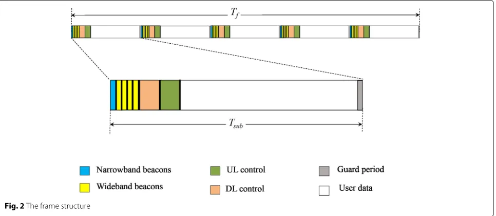
For the determination of user assignments and resource allocations, the baseband unit utilizes either the position estimates of the terminals present in the system, or their CSI. Acquisition of either of these comes at a certain sig-nalling expense, which we model as a system overhead. We assume a time frame structure, as shown in Fig. 2, where the frame duration Tf is 1 ms, and it comprises of L = 5 sub-frames, each of duration Tsub. The first few symbols of each sub-frame are used for acquiring ter-minals’ position estimates or their CSI estimates. Since TDD-based system operation is assumed, channel reci-procity holds and, therefore, the UL pilots can be used for terminals’ positions or CSI estimates in the DL subframe.
The first symbol of each sub-frame is used for posi-tion acquisiposi-tion, i.e., narrow-band pilots are sufficient for acquiring the terminals’ position estimates. The next four consecutive symbols in each sub-frame are the full-band pilots to be used for CSI acquisition. The number of pilots needed for position or CSI estimation depend on the num-ber of terminals present in the system; the greater the number of terminals, the greater the number of full-band pilots needed for CSI estimation. Typically, the number of narrow-band pilots spans a few time symbols within a frameTf. To avoid inter-carrier interference, the adjacent CSI-sensing pilots are scheduled based on the cyclic-prefix compensation distance, as explained in [2]. Also, if any of the pilots in the sub-frames within a frame are not used for position or CSI sensing, they can be used for data transmission in downlink.
Based on these parameters, the percentage overhead for position acquisition per frame can be calculated as
OHpos =
Spos·fsc,pos
Stotal·fsc,total
, (5)
Fig. 2The frame structure
beacon, and Stotal and fsc,total are the total number of OFDM symbols and sub-carriers available in the time frameTf, respectively.
Similarly, for CSI acquisition per frame, the percentage overhead can be computed as
OHCSI=
SCSI·fsc,CSI
Stotal·fsc,total
, (6)
whereSCSIandfsc,CSIdenote the number of OFDM sym-bols and the number of sub-carriers used for CSI acqui-sition of terminals present in the system in a transmitted frame, respectively.
3.4 Problem statement
The objective of this research work is to design an efficient resource allocation scheme that maximizes the sum-goodput of the CRAN based 5G system having medium- to high-speed mobility terminals. The tradi-tional approach utilizes the terminals’ CSI for doing RA in a centralized or distributed fashion for multi-antenna systems [7, 8, 17]. Certainly, the same approach can be applied for a 5G system and combined with the advantage of coordination between RRHs provided by the CRAN architecture; however, the resulting system overhead can lead to deteriorating performance for an increased num-ber of terminals in the system. In addition, the CSI-based RA approach leads to increased computational com-plexity when the number of terminals requiring service becomes large.
To alleviate these scalability problems in 5G CRAN sys-tem, we propose the usage of acquired terminals’ position estimates as an input to the RA scheme. Specifically, we design a RA scheme using machine learning algorithm to correlate the acquired terminals’ position information with different system parameters and to compare the
resulting sum-goodput with that obtained from the tra-ditional CSI-based RA scheme. Our proposed scheme is a centralized solution for resource allocation and is con-siderably less complex, but leads to other potential issues relevant to the context of using machine learning algo-rithms, namely, (a) the number of training samples for learning model needed to achieve a comparable system performance, and (b) the robustness of the learned struc-ture to changes in the live environment, which we address in this research study. In the following, we will first dis-cuss a learning-based approach which utilizes the random forests algorithm, and afterwards present a thorough per-formance evaluation.
4 Learning-based resource allocation scheme Machine learning is a tool used for making a computer program or a machine “develop new knowledge or skill from the existing and non-existing data samples to opti-mize some performance criteria” [18]. In this work, we use the random forests algorithm [11], asupervisedmachine learning technique, for designing the learning-based RA scheme. For a basic understanding of the learning approach and its application to CRAN resource allocation, a brief introduction of the random forests algorithm, fol-lowed by the details of the proposed resource allocation scheme, are presented in the remainder of this section.
4.1 Random forests algorithm
As the name suggests, the algorithm uses a combina-tion of multiple ‘random’ binary decision trees, which make up theforest, for predicting one (or a set of ) out-come(s). Being a supervised learning technique, random forests algorithm relies on provision of a training dataset to generate the decision trees. The training dataset DDD
featuresFFF, and a set of output variablesYYY. Each instance
d d
di of the training dataset is called an input feature
vec-tor. The algorithm then constructs t binary random
trees, each with a depth d, using the different
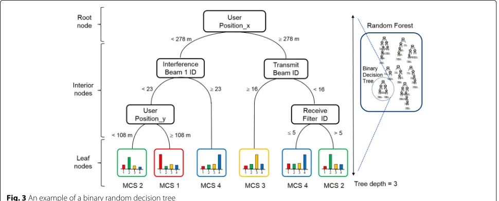
fea-tures (selected randomly) in the training dataset. Each tree typically consists of a root node, one or more inte-rior nodes and terminates at leaf nodes, as shown in the sample tree in Fig. 3. The leaf nodes store the out-put variable(s), technically called a ‘vote’, and the outout-put variable predicted by the algorithm is the mode of those votes from all trees in the random forest. It is worthy to mention here that the algorithm strives to learn the input-output correlation so as to maximize the overall accuracy of prediction, irrespective of the distribution of individual values of the output variabley. Therefore, care has to be taken that the set of output variablesYYY is not ‘biased’ toward some particular values in the training data. Once a forest has been trained (during the opera-tional phase), the input features of a new (and potentially unknown) instance is presented to the decision forest, leading to a prediction (through the voting of the trees) of the output variable. More detailed descriptions about the working of the random forests algorithm can be found in [11].
In general, random forests are known to be easy-to-use but robust machine learning data structures for noisy data. Furthermore, they can be used to calculate the ‘input variable importance,’ which signifies the influence of an input feature on prediction of the output variable. In this study, we consider system-level simulations mod-eled according to realistic scenarios, so the collected data may sometimes be noisy which will influence the over-all performance of the learning algorithm. Keeping this in view, the aforementioned properties motivated our choice
for using random forests algorithm in the design of the proposed RA scheme.
4.2 The proposed scheme
As already mentioned, the main motivation for design-ing the proposed approach is to use the acquired ter-minals’ position estimates for allocating the resources efficiently. The resources include transmit beam,vvvtr,n, per RRH-terminal link, receive filter, uuutr,n, per terminal, as well as the appropriate MCSs’ selection, mtr,n, for each RRH-terminal user assignment. We consider the case of fixed user assignments, where each RRH serves only one terminal throughout the operational phase. We apply a simplistic approach for designing the dataset to use for the training of random forests algorithm: we use the acquired terminals’ position estimates in combination with some system resources as input features, and train the algorithm for predicting the MCS as an output variable. Specifically, the input parameters, which constitute the input feature vector, are the following:
• Terminal position estimatePntof the dedicated terminal. In reality, this is acquired with certain precision using an extended Kalman filter, along with the direction of arrival and time of arrival estimates of those terminals [19].
• Transmit beamvvvtr,nused for serving the dedicated terminal. Essentially, they belong to a set of fixed beamsVbased on geometric beamforming, with a certain angular separation.
• Receive filteruuut
r,nused by the terminal to receive transmitted data in a specific direction. These filters are also geometric beams, with an angular separation dependent on the number of antennas at the terminal.
• Interfering transmit beamsvvvt
q,n,q=rused by the interfering RRHs fornth terminal.
Random forests algorithm is trained on these ‘input features’ to predict the MCS, mtr,n, such that the sum-goodput is maximized. Essentially, we deploy the random forests asmulti-class classifier, where the output variable
mtr,nhas multiple values, or classes.
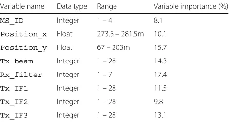
Figure3illustrates an example of a binary decision tree of depthd = 3 from a set of trees comprising a random forest. The root node comprises the input variable corre-sponding to the user position along thex-axis, while the input features corresponding to transmit beam, receive filter, interference beam for the first interfering terminal, and user position along they-axis constitute the interior nodes of the tree. A binary decision tree organizes the classification in a set of binary choices about each input in steps, starting at the root node of the tree and progressing down to the leaf nodes which represent the classifica-tion decision. At each step of the tree construcclassifica-tion, the input feature and its threshold value providing the high-est information gain are selected. An input feature and its corresponding threshold value show the highest infor-mation gain if they divide the sample training dataset in two (equally large) subsets. Table1 shows the details of the input variables used for constructing the input feature vector for training the random forests algorithm. Here, ‘Tx_IF1’ refers to the interfering transmit beam for the first interfering terminal, ‘Tx_IF2’ is the interfering
trans-mit beam for the second interferer, and so on. The leaf nodes, which corresponds to the output variable values, comprises the classification decision, i.e., the MCS indices
of which only a limited number is shown in Fig. 3 for
illustration simplicity (c.f. Table2).
It has to be noted that the organization of each trained decision tree of the random forest is determined by the bootstrap sample subset that is extracted from the train-ing dataset durtrain-ing the traintrain-ing phase. For constructtrain-ing the training dataset, we use ‘exhaustive search’ to determine the optimal allocation of resources, i.e.,vvvtr,n,uuutr,n, andmtr,n
for a terminal locationPnt, to be served by a pre-allocated
Table 1Properties of the input variables
Variable name Data type Range Variable importance (%)
MS_ID Integer 1 – 4 8.1
Position_x Float 273.5 – 281.5m 10.1
Position_y Float 67 – 203m 15.7
Tx_beam Integer 1 – 28 14.3
Rx_filter Integer 1 – 7 17.4
Tx_IF1 Integer 1 – 28 11.5
Tx_IF2 Integer 1 – 28 9.8
Tx_IF3 Integer 1 – 28 13.1
Table 2Distribution of the output variables
MCS index 1 2 3 4 5 6 7 8
Percentage distribution 28.5 0.5 1.0 1.0 0.25 1.25 4.75 62.75
RRH. In a realistic system, a heuristic approach can be used to determine the optimal resource allocation for the acquired terminal position estimates and construct the training dataset. Upon completion of the training phase, random forests is used as a ‘scheduler’ for predicting the resource variable, MCSmtr,n, for a newly acquired terminal position estimate and testing its performance. This is done by constructing a test dataset, where the newly acquired position information is compared to the known position estimates used in training dataset. The input features for the closest matching terminal position are then combined with the new position estimate to construct the test data sample, for which a prediction of MCS is obtained from the trained random forests’ data structure. Using the pre-dicted MCS, the sum-goodput is computed by combining all RRH-terminal links’ goodput, calculated using Eq.4, for evaluating the overall system performance.
Due to the inherent property of the random forests algo-rithm, this learning-based RA scheme can be expected to be robust to noisy data. Since in reality the acquired terminal position estimates can be inaccurate for some instances, the robustness property of the random forests suggests that this will not have much impact on the overall system performance. Nevertheless, in general, this robust-ness only holds up to a certain limit. In the performance evaluation section that follows, we determine these limits and discuss remedies.
5 Performance evaluation
In this research study, the performance of the random forests algorithm has been evaluated by means of simula-tion experiments. In this secsimula-tion, the simulasimula-tion assump-tions and scenarios of our evaluation methodology are first presented. This is followed by a performance analysis of the random forests algorithm providing a basis for the analysis of the performance for system level simulations. Next, a thorough analysis of various sets of performance results of the learning-based RA scheme is given in com-parison to a set of benchmark schemes. Finally, various aspects on the robustness and performance limitation of the proposed learning-based RA scheme are discussed in further detail.
5.1 Evaluation methodology
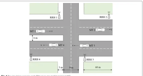
Fig. 4The simulation scenario; each RRH serves one mobile terminal (MT)
a single mobile terminal (MT). This represents a sim-pler multi-RRH, multi-terminal scenario for 5G CRAN system where only inRRH interference exists. The ter-minal position estimates can either be accurate or can be erroneous, where the error in position is modeled using normal distribution with zero mean and a given stan-dard deviation. A fixed set of transmit beams is designed using geometric beamforming, with an angular separa-tion of 3°. The receive filters are designed in the same way as the transmit beams, but the angular separation is set to 12°. Other parameter settings for the simulation set
up are given in Table 3. Assuming DL communication,
channel coefficients for each RRH-terminal link are based on TDD-based downlink and are extracted by using the map-based METIS channel model for Madrid grid [21]. A
Table 3Parameter settings
Parameter Value
fc 3.5 GHz
BW 200 MHz
RTx 8
NRx 2
hTx 10 m
hRx 1.5 m
PTx 1 mW
TTI 0.2 ms
vRx 30 m/s
ray-tracer-based channel model was implemented for this purpose, the details for which can be found in [22]. Note that in Table3,hTxrefers to the height of the RRH anten-nas, whilehRxrefers to the terminal antenna height from the ground. Finally,vRxdenotes the terminals’ velocity.
Depending on the investigation scenario (c.f., Section3), the training dataset is constructed next by using the pro-cedure outlined in Section 4. These training datasets are used to construct the multi-class Random forests model, where we rely on the implementation provided by OpenCV [23]. A total of 100 terminal positions, per ter-minal, are selected randomly from a set of 1000 terminal positions generated by Horizon, per terminal, to create training datasets of 0.25 million samples for each inves-tigation scenario. The output from the random forests model is used to compute the goodput at the terminal, referred to as user goodput, using Eq. (4). The system goodput is computed by taking the sum of the user good-put for each time instance, and its average over all con-sidered 100 terminal positions is used for system-based performance evaluation.
5.2 Performance analysis of random forests algorithm
considered 8 MCSs, in the training dataset. We notice that the output variables are concentrated more toward lower or higher MCS selection values; this is because the chan-nel gain for a particular terminal is severely influenced by the interference present in the system. Based on this observation, we need to consider an appropriate structure for constructing the random forest, such that the predic-tion of the output variable is not ‘biased’ toward the output variable value present in the majority of the training data instances in the given dataset.
In addition to the details of the input variables used for constructing the input feature vector for training the ran-dom forests algorithm, Table 1 also shows the variable importance of each input feature obtained by applying the random forests’ property, to observe its dependence on the output variable in the training dataset. From the table, it can be observed that the index of the selected receive filter beam is the most important variable that influences the value of the output variable. This is because the out-put variable, the MCS selection, is tied to the SINR value of the given terminalnfor a given time instancet, which is highly dependent on the receive filter selected to serve the usern. The terminal position is the next most important variable, which itself indicates the expected interference level seen by terminalnwhen served by a selected trans-mit beam and receive filter combination by an RRH. The interfering beam indices also considerably influence the output variable, since they are also important in decid-ing the level of interference seen by terminalnat timet. The assigned terminal ID is the least important parameter, since it only indicates the terminal considered for a given sample instance, and is loosely tied to the output variable, i.e., the MCS selected for serving the indicated terminal.
After analyzing the data characteristics, the next step is to construct and train the random forests algorithm. The training of the algorithm essentially optimizes the for-est data structure for accuracy. Here, an important aspect relates to the dimensioning of the forest itself, as it impacts the training and test accuracy. Dimensioning relates to the depth of the trees as well as the number of trees to be used in the forest. The number of random features selected for creating a node split in each tree is chosen to be√I
according to the analysis study of the random forests algo-rithm presented in [11], whereI is the number of input features.
The training accuracy is obtained by using a subset of training data for validation of the constructed random forests model. Once a sufficiently dimensioned random forest structure has been found, a test dataset is then used to compute the test accuracy of the model by pass-ing each instance of the test dataset through each of the random trees in the model. The minimum number of training samples needed to learn a given function (e.g., the resource allocation function in this case) is known as
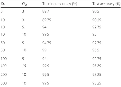
the sample complexity in statistical learning theory. As the problem is open for many functions, determining the number of training samples is usually done empirically. In this work, the number of test samples is the same as that of the training samples, i.e., 0.25 million, with 100 termi-nal positions drawn randomly from among 1000 termitermi-nal positions’ data. In terms of performance evaluation, the accuracy of the data structure built by the random forests algorithm is an important metric; the higher the num-ber of correctly predicted output variables by the model (whether for the validation dataset or the test dataset), the higher the accuracy. However, having a very high train-ing accuracy is not an indicator of an appropriate learned structure. It could be the case that the random forests structure works perfectly for the training dataset, but shows a low accuracy for test dataset. Such a structure is then an over-fit to the training data. For building a robust random forests structure, we need to vary the number of treest in the forest, as well as the depth of the trees d, in such a way that the model achieves a fairly high training accuracy while it shows good test accuracy for any test dataset with similar input feature vector compo-sition. Hence, for some data collected from a first system set-up (see the next sub-section for details), we study in Table 4 the training and test accuracy obtained for dif-ferent parametrization of the random forests structure. Based on these investigations, we used the best possible random forests model for the design of the learning-based RA scheme, with 100 trees, each with a maximum depth of 10.
Once the learned random forests structure achieves an optimal training accuracy, based on different parametriza-tion of the algorithm, it is available for predicting the output variable for the test dataset generated at run-time of the considered CRAN system.
Table 4Training and test accuracy for different parametrization of random forests model
t d Training accuracy (%) Test accuracy (%)
5 3 89.7 90.5
5.3 Evaluation results for the proposed learning-based RA scheme
We initially start with benchmarking the raw goodput for different schemes based on perfect system status knowl-edge, i.e., position or CSI. In detail, we consider the following schemes:
• The proposed learning-based RA scheme; where the multi-class random forests algorithm is used for allocating appropriate resources.
• A random MCS allocation scheme; which uses the same input features as used for the learning-based scheme, but assigns a randomly selected MCS to serve a given terminal. This scheme serves as a benchmark to directly determine the value of learning the MCS for a given input feature vector. • A geometric-based RA scheme; where the terminal
position information is used for allocating the transmit beams and receive filters for serving a given terminal, while again selecting the MCS randomly. This scheme benchmarks, in addition, the value of the pre-processing.
• A legacy CSI-based scheme; where for simplicity, we consider a scheme that determines the optimal transmit beam and receive filters based on the given CSI. This serves as an upper bound on the system performance.
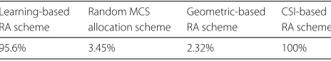
Table5presents the average system goodput for all the abovementioned comparison schemes. Note that in this investigation, we do not consider the impact from the overhead model. We initially recognize that the learning-based RA scheme achieves a performance quite close to the CSI-based scheme. In contrast, the scheme based on random MCS assignment performs a lot worse than the learning-based RA scheme, because of the spatial selec-tivity of the system. This also signifies the importance of learning the correlation between different system param-eters. The geometric-based RA scheme shows the low-est system goodput compared to the goodput obtained from the CSI-based scheme; the reason being a severely interference-limited system considered for the given case. In general, the transmit beam and receive filter selected purely on the basis of user terminal position are strictly non-optimal in an interference-limited system. Also, since the selection of MCS for serving a given terminal with known position is done at random, therefore, the system
Table 5Comparison of system goodput (in % age) for different schemes w.r.t. CSI-based RA scheme
Learning-based Random MCS Geometric-based CSI-based
RA scheme allocation scheme RA scheme RA scheme
95.6% 3.45% 2.32% 100%
goodput degrades even further. From this point onwards, we will provide a comparison of results for the proposed learning-based scheme with the CSI-based RA scheme only, since the random MCS allocation scheme as well as the geometric-based RA scheme reap off very low system goodput.
We next turn to the evaluation of the different approaches taking the system overhead into account. Since the transmitted frame duration is set to 1 ms, we assumeL=5 TDD-frames to be used for position, or CSI, acquisition and data transmission for all terminals present in the system. This serves as basic parametrization for the overhead calculations presented in Eqs.5and6. Our goal is to study the impact of overhead on performance of the learning-based and CSI-based RA schemes as the number of terminals in the system (for which the state information needs to be collected) grows. Note that we consider at this step still all state information to be perfectly accurate (i.e., the position information as well as the CSI).
Figure5shows the results of the average system good-put obtained using accurate terminal position information at all RRHs for the learning-based and CSI-based RA schemes. The colored bars show the effective average sys-tem goodput, i.e. the syssys-tem goodput obtained after taking into account the effect of system overhead due to posi-tion beaconing or CSI sensing, while the underlying gray bars represent the system performance without taking the overhead into account. Overall, the proposed learning-based RA scheme achieves about 96% of the system goodput achieved by the CSI-based scheme, without con-sidering any overhead. However, if the system overhead is accounted for, we observe that the proposed scheme is either at par or better in performance compared to the CSI-based scheme for all possible number of terminals present in the system. In particular, as we increase the number of terminals in the system, the number of narrow-band beacons for acquiring terminals’ position estimates increases gradually per TTI, and thus the overhead scales up only marginally for the learning-based RA scheme. In contrast, the overhead for the CSI-based scheme grows much stronger with the increase in the number of ter-minals present in the system, reaching up to 48% of the frame time, showing that effective system performance degrades severely if CSI-based scheme is used for resource allocation in a system with high terminal density.
Fig. 5Effect of overhead on average system goodput for different RA schemes and user terminal density, for perfect position and CSI estimates of all terminals
CSI acquisition, the learning-based RA scheme can sig-nificantly outperform CSI-based approaches (up to 100% performance improvement).
5.4 Robustness of learning-based RA scheme
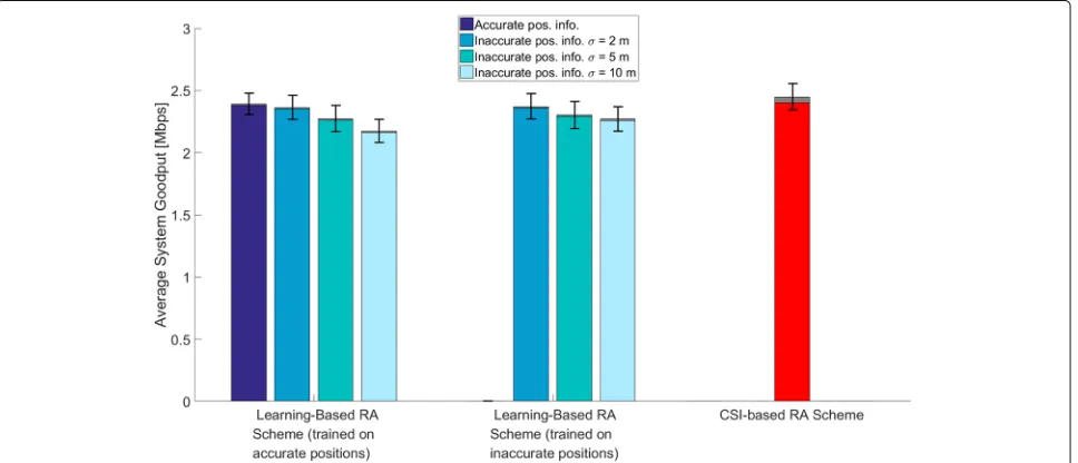
This performance advantage motivates a more thorough study on the robustness of our learning-based RA scheme. We start with considering the most obvious poten-tial source of inaccuracy influencing the learning-based scheme, namely, the accuracy of the position information. Figure6shows the results for the average system good-put obtained when a random error is involved in the position estimation for the terminals being served by RRHs. It can be seen that the classifier trained on perfect
terminal position information is enough to guarantee good system performance up to a certain degree of error involved in the position estimation. However, if the error margin in the terminal position estimates exceeds 2 m, the learning-based RA scheme trained on perfect termi-nal position estimates fails to provide satisfactory system performance. Better system goodput can be obtained by using the learning-based RA scheme trained on inaccu-rate position estimates, but the traditional CSI-based RA scheme provides still about 10% better effective system performance.
This shows the robustness of the proposed scheme for small degrees of error involved in acquired terminal position information. However, when the error margin
becomes excessively large, the CSI-based RA scheme provides better effective system performance, when the best-case terminal density scenario is considered, i.e., the scenario where the number of terminals present in the system is equal to the number of RRHs serving them.
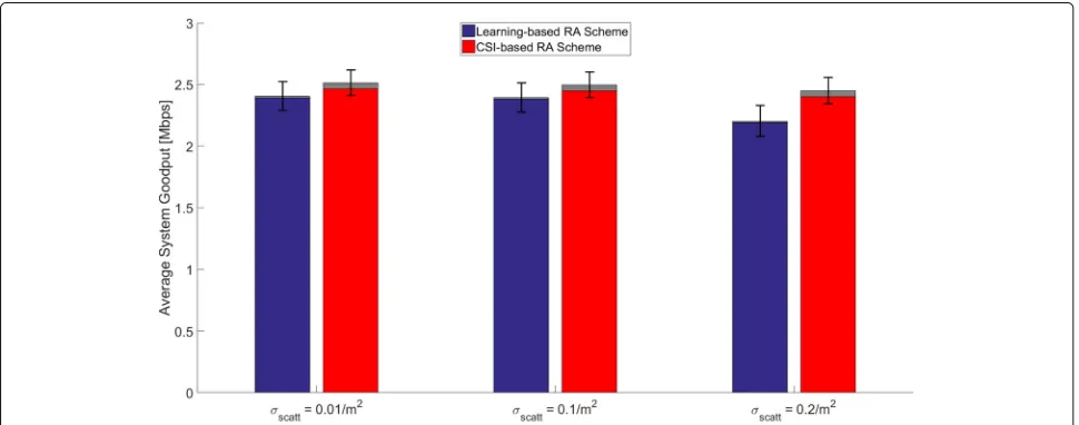
We next turn to the question how sensitive the learning-based RA scheme is to a change in the propagation scenario in contrast to the one from which the train-ing data has been acquired. Figure 7 shows the results for changing obstacle/scatterer density when the ran-dom forests model is trained only for a fixed system parameterization. We observe that the average system goodput varies only marginally with varying scatter-ers’ density ranging between 0.01 and 0.2/m2. Overall, the proposed scheme experiences only 7% loss com-pared to the traditional CSI-based RA scheme in terms of effective system goodput obtained for all considered scenarios.
5.5 Performance accuracy
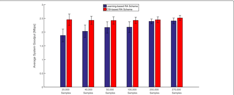
An important factor for the design of such a scheme is the quantitative analysis of the dataset, i.e., how many samples are needed to achieve a comparable system per-formance between the learning-based RA scheme and the traditional CSI-based RA scheme. For this purpose, the system-based performance with an increasing number of total samples has been computed and presented in Fig.8. More specifically, Fig.8represents the system goodput in comparison to the CSI-based scheme for different num-ber of samples used for training and testing the random forests model, without considering any overhead. These results are for the case when perfect position estimates of the users are available at each RRH, and the ran-dom forests model is trained (and tested) with the given
number of samples. For each case, the learning model has 100 trees, each with a maximum depth of 10.
As shown in Fig. 8, the performance of the learning-based RA scheme improves with greater number of samples used for training and testing; with more sam-ples comes more information about correlation between the input data features and the output variable, and thus the learning of RF model improves with increasing number of training instances with improved test accu-racy. However, the performance saturates after a cer-tain point; this happens for a total of 250,000 instances used for training and testing, in the case shown in Fig.8. Therefore, we used a total of 250,000 instances for all the abovementioned performance results’ evaluation, which is good enough to guarantee a comparable perfor-mance of the learning-based RA scheme to the CSI-based RA scheme.
5.6 Sensitivity to random antenna orientation
In the learning-based RA scheme, one of the allocated resources includes the receive filter, which is based on beamforming in the direction closest to the direction of the received signal. For this to work perfectly, it is nec-essary to have the knowledge of the terminal’s antenna orientation at the RRH serving the related terminal. The antenna orientation of the terminal defines the radiation pattern of the receiving antenna, which dictates the selec-tion of the receive filter. However, the terminal antenna orientation is typically random and can therefore be defined in the local coordinate system (LCS), whereas the terminal antenna orientation known at RRH is defined in the global coordinate system (GCS). In order to compute the correct direction of receive filter, the following trans-formation between GCS and LCS has to be used (based
Fig. 8Performance evaluation for varying number of training and test samples for the proposed learning-based RA and CSI-based RA schemes
on the discussion given in the METIS channel model documentation [21]):
FGCS(θ,φ)=
cosϕ −sinϕ
sinϕ cosϕ
Fθ,LCS(θ,φ)
Fφ,LCS(θ,φ)
. (7)
Here, FGCS represents the antenna radiation pattern in GCS,θ andφ are the elevation and azimuth angles in LCS, andFθ,LCS and Fφ,LCS denote the radiation pat-terns of terminal antenna in elevation and azimuth planes, respectively.cosϕandsinϕare the system transformation variables, given by [21]:
cosϕ=eeeθ,GCS(θ,φ)TR eeeRR θ,LCS(θ,φ), (8)
sinϕ=eeeφ,GCS(θ,φ)TR eeeRR θ,LCS(θ,φ), (9)
where,eeeθ,GCS andeeeφ,GCS are the basis vectors in GCS for elevation and azimuth planes, respectively. RRR is the rotation matrix applied for correcting the angular ori-entation in GCS based on the oriori-entation in LCS, and
eeeθ,LCS andeeeφ,LCS are the basis vectors in LCS for eleva-tion and azimuth planes, respectively. The derivaeleva-tion of the rotation matrix is given in theAppendix.
If not known a priori at the serving RRH, the antenna orientation of the user terminal is expected to affect the average system goodput. We therefore study next the impact of such a random orientation of the terminal antenna on the performance of the learning-based RA scheme. Figure9shows the effect of misalignment in ter-minal antenna orientation information in the training and test datasets for the learning-based RA scheme. It can be seen that the average system goodput is adversely affected by the misalignment in antenna orientation at the receiver, with system goodput only being about 27% of that for the traditional CSI-based scheme for resource allocation.
This is by far the biggest impact on the performance of the learning-based RA scheme found in our research work. Thus, it is important to investigate approaches to mitigate the performance degradation from random antenna orientation caused by users’ hand movements. One way to mitigate the effect of the misalignment in antenna orientation is to train the classification model for the learning-based approach using random termi-nal antenna orientation information, and then test it for dataset with random terminal antenna orientation infor-mation embedded within. This case is shown as ‘solution 1’ in Fig.9. In this case, the random terminal antenna ori-entation helps the classifier learn the correlation between different resources and terminal-related system parame-ters effectively, thus resulting in the performance gap of only 6% from the system goodput for the CSI-based RA scheme.
Another option to mitigate the effect of terminal antenna orientation is to apply a rotation matrix to adjust the predicted receive filter settings according to realistic terminal antenna orientation. The mathematical analysis for applying this solution is based on the derivation above. The performance result for this method is shown in Fig.9 by the bar labeled ‘solution 2.’ In this case, we achieve almost 85% of the average system goodput compared to the CSI-based scheme, which is fairly good but worse than the performance seen for ‘solution 1.’ A possible reason for this performance loss is the interference present in the system, which makes the solution of only rotating the predicted receive filter for good reception at terminal a sub-optimal approach.
Fig. 9Effect of misalignment in terminal antenna orientation on the average system goodput and its mitigation results
additional signalling from the terminal to the baseband unit, for which we do not here account for the overhead. The performance of this approach is shown as ‘solution 3’ in Fig. 9, where we observe that the performance of the proposed technique reaps off almost the same average sys-tem goodput as in case of ‘solution 1.’ Since we use the same number of features for random selection in building the decision trees in random forests model, the random-ization of trees in the model results in the variation of the obtained system goodput, for the case when terminal antenna orientation is embedded or is exclusively incor-porated as an input feature for training the random forests model, i.e., for ‘solution 1’ and ‘solution 3,’ respectively. We conclude with the remarkable observation that the random antenna orientation can basically deteriorate per-formance strongly; however, especially by including this effect in the training data, more robust MCS selections can be trained to compensate for this randomness.
5.7 Change in channel statistics
A special case for testing the performance of the pro-posed scheme is when the LOS links are no more exis-tent between the RRHs and the relevant terminals in the system. In this case, the specular component is totally neglected when computing the channel matrix for a given RRH-terminal link, thus resulting in a non-LOS (NLOS)
scenario. Figure 10 shows the average system goodput
obtained from the proposed learning-based, as well as the traditional CSI-based RA schemes, for different inac-curacy ranges involved in the acquired terminal position estimates. We kept the range of terminal position inac-curacy fairly small in this case, since NLOS consideration is already enough to result in performance degrada-tion using only terminal-posidegrada-tion estimates for resource allocation in the system. Overall, for perfect terminal position information availability, the proposed scheme still performs fairly well, reaping off almost 90% of the
system goodput obtained using CSI-based RA scheme. The effects on average system performance for differ-ent variation in terminal position inaccuracies do not show a specific trend, because of the changing chan-nel statistics in NLOS scenario. However, training on inaccurate terminal position estimates proves to be ben-eficial in improving the system goodput, in contrast to the effect seen in LOS case, where the learning-based scheme trained only on perfect terminal position infor-mation is enough to guarantee a system performance comparable to the traditional CSI-based RA scheme, when lower accuracy is involved in the terminals’ position estimates.
6 Conclusions
We presented the design of a learning-based RA scheme which has much lower system overhead, as well as lower complexity, than the traditionally used CSI-based RA scheme, because of its dependence on only the acquired terminal position estimates. Random forests algorithm is used for designing learning-based RA scheme, that works as a scheduler for appropriate resource allocation in 5G CRAN system, serving the different terminals using only their position information. A comparison analysis was done for the RA scheme based on random forests model and the CSI-based RA scheme, in different contexts. The proposed scheme shows either comparable or signifi-cantly better effective system performance compared to the CSI-based RA scheme for different terminal densities in the system. In terms of the design parameter variations, the proposed scheme is fairly robust to the inaccuracy involved in the terminal position estimation. Training the random forests model on the dataset involving variation in either the system metrics or the design parameters for the learning-based scheme is very beneficial in case when the same model trained on fixed system parametrization shows degraded system performance. In general, for LOS or NLOS cases, the proposed scheme is robust to small error margin involved in the acquired terminal position information, as well as to the variation in system char-acterization (such as changing scatterers’ density). The change in terminal antenna orientation affects the per-formance of the proposed scheme most severely, but the effect can be mitigated by training on top of the termi-nal antenna orientation information, either embedded or provided explicitly in the training data for constructing the random forest. The performance limitations of the learning-based scheme for extreme channel characteriza-tion variacharacteriza-tion is still an open quescharacteriza-tion, which will be a part of the future work. Also, the scope of the proposed scheme is limited to a centralized solution for resource alloca-tion in CRAN-based 5G systems. Designing a similar learning-based RA scheme as a distributed solution for CRAN architecture, with the interference coordination
between the baseband units, is a potential topic for future research.
Appendix
This appendix presents a derivation for the rotation matrix. The basic rotation matrices for rotating the vec-tors by an angle inx-,y-, orz-axes using the right-hand
For the pre-defined orientation angles of the receive fil-ter for a fil-terminal, the rotation matrix can be computed as:
R R
R=RRRz(φ0)RRRy(θ0). (13)
Expanding the above expression, we get the following form:
Inserting this rotation matrix expression in Eq.8results in the following expressions forcosϕandsinϕ:
cosϕ=cosθcosφcosθ sinφ −sinθRRR
Simplifying these matrix multiplications gives
Abbreviations
5G: 5th generation; BBU: Baseband unit; CRAN: Cloud radio access network; CSI: Channel state information; D2D: Device-to-device; DL: Downlink; GCS: Global coordinate system; IoT: Internet of things; KPI: Key performance indicator; LCS: Local coordinate system; LOS: Line-of-sight; LTE: Long-term evolution; LTE-A: Long-term evolution-advanced; MIMO: Multiple-input multiple-output; MCS: Modulation and coding scheme; MT: Mobile terminal; NLOS: Non-line-of-sight; OFDM: Orthogonal frequency-division multiplexing; RA: Resource allocation; RAN: Radio access network; RRH: Remote radio head; SINR: Signal-to-interference-and-noise ratio; TDD: Time division duplex; TTI: Time transmission interval; UDN: Ultra-dense network; UL: Uplink
Acknowledgements
The authors would like to thank Mr. Christer Qvarfordt and Dr. Kari Leppänen both with Huawei Technologies for valuable discussions.
Competing interests
The authors declare that they have no competing interests.
Publisher’s Note
Springer Nature remains neutral with regard to jurisdictional claims in published maps and institutional affiliations.
Author details
1Department of Information Science and Engineering, KTH Royal Institute of
Technology, Osquldas väg 10, SE-10044 Stockholm, Sweden.2Radio Network Technology, Huawei Technologies Sweden AB, Skalholtsgatan 9, SE-16494 Kista, Stockholm, Sweden.
Received: 16 January 2018 Accepted: 11 May 2018
References
1. QC Li, H Niu, AT Papathanassiou, G Wu, 5G Network capacity: key elements and technologies. IEEE Veh. Technol. Mag.9(1), 71–78 (2014). https://doi.org/10.1109/MVT.2013.2295070
2. P Kela, J Turkka, M Costa, Borderless mobility in 5G outdoor ultra-dense networks. IEEE Access.3, 1462–1476 (2015).https://doi.org/10.1109/ ACCESS.2015.2470532
3. S Imtiaz, H Ghauch, MMU Rahman, G Koudouridis, J Gross, in
Learning-Based Resource Allocation Scheme for TDD-Based 5G CRAN System. Proceedings of the 19th ACM International Conference on Modeling, Analysis and Simulation of Wireless and Mobile Systems. MSWiM ’16 (ACM, New York, 2016), pp. 176–185.https://doi.org/10.1145/2988287.2989158 4. JG Andrews, S Buzzi, W Choi, SV Hanly, A Lozano, ACK Soong, JG Zhang,
What will 5G be?. IEEE J. Sel. Areas Commun.32(6), 1065–1082 (2014) 5. M Hadzialic, B Dosenovic, M Dzaferagic, J Musovic, inCloud-RAN:
Innovative Radio Access Network Architecture. Proceedings ELMAR-2013 (IEEE, 2013), pp. 115–120
6. N NGMN, 5G White Paper. tech. rep. 2015 (2015). Available:https://www. ngmn.org/fileadmin/ngmn/content/downloads/Technical/2015/NGMN_ 5G_White_Paper_V1_0.pdf. Accessed 26 May 2018
7. TE Bogale, L Vandendorpe, Weighted sum rate optimization for downlink multiuser mimo coordinated base station systems: Centralized and distributed algorithms. IEEE Trans. Sign. Process.60(4), 1876–1889 (2012). https://doi.org/10.1109/TSP.2011.2179538
8. A Chiumento, C Desset, S Pollin, LV der Perre, R Lauwereins, Impact of CSI Feedback Strategies on LTE Downlink and Reinforcement Learning Solutions for Optimal Allocation. IEEE Trans. Veh. Technol.66(1), 550–562 (2017).https://doi.org/10.1109/TVT.2016.2531291
9. JC Shen, J Zhang, KC Chen, KB Letaief, High-dimensional CSI acquisition in massive MIMO: sparsity-inspired approaches. IEEE Systems Journal.11(1), 32–40 (2017).http://dx.doi.org/10.1109/JSYST.2015.2448661
10. M Botsov, S Sta ´nczak, P Fertl, inComparison of Location-based and CSI-based Resource Allocation in D2D-Enabled Cellular Networks. 2015 IEEE International Conference on Communications (ICC), (2015),
pp. 2529–2534.https://doi.org/10.1109/ICC.2015.7248705 11. L Breiman, Random forests. Mach. Learn.45(1), 5–32 (2001)
12. HZ O. Punal, J Gross, inRFRA: Random Forests Rate Adaptation for Vehicular Networks. Proc. of the 13th IEEE International Symposium on a World of
Wireless, Mobile and Multimedia Networks 2013 (WoWMoM 2013) (IEEE, 2013)
13. M Vincenzi, A Antonopoulos, E Kartsakli, J Vardakas, L Alonso, C Verikoukis, Multi-tenant slicing for spectrum management on the road to 5g. IEEE Wirel. Commun.24(5), 118–125 (2017).https://doi.org/10.1109/MWC. 2017.17001388088538
14. E Datsika, A Antonopoulos, N Zorba, C Verikoukis, Software defined network service chaining for ott service providers in 5g networks. IEEE Wirel. Commun.55(11), 124–131 (2017).https://doi.org/10.1109/MCOM. 2017.1700108. 8114562
15. MY Lyazidi, N Aitsaadi, R Langar, inResource Allocation and Admission Control in OFDMA-Based Cloud-RAN. 2016 IEEE Global Communications Conference (GLOBECOM), (2016), pp. 1–6.https://doi.org/10.1109/ GLOCOM.2016.7842217
16. JP Leite, PHP de Carvalho, RD Vieira, inA flexible framework based on reinforcement learning for adaptive modulation and coding in OFDM Wireless Systems. 2012 IEEE Wireless Communications and Networking Conference (WCNC), (2012), pp. 809–814.https://doi.org/10.1109/WCNC. 2012.6214482
17. X Wang, P Zhu, FC Zheng, C Meng, X You, inEnergy-efficient resource allocation in multi-cell OFDMA systems with imperfect CSI. 2015 IEEE 82nd Vehicular Technology Conference (VTC2015-Fall), (2015), pp. 1–5.https:// doi.org/10.1109/VTCFall.2015.7390923
18. E Alpaydin,Introduction to machine learning. (MIT press, Cambridge, 2014) 19. J Werner, M Costa, A Hakkarainen, K Leppänen, M Valkama, inJoint User
Node Positioning and Clock Offset Estimation in 5G Ultra-Dense Networks. 2015 IEEE Global Communications Conference (GLOBECOM), (2015), pp. 1–7.https://doi.org/10.1109/GLOCOM.2015.7417360
20. G Kunz, O Landsiedel, S Götz, K Wehrle, J Gross, F Naghibi, inExpanding the Event Horizon in Parallelized Network Simulations. Modeling, Analysis & Simulation of Computer and Telecommunication Systems (MASCOTS), 2010 IEEE International Symposium On (IEEE, 2010), pp. 172–181 21. V Nurmela, A Karttunen, A Roivainen, L Raschkowski, T Imai, J Järveläinen,
J Medbo, J Vihriälä, J Meinilä, J Kyröläinen, K Haneda, V Hovinen, J Ylitalo, N Omaki, V-M Kolmonen, T Jämsä, P Kyösti, K Kusume,METIS D1.2: Initial channel models based on measurements, (2014)
22. P Kela,et al, inLocation Based Beamforming in 5G Ultra-Dense Networks. Proc. Vehicular Technology Conference (VTC Fall), 2016 IEEE 84th (IEEE, 2016). accepted for publication
23. K Pulli, A Baksheev, K Kornyakov, V Eruhimov, Real-time Computer Vision with OpenCV. Commun. ACM.55(6), 61–69 (2012).http://doi.acm.org/10. 1145/2184319.2184337