Scalable Methods for Uncertainty Quantification, Data Assimilation and Target Accuracy Assessment for Multi-Physics Advanced Simulation of Light Water Reactors.

ABSTRACT

KHUWAILEH, BASSAM ABDULLAH AYED. Scalable Methods for Uncertainty Quantification, Data Assimilation and Target Accuracy Assessment for Multi-Physics Advanced Simulation of Light Water Reactors. (Under the direction of Dr. Paul. J. Turinsky). High fidelity simulation of nuclear reactors entails large scale applications characterized with high dimensionality and tremendous complexity where various physics models are integrated in the form of coupled models (e.g. neutronic with thermal-hydraulic feedback). Each of the coupled modules represents a high fidelity formulation of the first principles governing the physics of interest. Therefore, new developments in high fidelity multi-physics simulation and the corresponding sensitivity/uncertainty quantification analysis are paramount to the development and competitiveness of reactors achieved through enhanced understanding of the design and safety margins. Accordingly, this dissertation introduces efficient and scalable algorithms for performing efficient Uncertainty Quantification (UQ), Data Assimilation (DA) and Target Accuracy Assessment (TAA) for large scale, multi-physics reactor design and safety problems.

Once the elite set of DoF is determined, the uncertainty/sensitivity/target accuracy assessment and data assimilation analysis can be performed accurately and efficiently for large scale, high dimensional multi-physics nuclear engineering applications. Hence, in this work a Karhunen-Loève (KL) based algorithm previously developed to quantify the uncertainty for single physics models is extended for large scale multi-physics coupled problems with feedback effect. Moreover, a non-linear surrogate based UQ approach is developed, used and compared to performance of the KL approach and brute force Monte Carlo (MC) approach.

On the other hand, an efficient Data Assimilation (DA) algorithm is developed to assess information about model’s parameters: nuclear data cross-sections and thermal-hydraulics

parameters. Two improvements are introduced in order to perform DA on the high dimensional problems. First, a goal-oriented surrogate model can be used to replace the original models in the depletion sequence (MPACT – COBRA-TF - ORIGEN). Second, approximating the complex and high dimensional solution space with a lower dimensional subspace makes the sampling process necessary for DA possible for high dimensional problems.

Moreover, safety analysis and design optimization depend on the accurate prediction of various reactor attributes. Predictions can be enhanced by reducing the uncertainty associated with the attributes of interest. Accordingly, an inverse problem can be defined and solved to assess the contributions from sources of uncertainty; and experimental effort can be subsequently directed to further improve the uncertainty associated with these sources. In this dissertation a subspace-based gradient-free and nonlinear algorithm for inverse uncertainty quantification namely the Target Accuracy Assessment (TAA) has been developed and tested.

Scalable Methods for Uncertainty Quantification, Data Assimilation and Target Accuracy Assessment for Multi-Physics Advanced Simulation of Light Water Reactors

by

Bassam Khuwaileh

A dissertation submitted to the Graduate Faculty of North Carolina State University

in partial fulfillment of the requirements for the Degree of

Doctor of Philosophy

Nuclear Engineering

Raleigh, North Carolina 2015

APPROVED BY:

_______________________________ ______________________________

Dr. Paul J. Turinsky Dr. Ralph C. Smith

Committee Chair

________________________________ ________________________________

DEDICATION

In loving memory of my late grandfather Ayed Khuwaileh who filled my life with grace and wisdom. My greater sorrow is being and will forever be that I never had the chance to say a final good bye. Grandfather: you shall not be forgotten.

To the soul of Captain Muath Al-Kasasbeh who martyred defending our beloved Jordan. Captain: though we never met, and now never shall, your bravery and sacrifice will be forever engraved in our hearts.

Finally, to my father Dr. Abdullah Khuwaileh, mother Entesar Al-Dawood for their endless support and motivation. To my brother Tarik Khuwaileh who has been and will forever be my best friend. To my lovely sisters Rawan and Difaf and brothers Hamzah and Baker and everybody in my beloved Ramtha.

ii BIOGRAPHY

Bassam Abdullah Khuwaileh, born in Ramtha, Jordan on July 19th _{1989 to Abdullah}

Khuwaileh (a university professor) and Entisar Al-Dawood (a school teacher). He received his elementary and secondary education in Ramtha, graduating from Ramtha High School in 2007 with honor.

iii ACKNOWLEDGMENTS

My utmost and most sincere gratitude to my advisor, Prof. Paul J. Turinsky for the continuous support of my Ph.D study and related research, for his patience, motivation, and immense knowledge. His guidance helped me in all the time of research and writing of this dissertation.

Besides my advisor, my appreciation goes to my doctoral committee: Dr. Nam T. Dinh, Dr. Ugur Mertyurek and Dr. Ralph C. Smith for their insightful comments and encouragement. My sincere thanks also goes to Dr. Hany S. Abdel-Khalik, Dr.Youngsuk Bang, and Dr.Congjian Wang whom their help and collaborations was so precious. Also, I would like to thank Oak Ridge National laboratory and more specifically Dr. Goran Arbanas and Dr. Mark Williams who provided me an opportunity to join their team. Thanks for Texas Advanced Computing Center for offering the computer allocation required to perform a large part of this research without their precious support it would not be possible to conduct considerable part of this research. Also, I would like to thank the Consortium for Advanced Simulation of Light Water Reactors (CASL) and the U.S. Department of Energy for supporting this research.

iv TABLE OF CONTENTS

LIST OF TABLES ... vii

LIST OF FIGURES ... x

CHAPTER 1.INTRODUCTION ... 1

1.1 Motivation ... 3

1.2 Uncertainty Quantification ... 7

1.3 Data Assimilation ... 10

1.4 Inverse Uncertainty Quantification (Target Accuracy Assessment) ... 14

1.5 Reduced Order Modeling ... 17

1.5.1 Overview ... 17

1.5.2 Reduced Order Modeling Based Sensitivity Analysis, Uncertainty Quantification and Data Assimilation ... 21

1.5.3 Reduced Order Modeling Based Goal-Oriented Surrogate Construction... 27

1.6 SCALE ... 30

1.6.1 TRITON ... 31

1.6.2 NEWT ... 33

1.6.3 ORIGEN ... 35

1.7 VERA-CS ... 36

1.7.1 MPACT ... 37

1.7.2 COBRA-TF ... 40

CHAPTER 2.EFFICIENT SUBSPACE APPROXIMATION FOR SINGLE PHYSICS MODELS………. ... 45

v

2.2 Numerical Test: Lattice Physics ... 60

2.3 Numerical Test: 3-Dimensional Assembly Model Calculations ... 71

CHAPTER 3. EFFICIENT SUBSPACE APPROXIMATION FOR MULTI-PHYSICS COUPLED MODELS WITH FEEDBACK ... 77

3.1 Gradient-Based Multi-Physics Range Finding Algorithm ... 80

3.1.1 Case Study: CASL Progression Problem 2 – lattice. ... 86

3.2 Gradient-Free Multi-Physics Range Finding Algorithm ... 92

3.2.1 Case Study: Gradient-Free vs. Gradient-Based. ... 97

3.3 Case Study: 3-D Depletion Problem with Thermal-Hydraulics Feedback. ... 98

CHAPTER 4.EFFICIENT MULTI-PHYSICS UNCERTAINTY QUANTIFICATION…... 101

4.1 Efficient Uncertainty Quantification for Single Physics ... 103

4.2 Efficient Sensitivity Analysis ... 106

4.3 Efficient Uncertainty Quantification for Multi-Physics Coupled Models ... 108

4.4 Case Study: Lattice Assembly Depletion (CASL Progression Problem 2) ... 112

4.5 Case Study: Efficient Uncertainty Quantification for 3-D Assembly Depletion with Thermal-Hydraulics Feedback ... 113

4.6 Case Study: Efficient Uncertainty Quantification for 3-D Core Depletion with Thermal-Hydraulics Feedback (CASL Progression Problem 9) ... 141

CHAPTER 5.SURROGATE BASED DATA ASSIMILATION FOR PRESSURIZED WATER REACTORS ... 157

vi 5.2 Case Study: Efficient Data Assimilation for 3-Dimensional Core Wide Depletion

with Thermal-Hydraulics Feedback. CASL Progression Problem 9. ... 174

CHAPTER 6.TARGET ACCURACY ASSESSMENT FOR HIGH DIMENSIONAL LIGHT WATER REACTOR SIMULATION PROBLEMS ... 184

6.1 Regularization of the Inverse Uncertainty Quantification Problem ... 186

6.1.1 Algorithm ... 190

6.1.2 Case Study: CASL Progression Problem 2 – Lattice Model ... 196

6.2 Inverse Uncertainty Quantification for High Dimensional Constrained Problems 204 6.2.1 Algorithm ... 205

6.2.2 Case Study: High Dimensional Single Physics Target Accuracy Assessment– Lattice/Depletion... 208

6.3 Multi-Physics Target Accuracy Assessment ... 215

6.3.1 Algorithm ... 217

6.3.2 Case Study: CASL Progression Problem 2 – Lattice/Depletion ... 223

6.3.3 Case Study: Target Accuracy Assessment for 3-D Assembly Depletion Problem (CASL Progression Problem 6) ... 229

CHAPTER 7.SUMMARY, CONCLUSIONS AND RECOMMENDATIONS ... 234

REFERENCES… ... 239

APPENDICES… ... 251

Appendix A ... 252

vii

LIST OF TABLES

Table 1. Computational costs required for constructing the N-subspace and C-subspace. .... 64

Table 2. CASL Problem 6 Specifications [67]. ... 73

Table 3. Stopping criteria for VERA-CS analysis of 3D assembly. ... 75

Table 4. Error in k_effdue to cross-section approximation using Eq.(36) ... 91

Table 5.Uncertainty propagation via the MP-EUQ. ... 113

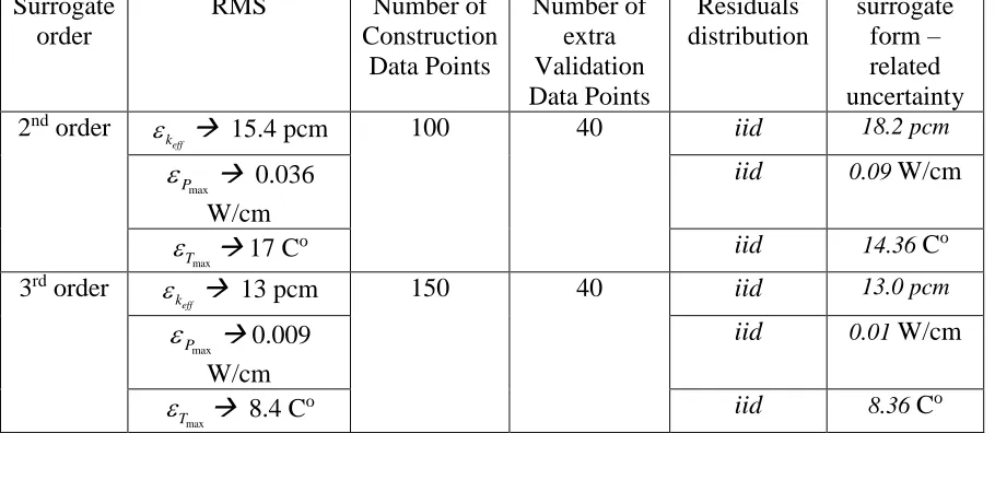
Table 6. Features of the Surrogate. ... 126

Table 7. Summary of the k-eff uncertainty results – joint parameters (MCUQ vs. MP-EUQ vs. SBUQ) ... 136

Table 8. Summary of the Maximum Pin Power uncertainty results – joint parameters (MCUQ vs. MP-EUQ vs. SBUQ). ... 138

Table 9. Summary of the Maximum Pin Temperature uncertainty results – joint parameters (MCUQ vs. MP-EUQ vs. SBUQ). ... 140

Table 10. Problem 9 features and design properties. ... 144

Table 11. Features of the Surrogate. ... 145

Table 12. Summary of the keff uncertainty results – joint parameters (MCUQ vs. MP-EUQ vs. SBUQ)... 154

Table 13. Summary of the Maximum Pin Power uncertainty results – joint parameters (MCUQ vs. MP-EUQ vs. SBUQ). ... 155

Table 14. Summary of the Maximum Pin Temperature uncertainty results – joint parameters (MCUQ vs. MP-EUQ vs. SBUQ). ... 156

Table 15. Surrogate features. ... 170

viii

Table 17. 47 group structure. ... 172

Table 18. Assimilation performance measure for the various cross-sections parameters being calibrated. ... 173

Table 19. Data assimilation results for a few important parameters... 174

Table 20. Surrogate features. ... 180

Table 21. Measurements and their uncertainties... 180

Table 22. Assimilation performance measure for the various cross-sections parameters being calibrated. ... 182

Table 23. Data assimilation results for a few important parameters... 183

Table 24.Summary of the numerical results and comparison of the two algorithms. ... 199

Table 25. Summary of the results. The 10 most affected reactions: IUQ algorithm. ... 201

Table 26. Summary of the results. The 10 most affected reactions: SIUQ algorithm. ... 202

Table 27. Identifiability test - Full dimensional space analysis. ... 203

Table 28. Identifiability test - Reduced dimensional space analysis (SIUQ algorithm). ... 204

Table 29. Summary of the results. ... 212

Table 30.The required experiments along with the required uncertainties. ... 213

Table 31. Uncertainty in the multiplication factor. ... 213

Table 32. Summary of the numerical results and comparison of the two algorithms. ... 228

Table 33. The experimental requirements along with their required uncertainties – (EoC). 228 Table 34. The experimental requirements along with their required uncertainties – (BoC). 229 Table 35. Initial and target accuracies for the responses of interest. ... 232

x

LIST OF FIGURES

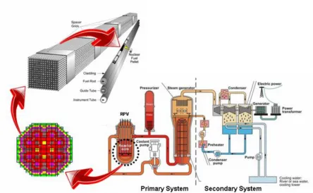
Figure 1. Nuclear Reactor

(http://energy.gov/articles/modeling-and-simulation-nuclear-reactors-hub ). ... 3

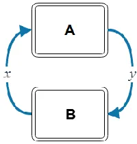
Figure 2. Two coupled multi-physics models. ... 5

Figure 3. Two serially coupled models. ... 22

Figure 4. Original model: with high dimensional input space and high computational cost. . 30

Figure 5. Goal oriented surrogate model: with few parameters and low computational cost. 30 Figure 6. Depletion with thermal-hydraulics feedback using VERA-CS (Predictor-corrector method). ... 37

Figure 7. 3-dimensional cylindrical geometry (system volume V). ... 39

Figure 8. 3-dimensional rectangular geometry (system volume V). ... 39

Figure 9. Algorithm schematic for: (a). C-Subspace (b). N-subspace. ... 52

Figure 10. ERFA flow char. ... 59

Figure 11. (a) PWR quarter fuel lattice. (b) BWR fuel lattice. ... 62

Figure 12. Error in the flux as obtained from the N-subspace vs. the C-subspace (PWR). ... 63

Figure 13. Error in the flux as obtained from the N-subspace vs. the C-subspace (BWR). ... 63

Figure 14. The dominant angle reduction as the rank increases (PWR). ... 65

Figure 15. Eigenvalue errors for the N- and. the C-subspace. ... 69

Figure 16. The eigenvalue errors for the C-subspace (1st order vs. 2nd order). ... 69

Figure 17. The eigenvalue errors for the N-subspace (1st order vs. 2nd order). ... 70

Figure 18. The flux errors for the EPGPT’s C-subspace (1st order vs. 2nd order). ... 70

xi Figure 20. Error in the L2 norm of the 3-D pin power distribution (the N-subspace vs. the

C-subspace). Refer to Eq.(32). ... 76

Figure 21. A schematic of coupled models. ... 79

Figure 22 . GB-MPRFA flow diagram. ... 83

Figure 22. Illustration example. ... 85

Figure 23. Transport model (Physics A) coupled with depletion model (Physics B)... 87

Figure 24. CASL Progression Problem number 2 – lattice. ... 88

Figure 26. Single-Physics vs. Multi-Physics Active Subspace ( ). ... 89

Figure 27. Cross section subspace as obtained from the single physics examination compared to the one obtained from the multi-physics examination (). ... 90

Figure 28.GF-MPRFA flow diagram. ... 96

Figure 29. CASL VERA problem number 1 simulated using SCALE6.1... 98

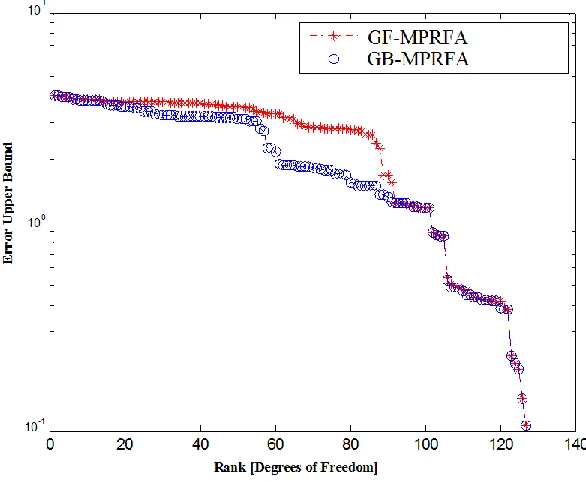
Figure 30. GB-MPRFA vs. GF-MPRFA ... 98

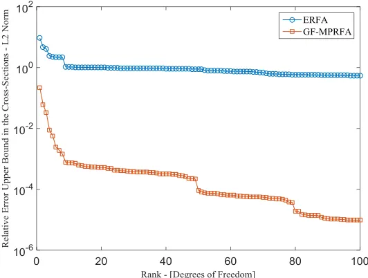
Figure 29. GF-MPRFA vs. ERFA. ... 100

Figure 30. The error upper bound in the 2-norm of the cross-section vector due to representing the lower dimensional subspace approximation of the cross-sections space. .. 113

Figure 31. Assembly Configuration. ... 120

Figure 32. A flow chart illustrating the series of coupled models in VERA-CS Depletion with thermal-hydraulics feedback. ... 120

xii Figure 34. Residuals in predicting the maximum pin power (

max

P

 ) for a range of the gap

conductivity and cross-sections (hgap , kcond and ) for 40 samples (surrogate vs. VERA-CS). ... 127

Figure 35. Residuals in predicting the maximum pin temperature (

max

T

 )for a range of the gap

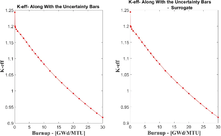
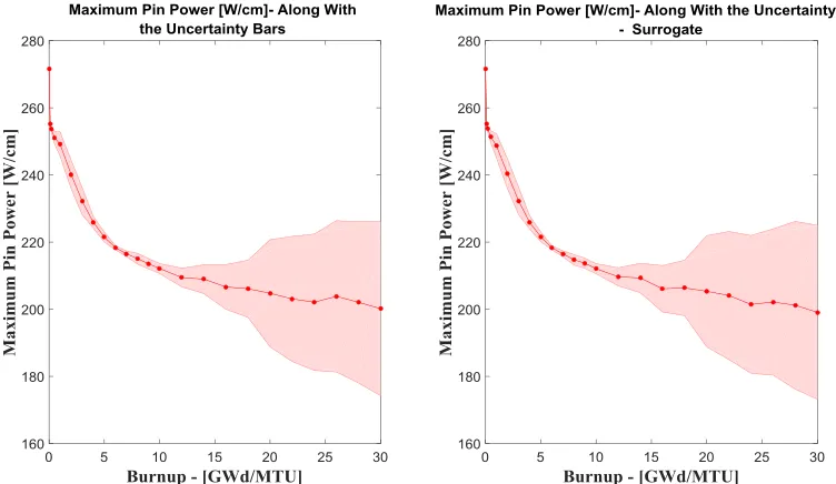
conductivity and cross-sections (hgap , kcond and ) for 40 samples (surrogate vs. VERA-CS). ... 127 Figure 36. Burnup dependent keff along with uncertainty ±σ due to the gap conductivity. .. 128 Figure 37. Burnup dependent keff along with uncertainty ±σ due to the fuel thermal

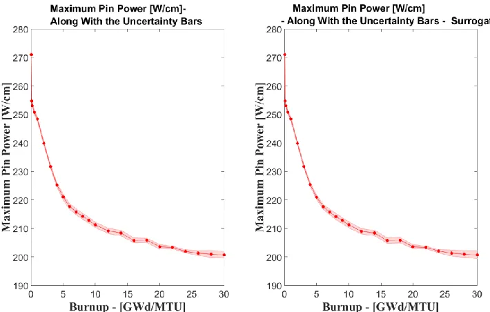
conductivity... 128 Figure 38. Burnup dependent maximum pin power along with uncertainty ±σ due to the gap

conductivity... 129 Figure 39. Burnup dependent maximum pin power along with uncertainty ±σ due to the fuel

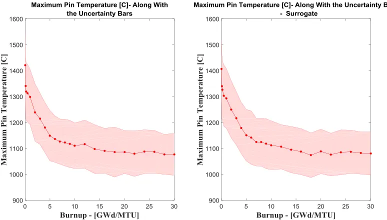
thermal conductivity. ... 129 Figure 40. Burnup dependent maximum pin temperature along with uncertainty ±σ due to the

fuel thermal conductivity. ... 130 Figure 41. Burnup dependent maximum pin temperature along with uncertainty ±σ due to the

gap conductivity. ... 130 Figure 42. Burnup dependent keff along with uncertainty ±σ due to the nuclear data cross-sections. ... 131 Figure 43. Burnup dependent maximum pin power along with uncertainty ±σ due to the

xiii Figure 44. Burnup dependent maximum pin temperature along with uncertainty ±σ due to the

nuclear data cross-sections uncertainty. ... 132 Figure 45. Burnup dependent keff along with uncertainty ±σ due to the grid-loss coefficient uncertainty... 132 Figure 46. Burnup dependent maximum pin power along with uncertainty ±σ due to the

grid-loss coefficient uncertainty. ... 133 Figure 47. Burnup dependent maximum pin temperature along with uncertainty ±σ due to the

grid-loss coefficient uncertainty. ... 133 Figure 48. Burnup dependent keff along with uncertainty ±σ due to joint samples. ... 134 Figure 49. Burnup dependent maximum pin power along with uncertainty ±σ due to joint

samples. ... 134 Figure 50. Burnup dependent maximum pin temperature along with uncertainty ±σ due to

joint samples ... 135 Figure 51. Core layout in quarter symmetry [58]. ... 145 Figure 52. Residuals in predicting the keff (

eff k

 ) for a range of the gap conductivity and

cross-sections (hgap and ) for 30 samples (surrogate vs. VERA-CS). ... 146 Figure 53. Residuals in predicting the maximum pin power (

max

P

 ) for a range of the gap

conductivity and cross-sections (hgap and ) for 30 samples (surrogate vs. VERA-CS). ... 146 Figure 54. Residuals in predicting the maximum pin temperature (

max

T

 ) for a range of the gap

xiv Figure 56. Burnup dependent maximum pin power along with uncertainty ±σ due to the gap

conductivity... 148 Figure 57. Burnup dependent maximum pin temperature along with uncertainty ±σ due to the

gap conductivity. ... 148 Figure 58. Burnup dependent keff along with uncertainty ±σ due to the nuclear data cross-sections. ... 149 Figure 59. Burnup dependent maximum pin power along with uncertainty ±σ due to the

nuclear data cross-sections. ... 149 Figure 60. Burnup dependent maximum pin temperature along with uncertainty ±σ due to the

nuclear data cross-sections uncertainty. ... 150 Figure 61. Burnup dependent keff along with uncertainty ±σ due to the grid-loss coefficient uncertainty... 150 Figure 62. Burnup dependent maximum pin power along with uncertainty ±σ due to the

grid-loss coefficient uncertainty. ... 151 Figure 63. Burnup dependent maximum pin temperature along with uncertainty ±σ due to the

grid-loss coefficient uncertainty. ... 151 Figure 64. Burnup dependent keff along with uncertainty ±σ due to joint samples. ... 152 Figure 65. Burnup dependent maximum pin power along with uncertainty ±σ due to joint

samples. ... 152 Figure 66. Burnup dependent maximum pin temperature along with uncertainty ±σ due to

xv Figure 69. Residual errors along with their distribution – Outlet Coolant Temperature (T_outlet). ... 167

Figure 70. Residual errors along with their distribution – Inlet Coolant Temperature (T_inlet). ... 168

Figure 71. Chain and posterior distribution of the grid loss coefficient (g_loss). ... 168

Figure 72. Chain and posterior distribution of the gap conductivity (h_gap). ... 169

Figure 73. Correlation between the gap conductivity (h_gap) and the grid loss coefficient (g_loss

). ... 169 Figure 74. Residual errors along with their distribution - keff ... 177 Figure 75. Residual errors along with their distribution – Fission Rate at the core center. .. 178

Figure 76. Chain and posterior distribution of the grid spacer loss coefficient (g_loss

).[Including C_{surrogatef} ]. ... 178 Figure 77. Chain and posterior distribution of the gap conductivity (h_gap). [Including

surrogatef

C ]. ... 179 Figure 78. Correlation between the gap conductivity (h_gap) and the grid loss coefficient (g_loss

xvi Figure 82. The rank of the Fisher matrix for different attribute measurement precisions

(reduced problem). ... 203

Figure 83. The Depletion Sequence ... 211

Figure 84. Error upper bound –scalar flux. ... 212

Figure 85. Uncertainty (standard deviation) in the 44 group flux in the fuel mixture (normalized to the sum of fluxes in all mixtures) as obtained from the full and reduced space. ... 214

Figure 86. CASL Progression Problem 2: lattice Model. ... 224

Figure 87. Depletion sequence. ... 225

Figure 88. Single-Physics vs. Multi-Physics Active Subspace ( ). ... 227

Figure 89. Cross section subspace as obtained from the single physics examination compared to the one obtained from the multi-physics examination (). ... 228

Figure 90. Statistical sampling of k-eff corresponding to samples of the fuel thermal conductivity. Left: obtained via running VERA-CS right: obtained via the surrogate model. ... 252

Figure 91. Statistical sampling of maximum fuel pin power corresponding to samples of the fuel thermal conductivity. Left: obtained via running VERA-CS right: obtained via the surrogate model. ... 257

Figure 92. Statistical sampling of maximum fuel pin temperature corresponding to samples of the fuel thermal conductivity. Left: obtained via running VERA-CS right: obtained via the surrogate model. ... 262

xvii Figure 94. Statistical sampling maximum pin power corresponding to samples of the gap conductivity. Left: obtained via running VERA-CS right: obtained via the surrogate model. ... 272 Figure 95. Statistical sampling maximum pin temperature corresponding to samples of the gap conductivity. Left: obtained via running VERA-CS right: obtained via the surrogate model... 277 Figure 96. Statistical sampling of the keff corresponding to samples of the nuclear data cross-sections. Left: obtained via running VERA-CS right: obtained via the surrogate model... 282 Figure 97. Statistical sampling maximum pin power corresponding to samples of the nuclear data cross-sections. Left: obtained via running VERA-CS right: obtained via the surrogate model... 287 Figure 98. Statistical sampling maximum pin temperature corresponding to samples of the nuclear data cross-sections. Left: obtained via running VERA-CS right: obtained via the surrogate model. ... 292 Figure 99. Statistical sampling keff corresponding to samples of the grid-loss. Left: obtained via running VERA-CS right: obtained via the surrogate model. ... 297 Figure 100. Statistical sampling maximum pin power corresponding to samples of the grid-loss. Left: obtained via running VERA-CS right: obtained via the surrogate model. ... 302 Figure 101. Statistical sampling maximum pin temperature corresponding to samples of the grid-loss. Left: obtained via running VERA-CS right: obtained via the surrogate model. .. 307 Figure 102. Statistical sampling keff corresponding to joint samples. Left: obtained via

xviii Figure 103. Statistical sampling maximum pin power corresponding to joint samples. Left: obtained via running VERA-CS right: obtained via the surrogate model. ... 317 Figure 104. Statistical sampling maximum pin temperature corresponding to joint samples. Left: obtained via running VERA-CS right: obtained via the surrogate model. ... 322 Figure 105. Statistical sampling maximum pin power corresponding to samples of the Gap Conductivity, Grid-loss Coefficient, Cross- Sections and joint. Left: obtained via running VERA-CS right: obtained via the surrogate model. ... 327 Figure 106. Statistical sampling maximum pin power corresponding to samples of the Gap Conductivity, Grid-loss Coefficient, Cross- Sections and joint. Left: obtained via running VERA-CS right: obtained via the surrogate model. ... 334 Figure 107. Statistical sampling maximum pin temperature corresponding to samples of the Gap Conductivity, Grid-loss Coefficient, Cross- Sections and joint. Left: obtained via

1

CHAPTER 1.

INTRODUCTION

Enhancing the efficiency of existing nuclear power reactors and developing new reactor designs require rigorous modeling and simulation tools that allow engineers to further understand physical phenomena more thoroughly and precisely than ever before. However, developing such precise and robust Virtual Reactor tools (VR) requires the employment of accurate, yet computationally realistic, mathematical models.

Modeling nuclear reactors is a complex process due to the fact that the structure of reactors is highly heterogeneous. Fuel, gap, cladding, coolant, moderator, fuel grid, gaps, control rods, and other structural materials must be considered as separate mediums in the modeling process. Therefore, core wide calculations are performed in three steps with each dealing with a different scale of the reactor core. As shown in Figure 1, typically the core calculations can be divided into pin-cell (this step is bypassed in modern lattice physics codes), assembly and core-wide calculations. For pin-cell calculations, a fine group cross-section library is used to calculate intra-group quantities (e.g. neutron flux). The ultimate goal of the pin-cell calculations is to produce spatially dependent multi-group cross-section to be used in the next level of the calculations.

2 Finally, core-wide calculations use the assembly-averaged nuclear data cross-sections library, to determine the neutron flux distribution and power levels over the entire core (nodal power) [1]. All modeling steps use mathematical models that are integrated together to form the so called Virtual Reactor (VR). VR uses the available nuclear data cross-sections and other parameters obtained via experiments that are subjected to various sources of uncertainty; to simulate various reactor operation conditions (e.g. various fuel cycles, plant startup, power maneuvering, and core reload/fuel discharge), hence, in order to provide meaningful simulation results; these parameters (e.g. cross-sections) should be provided along with their associated uncertainties. Therefore, quantities predicted via the VR are subjected to uncertainties that might be significant in the process of reactor design and safety margins. This leads to the fact that uncertainty quantification and sensitivity analysis are vital and important to be available for any tool of high fidelity nuclear reactor simulation. Moreover, since model’s parameters are considered a major source of uncertainty in the attributes of interest, efforts have been concentrated towards precisely determining these parameter. These efforts led to the application of inverse methods, adaptive core simulation and model calibration in nuclear reactor modeling and simulation using the experimental observables.

3 Figure 1. Nuclear Reactor

(http://energy.gov/articles/modeling-and-simulation-nuclear-reactors-hub ).

1.1Motivation

Recently, there has been increasing demand in the nuclear industry, safety, and regulation communities for precise confidence bounds to be provided with high fidelity predictions. For example, the U. S. Nuclear Regulatory Commission requires conservatisms on the design to

assure adequate safety margins. In order to achieve that, best-estimate high fidelity calculations

accompanied by an uncertainty evaluation must be provided so that the conservative design

4 questions reported in Ref. [7] summarized the most important concerns about CSAU. The most important comments which are concerns to this work are:

1- The generality of the CSAU formalism.

2- Too many uncertainty factors are ignored due to the high computational costs of encountering them.

3- Excessive use of engineering judgement.

Establishing a unified framework to estimate uncertainties, safety margins and parameter calibration is important and fundamental for the improvement of reactor modeling and simulation. Therefore, this dissertation develops a framework that can encounter large scale uncertainty quantification problems (core-wide uncertainty quantification). Moreover, the generality and the conditions of applicability of the proposed framework are discussed. This would provide a more realistic and physics-based measure of reactor safety and design calculations which help the practical implementation of risk informed regulations. Moreover, having simulation-based margins helps in accelerating the licensing process when using high fidelity computer codes in safety analysis. For example, design margins can be improved by reducing predictive uncertainty in key reactor attributes. However, the improvement of the uncertainties in such important attributes requires a robust experimental effort with potentially a huge investment in time and/or money. Nevertheless, with the availability of solid and efficient simulation tools the experimental effort can be directed in the most efficient and optimized manner so that the time-financial investment is minimized and the safety-competitiveness gain is maximized.

5 hydraulics, and radiation transport. However, these equations are typically nonlinear, entails properties that are functions of the solution state (e.g. burnup dependent isotopic number density in transport calculation is a function of the neutron flux distribution), and they are often strongly coupled to each other. Unfortunately, nuclear engineering design and safety analysis includes dozens of phenomena that need to be simulated via nonlinear tightly coupled large scale, multi-physics models operating at a diversity of time and spatial scales. Therefore, in order to perform high fidelity simulations, and hence improving the design and safety margins, scientist should tackle these problems providing the most efficient and timely reasonable techniques to account for these complications.

Current modeling and simulation tools solve these problems using the operator split methods, where the models are loosely coupled by decoupling phenomena and solving the resulting modified equations separately. If the coupled models are weakly dependent on each other, then each model can be simulated while fixing the other models (refer to Figure 2), followed by a solution of the second system given the result of the first model solution. On the other hand, if the coupled models are strongly dependent on each other and/or the coupled physics operate on disparate time scales then the former coupling technique usually converges very slowly if at all [9].

6 A higher degree of coupling can be achieved via solving the models simultaneously employing a tightly coupled solution procedure by formulating a combined nonlinear algebraic system of equations which can be solved using a strongly convergent nonlinear solver such as the Jacobian–free Newton methods. Efforts in this direction can be exemplified by the Multi-physics Object Oriented Simulation Environment (MOOSE) tool developed by Idaho National Laboratory [9]. MOOSE provides the user with several coupling schemes.

Uncertainties in key reactor safety and design attributes originate from a variety of sources that must be identified, analyzed and improved. In order to efficiently reduce the uncertainties associated with key reactor attributes, the uncertainty sources must be identified along with their contributions to the overall uncertainty. This is possible through the combined activities of uncertainty quantification analysis, data assimilation and target accuracy assessment. Data assimilation (i.e. parameter calibration)links the wealth of precise integral experiments and modeling which result in accurate and more reliable calibrated parameters (e.g. gap conductivity and cross-sections). However, the application of the data assimilation process for nuclear engineering applications has a number of challenges such as the huge computational burden associated with the model’s complexity and the scalability of the method for multi-physics problems. More details about the data assimilation methods and challenges associated with them will be introduced in later sections.

7 (IUQ) methods are at the heart of the development of reliable, safe and more competitive nuclear power plants.

The following sub-sections will briefly introduce the available theories and methodologies for UQ and IUQ, including data assimilation and target accuracy assessment). Moreover, problems and challenges related to the application of these methods will be highlighted and briefly discussed. Finally, Reduced Order Modeling (ROM) [10-12] will be introduced as a facilitator of the UQ and the IUQ analysis through a brief introduction on the usefulness of the ROM techniques to their current and potential applications in nuclear engineering modeling, simulation and uncertainty quantification.

1.2 Uncertainty Quantification

The ability to quantify the uncertainty in quantities predicted by computational models is important and paramount to various inference problems involved in nuclear engineering analysis. The UQ analysis quantifies the uncertainty in a certain response of interest (RoI) and identifies all plausible and important sources of uncertainty along with their contributions to the overall uncertainty.

8 liquid metal reactors) and any reactor condition (e.g. steady-state calculations, severe accident scenarios or operational transients…etc). Moreover, major sources of uncertainty can be

determined and uncertainties reduced through robust and efficient experiments. This will lead to better response to emergencies due to the better understanding of the key phenomena.

Major sources of uncertainty might be classified as follow:

a-Modeling Uncertainties: originating from the assumptions and/or simplifications entailed in

the model. For example in for nuclear physics calculations the various self-shielding

approximations used in the multi-group cross sections generation introduce uncertainties

into the self-shielded libraries.

b-Numerical Uncertainties: For example in deterministic methods the use of finite difference

methods for spatial meshing introduce uncertainties and lack of full convergence of

iterative methods.

c-Input Data Uncertainties: Frequently the major source of uncertainty in the key reactor

attributes is due to uncertainties in evaluated nuclear data such as microscopic cross

sections, fission spectra, neutron yield (nu-bar) and scattering distributions that are

contained in ENDF/B. Data assimilation/adjustments have been used to improve the

knowledge of this source of uncertainty so that they cause less uncertainty in the response

or attribute of interest [13].

Models most times contain parameters that are obtained by fitting the model for

experimental results. Since experiments contain uncertainty, even with a perfect conceptual

model, the model will have uncertainty due to the associated parameters' uncertainties. In this

work, the conceptual model will be assumed perfect, and parameters will refer to model

9

methods are either statistical or deterministic [14, 15]. Statistical methods (such as Monte Carlo simulations, adaptive sampling ... etc.) propagate the uncertainties in a stochastic manner,

where the sources of uncertainties are sampled from previously assumed (Probability Density

Functions) PDFs. Therefore, the uncertainties can be determined by statistically analyzing the

samples of responses of interests (finding the low order moments of the collected data). The

Monte Carlo (MC) sampling approach has been widely recognized as the most versatile approach to propagate the uncertainties due for many reasons: first, its computational cost depends on the number of samples rather than the dimensionality of the uncertainty sources space; second, it can be implemented in a non-intrusive manner; and third, no assumptions have to be made about the model order, e.g. linear vs. nonlinear. However, the stochastic nature of the MC sampling entails statistical uncertainties that would affect the results of the UQ analysis; moreover, the statistical approach does not provide information about the uncertainty contribution per uncertainty source.

On the other hand, deterministic methods usually require the accessibility to the sensitivity

profile of the RoI with respect to the source of uncertainty; moreover, covariance libraries of

the uncertainty sources must be provided. These two pieces of information are then combined

linearly (e.g. sandwich rule) or non-linearly depending on the model of interest. However, the

sensitivity profiles are usually hard to obtain especially for high dimensional problems. For

example, nuclear engineering applications often involve models characterized with large input

parameter dimensionality (e.g. nuclear data cross-sections) and/or high dimensional response

space (e.g. 3-dimensional mesh-wise neutron angular flux distribution). Generally, there are

two approaches to evaluate the sensitivities; the forward approach and the adjoint approach.

10

dimensional input parameter space with few RoI. The adjoint approach entails the calculation

of m adjoint profiles each corresponding to one of the responses (observables). Therefore, the

computational cost of applying the adjoint approach depends on the number of responses.

Nevertheless, if the dimensionality of the RoI-space is high and/or the adjoint model is not

available, then the forward approach (brute force) might be used. Although the forward

approach is always available to use, its computational cost depends on the number of inputs

(dimensionality of input parameter space). Unfortunately, neutronics applications are

characterized with a huge dimensionality in the input space (e.g. nuclear data cross-section)

and in certain applications huge dimensionality in the response space (e.g. mesh wise neutron

angular flux distribution).

1.3Data Assimilation

Data Assimilation (DA) is the mathematical process by which the actual experimental measurements are incorporated in virtual models in order to improve their performance and simulation of the real physical phenomena. Data assimilation uses a variety of inverse methods to calibrate model’s parameters which can be categorized as deterministic methods and

statistical methods; a comprehensive representation of these methods is presented in Ref. [15]. The deterministic methods, such as the least squares methods solve the calibration problem as an optimization problem that seeks a parameter set that minimizes the residual between model’s predictions and the experimental observables. Moreover, deterministic methods are

11 set; however, much less details are provided about the posterior statistical distribution of the parameter set [15].

On the other hand, statistical methods are more attractive for applications where precise information are required about the statistical properties of the parameters of interest. These methods are categorized into Frequentist approaches and Bayesian approaches for model calibration and parameter estimation. Frequentist parameter estimation approaches relies on the assumption that the experimental observation is one possible outcome of infinite repetitions of the same experiment or phenomena. Moreover, the unknown parameters are treated as being fixed values; hence, no probabilities can be associated with them. However, true and false conclusions can be assigned with corresponding probabilities of each value (true and false). Bayesian parameter estimation approaches assume that the parameters are considered as random variables with associated probability density functions. Therefore, the result of the Bayesian approach is a posterior Probability Density Function (PDF).

12 In the remainder of this text, the data assimilation problem will be solved by the Bayesian approaches. Before introducing the details of the Bayesian approaches for parameter estimation and model calibration, the Bayesian interpretation of probability is reviewed here.

Assume that the prior density ₀

 

might be coming from similar experiments or analytical approximations. From a Bayesian point of view the information coming from an observation (v) can be incorporated into the likelihood function as follow:





 

_{ }

0

,

| q v

v q q    

where 

 

a certain observation v_obs, the posterior density function of a certain state of the parameter (q)

given an observation v_obs is :







_{ }



0

, | _obs obs

obs q v q v v    

where ₀

 







  

p p

obs obs obs

v q v dq v q q dq

 

_

_

function of q can be given as:







  



  

| | | p obs obs obs

v q q

q v

v q q dq

 



 





13 is that these algorithms generate samples from the posterior density function based on rejecting others, hence whenever the probability space is complex and high dimensional the MCMC methods fails to generate useful samples which results in the rejection of a large portion of the samples. In order to evaluate the likelihood of a sample; the model of interest must be run which means that rejecting many samples mean inefficiency in the computational cost of the method and slow convergence, if any.

Two Adaptive Metropolis-based algorithms can be used in order to perform parameter estimation and reduce the above difficulties. The first is the Delayed Rejection Adaptive Metropolis (DRAM) [27] and the DiffeRential Evolution Adaptive Metropolis (DREAM) [28]. In this work DRAM will be used to utilize available plant data (measurements and integral experiments) in order to estimate the key parameters and estimate the probability distribution that describes their effect on the overall uncertainty in certain key reactor attributes.

Ref.[20-26] are samples of the efforts to utilize the power of the data assimilation methodologies into nuclear reactor modeling and simulation. In these previous efforts, the mathematical framework of data assimilation was formulated and tested for calibrating modeling parameters for light water reactors and fast reactors [26].

14 Moreover, in Ref. [25] a new approach was developed and implemented to link the integral experiments to basic nuclear parameters used for the generation of point cross-sections data files. By performing the data assimilation of few nuclear parameters (e.g. scattering radius, resonance parameters, optical model parameters, Statistical Hauser-Feshbach model parameters and Pre-equilibrium Exciton model parameters) allowed performing the data assimilation on a few parameters set while applying the results on all multi-group nuclear data cross-sections. On the other hand, and for large scale problems, Ref. [21] introduced the use of the subspace methods for the regularization of the data assimilation problem which results in reducing the computational cost of the problem and allows the analyst to encounter a relatively large number of parameters for the calibration study. More details about the former contributions will be given in the coming sections whenever convenient.

This dissertation introduces efficient techniques for the application of Metropolis algorithms in large scale nuclear engineering applications. The details of DRAM are outlined in chapter 5. The advancements introduced here can be summarized by first, replacing the complex models with goal-oriented surrogate models and obtaining necessary samples from a lower dimensional subspace instead of sampling from high dimensional complex spaces that characterize the problem. Details will be provided in chapter 5.

1.4Inverse Uncertainty Quantification (Target Accuracy Assessment)

15 making it an economic and safe energy alternative. Nuclear data are considered to be a major contributor to the uncertainties in the calculated reactor attributes. Therefore, it is natural to seek algorithms that identify the key nuclear data whose reduced uncertainties would have the highest impact on the uncertainties of reactor attributes of interest. Nuclear data experiments could then be established to reduce the uncertainty of the identified nuclear data. Given that the cost of experiments noticeably vary from one isotope-reaction-energy-specific cross-section to another, one must take into account both the cost of the experiment and the potential benefit of uncertainty reduction on the attributes of interest. This is possible via a constrained

optimization problem that minimizes a cost function, representing the cost of the experiments, while being constrained by the reduced uncertainty sought for the attribute(s) of interest. This problem was tackled and appeared under the name nuclear data target accuracy assessment, initially developed by Uschev in 1970s [16]. We refer to this problem as the inverse sensitivity/uncertainty quantification (IUQ) problem or more specifically, target accuracy

assessment. The IUQ problem has been applied for current and future reactors [19, 20]. These studies considered different integral quantities such as the multiplication factor, reactivity coefficients and various important reaction rates. Based on a target uncertainty for the attributes, as defined by design/economic consideration, these studies have shown that the

current nuclear data evaluations need further improvements; see Ref. [19] for an example of a comprehensive study. Ideally, all parameters that might contribute significantly to the overall

16 the identifiabilty of the problem’s solution. These challenges are usually addressed by the elimination of parameters that do not contribute significantly to the overall uncertainty [19]. The sensitivity of each response is calculated for a reference case composition, then, influential

parameters are selected based on their contribution to the overall uncertainty. However, the sensitivity profile may not remain constant over a range of inputs around the reference case.

Hence the contribution might change as the input parameters change. This means that eliminating parameters that do not significantly contribute to the uncertainty relies on the

assumption that the uncertainty contribution of each source is constant. This assumption cannot be always asserted and/or guaranteed. Therefore, many sources of uncertainty must be involved in the IUQ analysis.

Previous sections discussed the necessity of high fidelity simulations, efficient uncertainty

quantifications and design optimization for the development of advanced reactor designs. This

17 1.5Reduced Order Modeling

1.5.1 Overview

Forward and inverse statistical problems can be solved by either the Bayesian or frequentist approaches. However, either approach can be a computationally intensive endeavor, particularly when faced with large-scale complex models such as high fidelity nuclear reactor simulators (coupling neutronics with thermal-hydraulics). Therefore, subspace based reduced order modeling can offer several ways for reducing the computational cost of such problems: 1- Reducing the cost of the forward simulation: which implies replacing the original model

with surrogate models or reduced-order models.

2- Reducing the effective dimensionality of the input parameter space. Hence dealing with a small number of DoF when solving the forward and/or inverse problems (UQ and IUQ) 3- Reducing the number of forward simulations required (i.e., more efficient sampling). For

example in the Bayesian setting, these methods include adaptive and multi-stage Markov Chain Monte Carlo (MCMC) based algorithms.

Therefore, Reduced Order Modeling (ROM) can be one of the most important techniques that make the analysis of complex and computationally expensive models possible. Hence this dissertation introduces efficient ROM based algorithms that can be used for solving high dimensional single and multi-physics forward and inverse sensitivity/uncertainty quantification problems in nuclear engineering applications.

18 space and those reconstructed from the reduced dimensions) meet pre-defined user tolerance limits with an overwhelmingly high probability [29, 30, 34]. Mathematically, the reduced dimensions are described by a subspace, whose basis dimension is in many cases considerably smaller than the dimension of the original space. Symbolically, this can be described as

follows: let the n input parameters, e.g., cross-sections, be represented by a vector, n

x ;

and similarly, the m components of the state, e.g., multi-group flux, with a vector   m, and the p responses, reaction rates for a number of nuclides that are tracked later by a depletion code, by y p. The reduced variables x_r, _r, and y_r are, respectively, given by: x_r UT_xx

, T

r 

 U  , and T r y

y U y , where the rx columns of the matrix U_x n rx represent a basis for the active parameter subspace. Similarly, the r_ columns of U_ n r, and the ry columns of n ry

y





U represent bases for the active subspaces for the state and responses, respectively. Considering the parameter space by way of an example, the rx refers to the number of dominant or effective components in the parameter space. ‘Dominant’ or ‘effective’ implies that one can

represent within a specified accuracy all possible parameter variations that are responsible for the response and state variations using only rx degrees of freedom. The reduced degrees of freedom are used to reconstruct the parameters in the original space as follows:

T

x x x r x U U x U x ,

where now xx _x is denoted as the reduction error. It has been proven in earlier work

that rx may be selected to meet a user-defined upper-bound



19 the reduced dimensions) meet pre-defined user tolerance limits with overwhelmingly high probability. Mathematically, the full dimensional space is approximated by a lower dimensional subspace (active subspace).

In order to calculate the basis of the active subspace, a plethora of techniques have been developed in different science and engineering fields [29-33]; for an overview of such techniques, the reader may consult Ref. [34] and the references therein. ROM approaches may be classified into two broad categories, parametric and nonparametric approaches. In parametric approaches, the model variations for the variable of interest are fitted to a response surface that is described by a pre-determined set of functions with unknown coefficients. These functions represent a basis for the active subspace, where the unknown coefficients are determined using an optimization search that minimizes the discrepancies between the variable’s variations as calculated by the original model and those calculated by the assumed

20 a basis for the active subspace. Many approaches have been developed to find such basis, e.g., the approximate balanced truncation methods [43], Krylov subspace methods [49] and the proper orthogonal decomposition (POD) [45 ,49]; Ref. [34] contains an excellent review of projection-based ROM techniques. The most common approach to constructing the subspace is the method of snapshots, where snapshots of the model are captured at successive points in time [32] or by perturbing the model’s input parameters and capturing the corresponding state or response variations [34-40]. For sufficiently complex models, this approach may still be impractical, as the single execution of the model is considered to be computationally taxing, especially for models characterized by slow convergence rate. Hence, this work investigates the utilization of the non-converged iterates within the context of reduced order modeling in nuclear engineering applications.

21 stopping criteria. Therefore, whenever a snapshot based technique is used the application of ROM is hindered by the fact that the repeated execution of such models is computationally taxing.

1.5.2 Reduced Order Modeling Based Sensitivity Analysis, Uncertainty Quantification and Data Assimilation

Various efforts have demonstrated the use of dimensionality reduction in nuclear engineering applications, mostly, in sensitivity analysis, uncertainty quantification and data assimilation. For example the forward uncertainty propagation using the deterministic approach has a computational cost that is proportional to the dimension of the input space (uncertainty source space), hence a justified dimensionality reduction on this space would result in a more efficient forward uncertainty propagation. An early proposal of this technique is represented in Ref. [33-35]. Ref. [34] provided mathematical justification of the technique and applied it for uncertainty quantification in neutronics applications. Ref. [4, 34] perform a Karhunen-Loève (KL) expansion-based uncertainty quantification for single physics neutronics models. The principal KL expansion basis vectors are determined using a gradient-based version of the Range Finding Algorithm (RFA) to identify important Degrees of Freedom (DoF) in the form of subspace basis vectors. These DoF (basis vectors) are then used to propagate the uncertainty in the nuclear data cross-sections efficiently. Chapter 0 overviews the analysis and the algorithm provided in Ref. [34, 4]; moreover, the chapter introduces an extension of the proposed algorithm into multi-physics coupled models.

22 analysis (Figure 3) [50]. The intersection based algorithm depends on the down selection of the DoF that satisfy a set of constraints. These constraints are problem dependent. For example in the case of uncertainty quantification application, the two constraints are those DoF with high uncertainty components and high sensitivity components simultaneously. Hence, extracting the DoF that satisfy these two constraints will result in a smaller set of DoF yet without noticeable affecting the accuracy of the method. However, the proposed algorithm does not take into account coupled models with feedback effects (closed-loop coupling); moreover, the algorithm requires the availability of the sensitivity information which is either not available or computationally expensive to obtain. Therefore, chapter 3 introduces an improvement of the intersection-based algorithm by extending it to closed-loop coupled models via an iterative algorithm that takes into account the feedback effect. Moreover, a gradient-free algorithm is proposed in chapter 3 which enables the utilization of the intersection-based algorithm with models where the sensitivity information are not available.

Figure 3. Two serially coupled models.

The low dimensional subspace approximation (active subspace) is used to simplify complex and computationally expensive analysis such as uncertainty quantification. In order to exemplify the process of subspace-based uncertainty quantification introduced in Ref. [4], consider the following model:

 

23 If we assume that the sensitivity equations associated with the model is linear, the uncertainty in the input parameter vector (x ) can be propagated towards the RoI vector (y) using the sandwich equation as follow:

/ /

T y  y x x y x

C S C S (2)

where C_x is the covariance matrix of the input parameter (x ) and S_{y x/} represents the sensitivity profile of the RoI (y) with respect to the input parameter (x ). However, taking

into account that the covariance matrix C_x is symmetric then its singular value decomposition can be written as follow:

2

x x x T x  C C C

C U Σ U

where x

C

U is the matrix of orthonormal basis of the space spanned by the columns of matrix

x

C and 2

x

C

Σ is a diagonal matrix of the corresponding singular values. Hence, Eq.(42) can be

rewritten as follow:

2

x x x T T y  yx C C C yx

C S U Σ U S

1/2 1/2,

x x x x T

x x

T T

yx yx

 C C C C

C C

S U Σ Σ U S

1/2 1/2,T T yx x x yx

S C C S

Now if we assume that we have the basis of a lower dimensional subspace (U) that approximate the uncertainty space (i.e. the x-space) then Eq. (42) can be rewritten as follow:





1/2 ,T ,T 1/2,T T

y yx x x yx

 

 

C S C U U U U C S (3)

where





U U U U I with  n r

U and r n if the components of x are highly

24 input parameter space (uncertainty source space) . The basis vectors represent the degrees of freedom (DoF) in the x-space that are characterized with high uncertainty and high sensitivity. From Eq. (3) the uncertainty in the attribute of interest can be segmented into two parts; the first part is coming from the active subspace and the minor (negligible) part is coming from the in-active (orthogonal subspace). If the active subspace is chosen correctly then the part coming from the orthogonal component will be negligibly small:

1/2 ,T 1/2,T T 1/2 T 1/2,T T

y yx x x yx yx x x yx

 

 

C S C U U C S S C U U C S















T _T

yx x yx x yx x yx x

 

 S C U S C U  S C U S C U

From now on U will be used to denote U . If the lower dimensional subspace approximation is selected properly, then the uncertainty component associated with the orthogonal component will be negligibly small, and hence the uncertainty in the RoI (i.e. y) can be approximated as follow:







y yx x yx x

C S C U S C U (4)

This conclusion leads to the realization that the uncertainty can be evaluated via r models’ executions instead of m executions. Each model execution would quantify the uncertainty in the RoI due to a certain basis vector (degree of freedom in the uncertainty sources space).

Notice that the term





yx x

S C U can be written as:

1/2 1/2 1 1/2

| | r

yx x   yx x u yx x u 

S C U S C S C , (5)

where i

u is the ith column of the matrix U. On the other hand, the linearity assumption implies the following:





 

1/2 1/2

0 0

i yx x ui  y x  x ui y x  y

25 Hence, the reduced uncertainty propagation Eq.(4) can be rewritten as:

1 r 1 r T T

y y y   y y   y y

C R R (6)

Hence, this process can be viewed as a sort of Karhunen-Loève techniques with the neglected component (DoF) being selected based in their contribution to the uncertainty and sensitivity. In addition to that, in multi-physics coupled models, the important DoF must satisfy one more condition; taking into account the nature of multi-physics coupled model any selected DoF must have a significantly possibility to appear in the interface space between the coupled models. This down selection will be explained in more details in the following sub-section.

The error in this evaluation can be estimated as follow:







T

C y yx x yx x

E  C  S C U S C U









1/2 T 1/2,T T

yx x x yx

 

 S C U U C S





1/2 T 1/2,T T

yx x x yx

 S C I UU C S

The Range Finding algorithm (RFA) can be used to estimate an error upper bound in the L2-norm of the above error term [4, 30, 34]. This process has two major advantages: first, it does not require the accessibility to sensitivity profiles; second, it requires only r model’s execution instead of n, where r n.

26 sensitivity/uncertainty quantification analysis for high dimensional reactor physics applications.

Moreover, sensitivity analysis can be simplified significantly given the fact the computational cost of the sensitivity analysis depends directly on the dimensionality of the input and response spaces [51-52]. As mentioned before the computational cost of the adjoint approach depends directly on the response space dimensionality while the forward sensitivity approach depends on the dimensionality of the input space. Therefore, efforts have focused on how to capture lower dimensional subspace approximations to represent the input and response space using the RFA. These methods first appeared under the name Efficient Subspace Methods (ESM) developed in [2, 51]. This work, explored the potentialities of applying the subspace methods for sensitivity analysis, uncertainty quantification and data assimilation in nuclear engineering application. It showed the potentiality of ESM facilitating the uncertainty/sensitivity/data assimilation applications in nuclear engineering.

In addition to that, Ref.[21] employed the subspace based Reduced Order Modeling methods for the facilitation of the data assimilation problem. In our context data assimilation concerns the adjustment of macro and micro-level model’s parameters (such as nuclear data cross-sections and fuel thermal conductivity), factoring in their priori uncertainty limits, in order to enhance the agreement between model predictions and measurements for key reactor

attributes. Denoting that the experimentally measured attributes y_exp and the calculated response y_cal, then the data assimilation problem aims to minimize the disagreement between the measures and calculated values:





2 ₂

exp

min

x y

T

x y ycal x x x

27 where x is the parameter adjustment vector,



sensitivity coefficient matrix. Ref. [21] combines the sensitivity information and the parameter covariance information in order to determine the DoF which have large sensitivity and uncertainty components. Afterwards the data assimilation problem can be solved efficiently along these DoF via the regularization of the problem.

In this dissertation, we will imply a gradient free approach to determine the important DoF where these DoF are used to replace the original models with surrogates that have negligible computational cost to run. In the next sections various techniques for surrogate construction will be overviewed.

1.5.3 Reduced Order Modeling Based Goal-Oriented Surrogate Construction

Often, the analysis of models requires frequent running of the models of interest. However, these models are complex and associated with high computational cost. Therefore, the substitution of the original models with surrogates is an important and common practice in the analysis of complex models. As mentioned earlier, high fidelity models can be replaced by simpler surrogates that have negligible computational cost to run. Ref. [53] categorized surrogates into three groups [53]:

1- Data-fit models, 2- Reduced order models, 3- Hierarchical models.

28 over the interval of interest. Another example is the Gaussian processes surrogates [54]. These surrogates require modeling choices that specify the mean and covariance of the surrogate Gaussian process.

Reduced-order models are based upon projecting the model’s equations into a certain reduced dimension subspace (active subspace). The basis of the active subspace is empirically determined via a training set of model’s forward and/or adjoint runs.

Hierarchical surrogates are designed to span a range of applications; these models are derived from the high fidelity models in conjunction with ignoring certain high fidelity aspects. For example the computational cost of a model can be reduced by considering coarse discretization grids or loose convergence criteria. Therefore, hierarchical surrogates can be useful whenever the loss of accuracy is negligible with respect to the application of interest. Combining the first and second types of surrogate models in a goal-oriented view helps in overcoming the difficulties associated with the model complexity and high computational cost due to high parameter dimensionality.

Goal-oriented surrogate construction is introduced in Ref. [55] where reduced dimensionality analysis is used to determine the DoF that preserve application-specific features instead of preserving all model’s features (i.e. goal-oriented DoF selection). These DoF are