Stage-Structured Tag-Return and Capture-Recapture Models

(1)

JOE, MIJEOM. Stage-Structured Tag-Return and Capture-Recapture Models. (Un-der the direction of Professor Kenneth H. Pollock.)

Ecologists and conservation biologists have had an increasing interest in landscape ecology, fragmentation and meta-population structures and dynamics for endangered or threatened species of wildlife (Nichols et al. 1992). They have realized the need for parameter estimates to use in the multi-state models; and have tried estimation of transition probabilities among stages using tag-return and capture-recapture models. These transition probabilities are composed of survival and movement rates and can only be estimated separately when an additional assumption is made (Brownie et al. 1993) that movement occurs at the end of the interval between time _i and _i+ 1. We generalize this work to allow different movement patterns in the interval for multiple tag-recovery and capture-recapture experiments.

With methods of separating survival and movement rates in multi-state tag-return and capture-recapture models, we develop multi-state fishery tag return models with potential for fisheries that have multiple sites or patches with movement possible between sites. We build on models developed by Brownie et al. (1985), Pollock et al. (1991, 1995), Hoenig et al. (1998 a, b), and Hearn et al. (1998) on twice-a-year tagging for single state models. These methods allow the estimation of patch-specific natural and fishing mortality rates and movement rates between patches.

(2)

(3)

(4)

(5)

BIOGRAPHY

(6)

ACKNOWLEDGMENTS

I wish to express my sincere appreciation to Dr. Choongrak Kim for his advice and encouragement that he has provided over the last 10 years since he taught in my class. He helped me finding a way to study in the United States, and kept watching me going through the graduate study. I also wish to express special gratitude to Dr. Sastry Pantula for his kind advice and good friendship. Special thanks go to Drs. John Bishir, and Phil Doerr for serving on my advisory committee, their valuable comments and review of my thesis, and their encouragement throughout my academic program.

I would like to extend my deep appreciation to Dr. Ken Pollock for his guidance in research. He was a brilliant teacher in class, so that he brought out my interest to the capture-recapture models in sampling techniques, and he was the greatest advisor with his incredible knowledge, encouragement, support, and patience. He taught me from the basic to advanced details in theory, gave me all kinds of precious information in computing (programs SURVIV and MSSURVIV), and made corrections in my writing. He never ignored any kind of questions that I had, and he never lost his patience. The time and memory with him will be the best assets in my future career, and he will be the role model of my life as an energetic professor and researcher.

(7)

affection-ately supported me from a distance. Seongyeon Kim, as my mentor, and his family were the very best friend. Gyeongbae Jeon, Dongkyun Seo, Taehong Sohn, Dongwoo Kim, and Jungmin Baik were there all the time with me. Youngjin Park, Seonghee Choi, Kyunghee Byun, Heejung Bang, and Hyunjung Kim were good friends who I could trust. Finally, Hyejin Ko was the sweetest friend who I’ve ever had. She would be a big sister who I could always talk with. I’ve been very happy, sharing so many loving memories with her.

(8)

List of Tables

2.1 Symbolic representation of the number of animals banded in year_iand

recovered in year _j. . . 47

2.2 The probabilities that an animal, released in year_i, is recovered in year j in the case of _k = 3 years of bands and _l = 4 years of recoveries. . . 47

2.3 Symbolic representation of the number of animals released at time _i and captured at time_j in the case of four sampling times in a capture-recapture model. . . 48

3.1 Tag-return array . . . 71

3.2 Multinomial cell probabilities of tag-return data . . . 71

3.3 Capture-recapture array . . . 72

3.4 Multinomial cell probabilities of capture-recapture data . . . 72

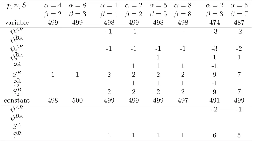
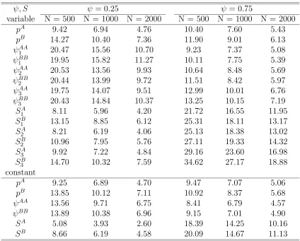
3.5 Converged numbers and Relative biases (%) of estimates of _{p, ψ, S} where either parameters vary over years or those are constant over years with low moving rate (_ψ = 0.25),_pA=_pB= 0_.2_{, S}A= 0_.7_{, S}B = 0_.5_{, N} = 1000. There are three years of tag-recovery and two states. . 73

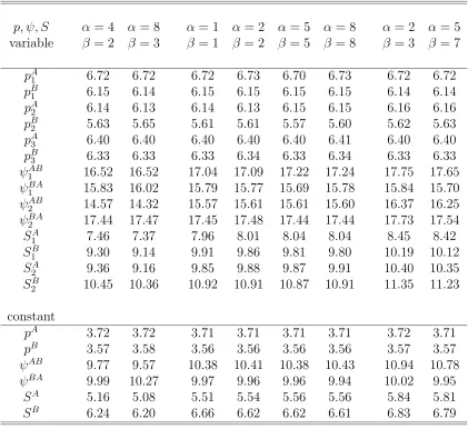
3.6 Converged numbers and Relative biases (%) of estimates of _{p, ψ, S} where either parameters vary over years or those are constant over years with high moving rate (_ψ= 0.75),_pA=_pB= 0_.2_{, S}A= 0_.7_{, S}B = 0_.5_{, N} = 1000. There are three years of tag-recovery and two states. 74 3.7 Relative standard errors (%) of estimates of_{p, ψ, S} where either param-eters vary over years or those are constant over years with low moving rate (_ψ = 0.25),_pA =_pB = 0_.2_{, S}A = 0_.7_{, S}B = 0_.5_{, N} = 1000. There are three years of tag-recovery and two states. . . 75

(11)

3.9 Relative standard errors (%) of estimates of_{p, ψ, S} where either param-eters vary over years or those are constant over years with _pA=_pB = 0_.1_{, S}A = 0_.8_{, S}B = 0_.6. There are three years of capture-recapture and two states. . . 77 3.10 Relative standard errors (%) of estimates of_{p, ψ, S} where either

param-eters vary over years or those are constant over years with _pA=_pB = 0_.2_{, S}A = 0_.7_{, S}B = 0_.5. There are three years of capture-recapture and two states. . . 78 3.11 Relative standard errors (%) of estimates of_{p, ψ, S} where either

param-eters vary over years or those are constant over years with _pA=_pB = 0_.4_{, S}A = 0_.6_{, S}B = 0_.4. There are three years of capture-recapture and two states. . . 79 3.12 Experiment 1. for different amounts of sampling effort on each area . 80 3.13 Experiment 2. for equal sampling effort on each area . . . 80 3.14 The estimates with separation of survival and movement rates . . . . 81 4.1 Tag return array for three years of tagging and recovery with

once-a-year tagging . . . 101 4.2 Multinomial cell probabilities of tag return data for three years of

tag-ging and recovery with once-a-year tagtag-ging . . . 101 4.3 Example not depending on_t. The same natural mortality for each area

over years. The recovery matrix for a once-a-year tagging model for a pulse fishery. There are three tagging and recovery years and two sites or patches. . . 102 4.4 Example with a known movement time, _t = 0_.5. The recovery matrix

for a once-a-year tagging model for a pulse fishery. There are three tagging and recovery years and two sites or patches. . . 102 4.5 Example with a random movement time variable _t, following uniform

distribution. The recovery matrix for a once-a-year tagging model for a pulse fishery. There are three tagging and recovery years and two sites or patches. . . 102 4.6 The estimates for three examples for once-a-year tagging models with

λ = 1_.0. There are three tagging and recovery years and two sites or patches. Fishing mortality rates are estimated for three years and movement rates for two years. Natural mortality rates are assumed constant over years. . . 103 4.7 Example with cell probabilities not depending on_t,which has the same

(12)

4.8 Example with a known movement time, _t = 0_.5. The recovery matrix for a twice-a-year tagging model for a continuous fishery. There are three years of tagging and recovery and two sites or patches. . . 104 4.9 Example with random variable _t, following uniform distribution. The

recovery matrix for a twice-a-year tagging model for a continuous fish-ery. There are three years of tagging and recovery and two sites or patches. . . 105 4.10 The estimates for the three examples for twice-a-year tagging models

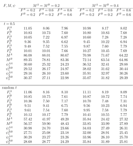
with _λ = 1_.0 and _T = 0_.2. There are three years of tagging and recovery and two sites or patches. Fishing mortality rates are estimated for three years, and movement rates for two years. Natural mortality rates are assumed constant over years. . . 105 4.11 Once-a-year tagging with _M constant over sites (patches), so that cell

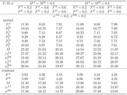
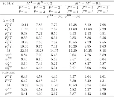
structure does not depend on _t: Relative standard errors (%) of es-timates of _{F, M, ψ} where either parameters vary over years or those are constant over years with _N = 1000 and _λ = 0_.5. There are three tagging and recovery years and two sites or patches. . . 106 4.12 Twice-a-year tagging wit _M constant over sites (patches), so that cell

structure does not depend on _t: Relative standard errors (%) of esti-mates of _{F, M, ψ} where either parameters vary over years or those are constant over years with _N = 1000, _λ = 0_.5, and _T = 0_.1. There are three years of tagging and recovery and two sites or patches. . . 108 4.13 Twice-a-year tagging with _M constant over sites (patches), so that

cell structure does not depend on _t: Relative standard errors (%) of estimates of _{F, M, ψ} where either parameters vary over years or those are constant over years with _N = 1000,_λ = 0_.5, and _T = 0_.2. There are three years of tagging and recovery and two sites or patches. . . . 110 4.14 Once-a-year tagging with _t either fixed or random: Relative standard

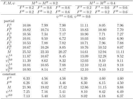
errors (%) of estimates of _{F, M, ψ} where parameters vary over years with _N = 1000, _λ = 0_.5, _ψAA = 0_.2, _ψBB = 0_.2. There are three tagging and recovery years and two sites or patches. . . 112 4.15 Once-a-year tagging with _t either fixed or random: Relative standard

errors (%) of estimates of _{F, M, ψ} where parameters vary over years with _N = 1000, _λ= 0_.5, _ψAA= 0_.6,_ψBB = 0_.6. There are three years of tagging and recovery and two sites or patches. . . 113 4.16 Twice-a-year tagging with_t either fixed or random: Relative standard

(13)

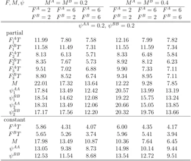
4.17 Twice-a-year tagging with_t either fixed or random: Relative standard errors (%) of estimates of _{F, M, ψ} where parameters vary over years with _N = 1000, _λ = 0_.5, _T = 0_.1 _ψAA = 0_.6, _ψBB = 0_.6. There are three years of tagging and recovery and two sites or patches. . . 115 4.18 Twice-a-year tagging with_t either fixed or random: Relative standard

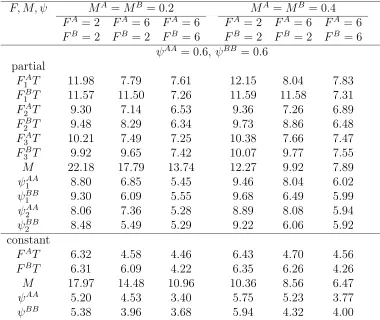
errors (%) of estimates of _{F, M, ψ} where parameters vary over years with _N = 1000, _λ = 0_.5, _T = 0_.2 _ψAA = 0_.2, _ψBB = 0_.2. There are three years of tagging and recovery and two sites or patches. . . 116 4.19 Twice-a-year tagging with_t either fixed or random: Relative standard

errors (%) of estimates of _{F, M, ψ} where parameters vary over years with _N = 1000, _λ = 0_.5, _T = 0_.2 _ψAA = 0_.6, _ψBB = 0_.6. There are three years of tagging and recovery and two sites or patches. . . 117 5.1 Tag return array for two years of tagging and recovery with

twice-a-year tagging . . . 146 5.2 Multinomial cell probabilities of tag return data for two years of tagging

and recovery with twice-a-year tagging . . . 146 5.3 Example of the recovery matrix for a two-site tag-return model for a

pulse fishery with random movement . . . 147 5.4 The mean and standard error for each estimate in four examples for

twice-a-year tagging models with _T = 0_.2 . . . 147 5.5 Example of the recovery matrix for a two-site tag-return model for

a continuous fishery over part of year in the case random movement occurs. . . 147 5.6 Capture histories with associated probabilities for the combined model

of capture-recapture sampling in a marine reserve (A) and tag-return sampling in a fishing area (B) used to generate data for the model . 148 5.7 Example of the recovery matrix for a two-site model with

capture-recapture sampling in a marine reserve and tag-return sampling in a fishing area for a pulse fishery with random movement . . . 149 5.8 Example of the recovery matrix for a two-site model with

capture-recapture sampling in a marine reserve and tag-return sampling in a fishing area for a continuous fishery with random movement . . . 150 5.9 Two-site tag-return model by twice-a-year tagging with random

move-ment: Converged numbers and relative standard errors (%) of esti-mates of _{F, M, ψ} where either parameters vary over years or those are constant over years with _N = 1000,_λA=_λB = 0.5, _ψAA =_ψBB = 0.2. 151 5.10 Two-site tag-return model by twice-a-year tagging with random

(14)

5.11 Two-site tag-return model by twice-a-year tagging with random move-ment: Converged numbers and relative standard errors (%) of esti-mates of _{F, M, ψ} where either parameters vary over years or those are constant over years with _N = 1000,_λA=_λB = 0.5, _ψAA =_ψBB = 0.6. 153 5.12 Two-site tag-return model by twice-a-year tagging with random

move-ment: Converged numbers and relative standard errors (%) of esti-mates of _{F, M, ψ} where either parameters vary over years or those are constant over years with _N = 1000, _λA=0.8, _λB = 0.5, _ψAA =_ψBB = 0.6. . . 154 5.13 Two-site model with capture-recapture sampling in a marine reserve

and tag-return sampling in the fishery area by twice-a-year tagging with random movement: Converged numbers and relative standard errors (%) of estimates of _{F, M, ψ} where either parameters vary over years or those are constant over years with _N = 1000, _λA=_λB = 0.5,

ψAA = _ψBB = 0.2. . . 155 5.14 Two-site model with capture-recapture sampling in a marine reserve

and tag-return sampling in the fishery area by twice-a-year tagging with random movement: Converged numbers and relative standard errors (%) of estimates of _{F, M, ψ} where either parameters vary over years or those are constant over years with _N = 1000, _λA=0.8, _λB = 0.5, _ψAA = _ψBB = 0.2. . . 156 5.15 Two-site model with capture-recapture sampling in a marine reserve

and tag-return sampling in the fishery area by twice-a-year tagging with random movement: Converged numbers and relative standard errors (%) of estimates of _{F, M, ψ} where either parameters vary over years or those are constant over years with _N = 1000, _λA=_λB = 0.5,

ψAA = _ψBB = 0.6. . . 157 5.16 Two-site model with capture-recapture sampling in a marine reserve

and tag-return sampling in the fishery area by twice-a-year tagging with random movement: Converged numbers and relative standard errors (%) of estimates of _{F, M, ψ} where either parameters vary over years or those are constant over years with _N = 1000, _λA=0.8, _λB = 0.5, _ψAA = _ψBB = 0.6. . . 158 5.17 Two-site tag-return model by twice-a-year tagging with random

(15)

5.18 Two-site tag-return model by twice-a-year tagging with random move-ment: Converged numbers and relative standard errors (%) of esti-mates of _{F, M, ψ} where either parameters vary over years or those are constant over years with _N = 1000, _λA=0.8, _λB = 0.5, _ψAA =_ψBB = 0.6, using additional planted tag cohorts with 100 in each patch. . . . 160 5.19 Two-site tag-return model by twice-a-year tagging with random

move-ment: Converged numbers and relative standard errors (%) of esti-mates of _{F, M, ψ} where either parameters vary over years or those are constant over years with _N = 1000, _λA=0.8, _λB = 0.5, _ψAA =_ψBB = 0.6, using an additional planted tag cohort of 500 in patch _A . . . 161 5.20 Two-site tag-return model by twice-a-year tagging with random

move-ment: Converged numbers and relative standard errors (%) of esti-mates of _{F, M, ψ} where either parameters vary over years or those are constant over years with _N = 1000, _λA=0.8, _λB = 0.5, _ψAA =_ψBB = 0.6, using additional planted tag cohorts with 500 in each patch. . . . 162 5.21 Two-site tag-return model by twice-a-year tagging with random

move-ment: Converged numbers and relative standard errors (%) of esti-mates of _{F, M, ψ} where either parameters vary over years or those are constant over years with _N = 1000, a fixed _λA=0.8, _λB = 0.5, _ψAA =

ψBB = 0.6 . . . 163 5.22 Two-site tag-return model by twice-a-year tagging with random

move-ment: Converged numbers and relative standard errors (%) of esti-mates of _{F, M, ψ} where either parameters vary over years or those are constant over years with _N = 1000, fixed _λA=0.8 and _λB = 0.5, _ψAA = _ψBB = 0.6 . . . 164 5.23 Two-site tag-return model by twice-a-year tagging with random

(16)

List of Figures

3.1 Separation of survival and movement rates . . . 82

4.1 Type 1 (pulse) Fishery in once-a-year tagging . . . 118

4.2 Type 2 (continuous) Fishery in once-a-year tagging . . . 119

4.3 Type 2 (continuous) Fishery in twice-a-year tagging . . . 120

(17)

Chapter 1

(18)

In the second chapter the background for this thesis is reviewed using the earlier research literature. In the following three research chapters we present new theory and some applications of how multi-state capture-recapture sampling can be used for tag-return and capture-live recapture experiments to allow estimation of the survival and movement probabilities.

In chapter three we propose the separation of survival and movement rates whereas previous authors have only considered transition probabilities which involve both processes. This topic is very important to conservation biologist interested in meta-population dynamics for endangered or threatened species of wildlife (Nichols et al. 1992). This framework is developed and then used to make simulations for each of tag-return and capture-recapture experiments.

In chapter four we consider special multi-state models applicable to modern fish-eries tag recovery studies. We build on models developed by Brownie et al. (1985), Pollock et al. (1991, 1995), Hoenig et al. (1998 a, b), and Hearn et al. (1998) on twice-a-year tagging for single state models. We also use some of the results on separation of survival and movement rates developed in chapter three. We consider models for both once-a-year tagging and twice-a-year tagging.

(19)

Chapter 2

(20)

2.1 Traditional Capture-Recapture Models

2.1.1 The Lincoln-Petersen Model

This simplest form of capture-recapture method has a long history going back to Laplace in 1786, who used it to estimate the human population size of France (Seber 1982 _p.104). The first uses of the two sample mark-recapture method, in animal population ecology, was by Petersen around the turn of the century (Le Cren 1965) for fisheries, and later was used by Lincoln (1930) for wildlife studies.

A sample of _n₁ animals is caught, marked, and released. Later a sample of _n₂ animals is captured, of which _m₂ have been marked. Intuitively one can derive an estimator of the population size (_N) based on the notion that the ratio of marked to total animals in the second sample should reflect the same ratio in the population so that

m2

n2 ≈

n1

N,

which gives the estimator

ˆ

N = n1n2

m2 .

A modified version with less bias was originally given by Chapman (1951) as

ˆ

Nc = (n1+ 1)(n2+ 1) (_m₂+ 1) −1

with an approximately unbiased estimate of its variance given by

ˆ

var( ˆ_N_c) = (n1+ 1)(n2 + 1)(n1−m2)(n2−m2) (_m₂+ 1)2(_m₂+ 2)

(21)

All capture-recapture studies are based on models with important model assump-tions which may or may not be satisfied in real populaassump-tions. In the Lincoln-Petersen model, the assumptions are:

1. The population is closed to additions (births or immigrants) and deletions (deaths or emigrants).

2. All animals are equally likely to be captured in each sample. 3. Marks are not lost and are not overlooked by the observer.

The second assumption, which is often called the assumption of “equal catchabil-ity” of animal, in particular, is unlikely to be true in many wild populations. It is important to distinguish two very different types of alternatives.

1. Heterogeneity - The probability of capture in any sample, is a property of the animal and may vary over all the animals in the population. This variation in capture probability could be due to many factors such as age, sex, social status, or “territory” location in relation to trap position.

2. Trap response - The probability of capture in any sample depends on the animal’s prior history of capture i.e., marked animals may have a lower (trap-shy) or a higher (trap-happy) capture probability than unmarked animals.

2.1.2 Closed Population Models

(22)

fully developed by Otis et al. (1978).

The models differ in the manner in which capture probability is modeled. Different models consider combinations of three sources of variation in capture probability: (1) heterogeneity, (2) trap response, and (3) temporal variation or variation among sampling periods (e.g., capture probability for day _i differs from that for day _j). A computer program called CAPTURE contains a model selection procedure that aids the biologist in choosing the most appropriate model for a particular data set.

M0: The Equal Catchability Model

This model assumes that every animal in the population has the sample probability of capture (_p) for each sampling period in the entire study. It is mainly included for pedagogic reasons and to provide a basis for generalization.

It should be emphasized that this estimator can be highly biased if there is unequal catchability of any kind.

Mh: The Heterogeneity Model

(23)

that sometimes works well. Unfortunately, however, it may not be feasible in small populations.

Mb: The Trap Response Model

Model _M_b allows trap response but no heterogeneity or temporal variation and makes the following assumptions:

1. Every unmarked animal in the population has the same probability of capture (_p) for all samples.

2. Every marked animal in the population has the same probability of recapture (_c) for all samples after it has been captured once.

Animals do not contribute any information for population size estimation after first capture. Thus this model is equivalent to the “removal” method (Zippin 1956; Seber 1982 _p.309), except in this case an animal is not physically removed but is considered removed after initial marking.

Often a linear regression method has been used to estimate_N, however, we believe use of the MLE in program CAPTURE is better. We have found that there is usually little difference between the two estimators.

Mbh: The Heterogeneity and Trap Response Model

(24)

Chao (1991), Norris and Pollock (1996) and Pledger (2000) have proposed promising nonparametric approaches to derive estimators of population size for this model.

Mt: The Schnabel Model (Time Variation)

Model _M_t does not allow heterogeneity or trap response of the individual animal capture probabilities. It has a history going back to Schnabel (1938). The model assumes that every animal in the population has the same probability of capture at each sampling time,_p_i;_i= 1_,2_{, ..., k}.

I strongly recommend the use of program CAPTURE because it provides an MLE. Unlike the other models this model does not require detailed capture history infor-mation. Batch marks are sufficient to allow estiinfor-mation.

Other Time Dependent Models

The three important models _M_h, _M_b, and _M_bh all require the assumption that capture probabilities do not vary over time.

We now consider unequal catchability models which do allow time variation.

Mth: The Time Variation and Heterogeneity Model

This model implies that variation in capture probability, due to time and hetero-geneity, is independent. The model does not allow for trap response. An estimator is provided by Chao et al. (1992).

Mtb: The Time Variation and Trap Response Model

Model_M_tb assumes that the capture probability of an animal changes after initial capture. The model also assumes that environmental conditions over time affect the capture probabilities. Lloyd (1994) developed a martingale estimator for this model and studied the efficiency compared to that of the _M_t model.

(25)

Model _M_tbh allows for time variation, heterogeneity, and trap response. No esti-mator is currently available for this model.

Model Selection

It is difficult to select a model from the set but program CAPTURE does include such a procedure. Menkins and Anderson (1988) recommend the use of the Lincoln-Peterson estimate, based on pooling of samples, which is preferable to use of program CAPTURE, if populations are small and/or if the capture probability is very low. Pledger (2000) has developed a model selection procedure based on AIC for the finite mixture approach.

2.1.3 Open Population Models

In many capture-recapture studies it is not possible to assume that the population is closed to additions and permanent deletions.

The Jolly-Seber Model

The basic open population model suitable for this situation is the Jolly-Seber model (Jolly 1965; Seber 1965). The Jolly-Seber model allows estimation of popula-tion size at each sampling time as well as survival rates and birth numbers between sampling times. It also allows estimation of capture probabilities.

Assumptions and Notation

1. Every animal present in the population at the time of the _ith sample (_i = 1_,2_{, ..., k}) has the same probability of capture (_p_i).

(26)

3. Marks are not lost or overlooked.

4. All samples are instantaneous and each release is made immediately after the sample.

Assumptions (1), (3), and (4) were required under the Lincoln-Peterson model. Because only marked animals are used to estimate survival rates, we do not need to assume that marked and unmarked animals have equal survival rates. However, in practice, biologists will want to use the survival estimates to refer to the whole population rather than just the marked component. The Jolly-Seber model allows for “losses on capture” i.e., some animals may not be returned to the population after capture. Implicit from the above assumptions is that all emigration from the popu-lation is permanent. We also emphasize that it is not possible to separate permanent emigration from mortality so that our _p_i parameters are 1 - mortality - emigration, and only represent true survival if permanent emigration is negligible.

Parameters

Mi = the number of marked animals in the population at the time theith sample is taken (_i= 1_{, ...k};_M_i = 0).

Ni = the total number of animals in the population at the time theith sample is taken (_i= 1_{, ...k}).

Bi = the total number of new animals entering the population between the ith and (_i+ 1)th sample (_i= 1_{, ...k}−1).

φi = the survival probability for all animals between theith and (i+ 1)th sample (_i= 1_{, ..., k}−1).

pi = the capture probability for all animals in theith sample (i= 1, ..., k−1).

(27)

mi = the number of marked animals captured in the ith sample (i= 1, ..., k).

ui = the number of unmarked animals captured in the ith sample (i= 1, ..., k).

ni =mi+ui, the total number of animals captured in theith sample (i= 1, ..., k).

Ri = the number of ni that are released after the ith sample (i = 1, ..., k −1). This may not be all of the_n_i due to losses on capture.

ri = the number of the Ri animals released at i that are captured again (i = 1_{, ..., k}−1).

zi = the number of animals captured before i, not captured at i, and captured again later (_i= 2_{, ..., k}−1).

The statistics required for calculation are summary statistics from the complete capture-history information for each animal captured at least once in the study.

Explicit estimates are available for the full Jolly-Seber model, but constrained models require iterative solutions. Cormack (1973) gave a brief intuitive description of this model and its estimators, and Seber (1982 _p.196) gave the best detailed pre-sentation. Comprehensive computer programs are available to help with analyses under this model (e.g., POPAN-3, Arnason and Schwarz 1987; SURGE, Lebreton et al. 1992; JOLLY, Pollock et al. 1990; MARK, White and Burnham 1999).

Influence of Assumption Violations

(28)

any sample (_m_i_/n_i) will tend to over-estimate the true proportion of marked animals in the population (_M_i_/m_i). This leads to a negative bias in ˆ_N_i. In addition, Pollock et al. (1985) have noted that the estimator ˆ_M_i is derived intuitively by equating the proportions of two groups of marked animals in the population just after period _i (those seen at_{i, R}_i; and those not seen at_i, _M_i−_m_i) that are captured at some sub-sequent period (_{> i}). Heterogeneity can result in a somewhat larger average capture probability for those animals caught at_i (_R_i) than marked animals not caught then (_M_i −_m_i). This results in a relatively small negative bias in ˆ_M_i (Carothers 1973). Biased_M_i contribute not only to the bias of ˆ_N_i, but also result in biased ˆ_φ_i, but this bias is usually small.

(29)

is negatively biased if the animals are trap-happy, and positively biased if the animals are trap-shy.

If marking decreases the animal’s survival rate, serious negative bias can occur in the survival rate estimators. However, there is no bias in population size estimates.

The assumption of no tag loss is also very important, because if animals lose their marks the number of recaptures will be too low and there is serious bias in survival estimates but no bias in population size estimates.

Another implied assumption is that any emigration from the study area is perma-nent. Temporary emigration is likely to occur in some practical field situations, and the bias induced could be serious (Pollock et al. 1985).

2.2 Other Open Models

2.2.1 Survival Modeling

(30)

estimation problem. The likelihoods they consider are conditional on first capture and are the products of multinomial distributions. Estimation is straight forward using maximum likelihood methods.

Lebreton et al. (1992) emphasize that their paper synthesizes, using a common framework, recent developments together with new ones, with an emphasis on flexibil-ity in modeling, model selection, and the analysis of multiple data sets. The effect on survival and capture rates of: time, age, and categorical variables characterizing the individuals (e.g., sex), can be considered, as well as interactions between such effects. This “analysis of variance” philosophy emphasizes the structure of the survival and capture processes rather than the technical characteristics of any particular model. The flexible array of models encompassed in this synthesis uses a common notation. As a result of the greater level of flexibility and relevance that is achieved, the focus is changed from fitting a particular model to model building and model selection.

2.2.2 Comparative Capture-Recapture Studies

Burnham et al.(1987) present design and analysis methods for comparative sur-vival experiments based on release-capture of marked populations. The methods pre-sented apply to any experiments involving treatment and control groups of marked animals. A primary application was to address fishery survival issues on the Columbia River in the Northwest of the USA. Treatments involved fish passing through hydro-electric turbines, and controls involved fish that were added below the turbines on the river. Testing for differences between treatment and control groups was a primary focus.

(31)

which is based on program SURVIV (White 1983) was developed by Gary White (Burnham et al. 1987) to handle this type of comparative design.

2.2.3 The Robust Design

Introduction

At the basis of many capture-recapture sampling models is the assumption that all animals are equally likely to be caught in each sample (the equal catchability assumption). This assumption is most unlikely to be realistic in natural animal pop-ulations, and either one or both of the heterogeneity and trap-response alternatives may be acting in a particular animal population.

The capture-recapture model most frequently used by biologists for open popu-lations in long-term studies is the Jolly-Seber model. This model requires the equal catchability assumption and although some weakening of the assumption is possible, the complexity of open population models is likely to preclude general models that allow heterogeneity and/or permanent trap response. However, some closed models do permit relaxation of the equal catchability assumption in a biologically realistic manner.

(32)

population size estimation under models allowing unequal catchability while survival estimation, which is not so affected by unequal catchability, is under the Jolly-Seber Model.”

Pollock (1982) noted some limitations of the Jolly-Seber model and proposed the “robust design”, a sampling scheme that combines the features of both closed and open population model analyses.

The Basic Design

We consider the following representation of a capture-recapture sampling experi-ment.

Primary

Periods 1 2 · · · _k

Secondary

Periods 1 2 · · · _l₁ 1 2 · · · _l₂ · · · 1 2 · · · _l_k

We have _k primary sampling periods (e.g., months or years depending on the species), and within each one of these we have _l_i(_i = 1_{, ..., k}) secondary sampling periods that are very close to each other in time (e.g.,_l_iconsecutive days of trapping). It is not necessary that the number of secondary periods be equal in all the primary periods but it usually is.

The design can be used to estimate the population size for each of the pri-mary periods (_N₁_{, N}₂_{, ..., N}_k), assuming that the population is constant over the sec-ondary sampling periods within each primary sampling period. One also can estimate survival rates (_φ₁_{, φ}₂_{, ..., φ}_k−₁) between the primary sampling periods and numbers of new individuals entering the population between the primary sampling periods (_B₁_{, B}₂_{, ..., B}_k−₁)

(33)

Bk−1using the standard Jolly-Seber model. In order to use the Jolly-Seber model with

the described design, all the secondary sampling periods within a primary sampling period would be “pooled”. Here by “pooled” we mean that we are just interested in whether or not an animal is captured at least once during the primary sampling period.

When considering the use of the Jolly-Seber model, it is important to keep in mind the requisite assumptions and model robustness. It was pointed out that heterogene-ity and/or trap response will have a large effect on the population size estimators because the sample ratio (_m_i_/N_i) will no longer accurately reflect the population ra-tio (_M_i_/N_i). The marked population estimators will not be so affected by unequal catchability because the two ratios of recoveries of marked animals will both tend to be influenced similarly. It follows that the survival rate estimators, which are simply ratios of the ˆ_N_i’s, also will be less affected by unequal catchability than the popu-lation size estimators. Cormack (1972) suggested this using an intuitive argument and Carothers (1973) documented it for heterogeneity of capture probabilities using analytic approximations and computer simulation. In the case of permanent trap response, survival rate estimates are not affected at all (Nichols et al. 1984).

In the robust design we attempt to minimize the influence of unequal catchability on our estimators by exploiting our two levels of sampling. Survival rate estimators, which are not so influenced by unequal catchability, will be estimated exactly as under the Jolly-Seber procedure using pooled captures within a primary periods. These survival estimators will be available only for _i= 1_,2_{, ..., k}−2.

(34)

estimates use only the captures and recaptures within a primary sampling period. The easiest way for a biologist to obtain these captures is to use the program CAP-TURE developed by Otis et al. (1978) (also White et al. 1982). This program considers a range of different models allowing for heterogeneity and/or trap response and also gives an objective method of choosing the most appropriate model to use. An additional advantage of this approach is that population size estimators are avail-able for all primary periods (_i = 1_{, ..., k}), whereas under the Jolly-Seber approach, estimators are only available for_i= 2_{, .., k}−1. Caution is suggested in the use of the model selection procedure from CAPTURE (Chapman 1980; Menkins and Anderson 1988). The tests are not independent and often have low power, especially for small populations (Menkins and Anderson 1988).

Finally, birth rates can be estimated, but now the population size estimators used are those described in the preceding paragraph. It is possible to estimate_B₁_{, ..., B}_k−₂, whereas under Jolly-Seber it is only possible to estimate _B₂_{, ..., B}_k−₂. If one had an estimator of _φ_k−₁ then _B_k−₁ would also be estimable. In some experiments, it may be reasonable to estimate_φ_k−₁ by _φ_k−₂ or perhaps by an average of ˆ_φ₁_{, ...,}_φˆ_k−₂. Advantages

Here I very briefly list and discuss the important advantages of the design (Pollock et al. 1993).

(35)

2. All parameters can be estimated. Under the Jolly-Seber model not all param-eters are estimable. For example, _N₁_{, N}_k_{, φ}_k−₁_{, B}₁, and _B_k−₁ in a _k primary period study are not estimable whereas, under the robust design, all these parameters are estimable. Notice that some parameters can be estimated in more than one way.

3. Alternative estimators are available for most parameters. Discrepancies be-tween these alternative estimators might be useful in assessing assumption violations. 4. Abundance and Survival can be estimable for most parameters. Under den-sity dependent population models the focus of attention for ecologists is the true function relationship between abundance (density) and survival. If the Jolly-Seber method provides estimators for abundance and survival, the true functional relation-ship between density and survival will be confounded with the statistical dependence between their estimators. Kendall (1992) found, using simulation, that there is a very weak relationship between population size and survival when the ad hoc estimation procedure of the robust design is used. Thus the true functional relationship between density and survival is less likely to be obscured when the robust design estimators are used.

(36)

effort.

6. Practical advantages over the Jolly-Seber design (i.e., only one secondary period per primary period) exist. For example, under the robust design, a biologist might sample intensively for four consecutive days and then take three weeks off before repeating the process. Alternatively, a biologist may sample one day each week of the month and use the Jolly-Seber estimators. It seems that resources are much better utilized under the robust design scenario. For the other three weeks, the biologist might carry out other studies (habitat analyses etc. ).

7. There is the possibility of separation of in-situ reproductive recruitment and immigration in a two age class model (Nichols and Pollock 1990).

William Kendall, (Kendall and Pollock 1992; Kendall et al. 1995) has studied the robust design in great detail. He considered ML estimation when heterogeneity was not present. He carried out some comprehensive simulation studies which showed the value of the robust design over regular open models like the Jolly-Seber model.

(37)

2.3 Tag-Return Models (Band Recovery Models)

2.3.1 The Brownie Models

Many researchers focus considerable attention on the estimation of survival rates and specifically concentrate on inference procedures (estimation and hypothesis tests) regarding time- and age-specific survival rates (see in particular Brownie et al. 1985). They examine animal banding or tagging studies where: (1) A number of animals are caught and banded (tag, mark) each time period (year, month, week) for_k such equal time periods (often the time period is a year). Generally each band or tag carries a unique number or code. (2) Records are kept of bands or tags reported from dead animals (often obtained from hunting or fishing) for each time period from each batch banded. Therefore the recovery data conveniently form an array representing the number of bands or tags recovered in time period_j from those animals originally banded in time period_i.

Notations and Definitions

For _k banding occasions let _N₁_{, ..., N}_k be the numbers banded and released back into the population. Equal time intervals between banding is typically assumed. Let the band recovery data be represented by _R_ij defined as _R_ij = the number of band recoveries in hunting season_j from birds originally banded in year_i. The method for displaying data is shown on Table 2.1 in this symbolic notation.

(38)

For adults of one species and sex, there will be just one such recovery data array per study. Often, however, both young and adults are banded from the same species and population. Then there will be two such data arrays to consider for statistical analysis. For wildlife species less often, three age classes are banded: young, subadults, and adults. However, for fish species there will often be many age classes.

Parameters

S = an annual survival rate; the probability that an animal, alive when a given cohort is banded, will survive one calendar year, to the time of next banding.

f = an annual band recovery rate; the probability that a banded animal, alive when a given cohort is banded, will be harvested and its band reported during the next hunting season.

f = _λH

where_λ= banding reporting rate = probability that a hunter or fisher will report the band, given that he has killed and retrieved a banded animal

H = harvest rate or probability of being killed and retrieved by hunter or fisher during the year

H =_cK where _crepresents a retrieval rate

K = kill rate

(39)

the hypothesis concerning how _S and _f vary.

Consider the hypothesis (tentative assumption) that survival, hunting, and re-porting rates are constant over age, but vary by year (Model 1 in Brownie et al. 1985). This model is characterized as in Table 2.2 in terms of the expected or average numbers of band recoveries, expressed as functions of _N_i, _f_i, and _S_i with _k = 3, _l = 4.

The expectations, under the assumptions that recovery and survival rates are time-specific, can be expressed in terms of parameters as:

E(_R_ii) = _N_i_f_i_{, i}= 1_{, ..., k}

E(_R_ij) =_N_i_S_i_...S_j−₁_f_j_{, i}= 1_{, ..., k, j} =_i+ 1_{, ..., l}

The survival/migration parameters_S₁_{, ..., S}_k−₁and recovery rate parameters_f₁,...,_f_k are estimable whether _l = _k or not. If, however, _{l > k} the parameters _S_k,...,_S_l and_f_k₊₁,...,_f_l are separately estimable; only confounded parameters representing the products of survival and recovery in years_k+1_{, ..., l}such as_S_k_f_k₊₁,_S_k_S_k₊₁_f_k₊₂,...,_S_k..._S_l−₁_f_l are estimable.

Assumptions

(1) The sample is representative of the target population; (2) age and sex of individuals are correctly determined; (3) there is no band loss;

(4) survival rates are not affected by the banding or tagging itself;

(40)

individuals;

(7) all banded individuals of an identifiable class (e.g., by species, age, sex) in the sample have the same annual survival and recovery rates.

We note that annual survival and recovery rates may vary by calendar year, and/or by age and sex of individuals (variation of survival and recovery rates by area (pop-ulation) is also possible). Also as part of the analysis of recovery data, under any given model, a goodness of fit test is usually given to judge whether the model is an acceptable fit to the data. These goodness of fit tests are meant to be used in the processes of selecting the appropriate model for any given data set. Model selection also often uses likelihood ratio tests and the Akaike Information Criteria (AIC).

2.3.2 Fisheries Tag Return Models

The primary purpose of the Brownie models (Brownie et al. 1985) was to estimate the annual survival rates (_S). Recently, fisheries biometricians have extended these models to the estimation of fishing and natural mortality. They also use a slightly different notation involving instantaneous rates (Ricker 1975; Pollock et al. 1991, 1995; Hoenig et al. 1998a, 1998b).

Model definition

S = the finite survival rate or the probability of surviving the year;

u = _H = finite annual exploitation rate or the probability of being harvested (Ricker’s rate of exploitation);

λ = tag reporting rate, or the probability that a tag will be found and reported to the fisheries biologist, given that the fish has been harvested;

(41)

Model Assumptions

Fisheries biologists usually use an instantaneous rates formulation which makes an additional assumption that fishing and natural mortality rates are additive. We define:

Fi = the instantaneous rate of fishing mortality in year i;

Mi = the instantaneous rate of natural mortality in year i. The finite annual survival rate in year _i is: _S_i =_exp(−(_F_i+_M_i)) We usually assume _M_i is constant over years for a particular age class.

The finite annual exploitation rate (_u_i) has different forms for different types of fisheries (Ricker 1975): for Type 1 (pulse) _u_i = 1−_exp(−_F_i); and for Type 2 (continuous)_u_i = Fi

Fi+M{1−exp(−(Fi+M))}.

Hoenig et al. (1998 a) gave more general forms for other patterns of fishing. The separate estimation of _F_i and _M depends on having an estimate of report-ing rate (_λ). There are a variety of methods of estimating reporting rates which include reward tagging of observers, angler/port surveys, and planting tags in the catch (Pollock et al. 2000). One special method of estimating reporting rate is to use twice-a-year tagging (Hearn et al. 1998).

(42)

2.4 Stage-Structured Capture-Recapture Models

2.4.1 Population Projection Models

The Leslie Matrix approach to population analysis (Bernardelli 1941; Lewis 1942; Leslie 1945, 1948) has seen wide use in animal population ecology. In this approach, the population size at time _t is characterized by a column vector, n_t, containing the number of animals in each age class. The population at time _t+ 1 is then projected using a matrix,L, of age-specific survival and fecundity rates:

Ln_t =n_t₊₁

During the last 15 years many ecologists have realized that vital rates may be closely associated with characteristics of organisms other than age (e.g., Werner and Caswell 1977; Hughes 1984; Sauer and Slade 1987; Caswell 1989). This realization has led to the increased use of stage-based matrix models, which are similar to the age-structured models, except thatn_t contains the number of animals in each stage at time_t, andL is a matrix of stage-specific fecundities and stage-transition probabilities. There has been much work done on the analysis and asymptotic behavior of such models once a projection matrix has been specified ( reviewed by Caswell 1989), but little effort has been expended on methods for estimating the component elements of the projection matrix.

(43)

et al. 1985; Clobert et al. 1987; Pollock et al. 1990; Lebreton et al. 1992) permit estimation of age-specific survival rates, and these estimates can be used directly in age-based population projection models (Leslie 1945; Caswell 1989). A limitation of the Jolly-Seber and other traditional methods, however, is that the tag-recapture or tag-recovery data do not allow for a stochastic transition between stages. Stages that may have stochastic transition probabilities include geographic location and size or weight classifications. Stage membership for a given period is unknown if the animal is not captured. Multi-state models for capture-recapture data were first considered a long time ago by Chapman and Junge (1956); Darroch (1961); and Arnason (1972, 1973). Arnason provides estimators of the transition probabilities between stages which are inefficient if the number of capture periods is greater than 3. There was then a long period where they were neglected. Recently there has been a resurgence of interest in these models. Schwartz et al. (1993) describe a FORTRAN program for calculating the maximum likelihood estimates of transition probabilities for Arna-son’s model. These probabilities constitute the entries of a transition matrix model, and this approach has been called the Arnason- Schwarz Model.

We now review these multi-state capture-recapture and tag-return models in detail because they form the basis of the chapters which follow.

2.4.2 Multi-state Capture-Recapture and Tag-Return

Mod-els

The Arnason-Schwarz Model

(44)

the standard Jolly-Seber study. Thus a marked animal may be recaptured (resighted) more than once, and the complete capture history for each animal includes not only the time of each capture but also the stratum in which capture occurs.

Assumptions and Notations

1. Transition between states depends only on the state at the current time_i(i.e., Markovian transition probabilities).

2. Capture and transition probabilities are the same for all animals in a state at a given period. (This is analogous to the homogeneous capture and survival assumption in the Jolly-Seber and Brownie models.)

3. There is no tag loss.

4. Animals behave independently with respect to capture and transition proba-bilities.

5. Losses to the population from emigration are permanent.

Statistics

nri = the number of animals caught in class (stage) r at timet (t = 1,2, ..., k)

Rr_i = the number marked (new) animals released in sample period _i in class_r

mrs_ij = the number of marked animals caught in period _j in class _s that were previously caught in period _i in class_r

Parameters

φrs_i = the probability of being alive and in stratum_s at time_i+ 1, for an animal alive and in stratum _r at_i;

ps_i = the probability of capture at _i for a animal on stratum_s at _i.

(45)

of the transition and capture probabilities can be estimated for time _i = _k−1, but each parameter cannot be estimated separately (Nichols et al. 1992). The parameters can be separated for _i= 1_,2_{, ..., k}−2.

For simplicity, assume that _a= 3 strata with _k = 4 capture occasions. The basic Jolly-Seber parameters and data are now matrices with rows and columns indexing strata. In addition, matrix elements have subscripts that denotes strata and sub-scripts that denote time or capture occasion. The transition matrix between each time period is:

Φ_i =

     

φ11_i φ12_i φ13_i φ21_i φ22_i φ23_i φ31_i φ32_i φ33_i

    

, i= 1,2,3

Note thatΦ_i is similar to the projection matrix. The differences are thatΦ_idoes not include fecundities and can vary with time.

The release-recapture data are represented in detail in Table 2.3, where each row represents the distribution of the first recaptures of the_Rr_i animals released in a given year _iand stratum _r.

If the assumptions of the model are met, the recapture data follow a product of multinomial distributions. This allows for the estimation of model parameters using maximum likelihood. Program MSSURVIV is designed for this purpose and uses the recapture matrices as input (Brownie et al. 1993). Goodness of fit tests, to determine how well a model describes the data, can then be utilized by comparing expected capture histories with actual capture histories.

(46)

Nichols et al. (1992) describes and application of using capture-recapture data and the multi-state modeling approach in a study of a population of meadow voles (Microtus pennsylvanicus) at Patuxent Wildlife Research Center, Laurel, Maryland during 1981-1982. They estimated survival and transitions between mass classes. In this study, the primary periods of interest were roughly one month apart. Each primary period 1 involved five secondary periods (days) of trapping from 3 to 7 October 1981, period 2 was from 31 October to 4 November 1981, and period 3 was from 4 to 8 December 1981. The goal of the study was to estimate transition probabilities between periods 1 and 2, and periods 2 and 3. However, the multi-state model estimation approach required an additional sampling period. This was necessary in order to obtain an estimate of the number of marked animals at period 3 (Pollock et al. 1990). For this estimate, Nichols et al. (1992) defined the following random variable to be used in conjunction with the previously defined Arnason-Schwarz statistics and parameters, developing the multi-state modeling approach.

Mirs = the number of marked animals alive and in classs in sample period ithat were caught in class _r in period _i−1

The study design included a 10× 10 live-trapping grid with traps stations placed 7.6-m intervals, and baited with whole corn. At each capture of the first three primary periods, voles were assigned to one of four mass classes: A,_<22g (defined as juveniles by Krebs et al. 1969); B, 22-33g (subadults of Krebs et al. 1969); C, 34-45g; D,_>45g. Mass class was assigned based on mass at first capture within a primary period. Sexes were combined in order to obtain good sample sizes for the analysis.

(47)

the study and thus were assumed to be zero. Nichols et al. (1992) parameterized two different multi-state models: general model (denoted Model 1) with_φrs₁ and _φrs₂ ; and reduced parameter model (denoted Model 2) in which specific transition probabilities for periods 1 and 2 were constrained to be equal (_φrs₁ =_φrs₂ =_φrs).

Model 1 provided estimates for each of the estimable time periods, 1 and 2, whereas Model 2 provided a single estimate for each transition probability under the hypoth-esis of no temporal variation. The point estimates for periods 1 and 2 under Model 1 differ substantially in some cases (e.g., BB and DC). The goodness of fit test statis-tic for Model 1 indicated marginal fit, whereas the statisstatis-tics for Model 2 indicated rejection of the models for this data set. A likelihood ratio test between models 2 and 1 also provided evidence that time-specific transition parameters of Model 1 were needed to model these data adequately. In other words, transition probabilities varied significantly between time periods. This variation may need to be taken into consideration in order to model the population dynamics accurately.

Hestbeck et al. (1991) describe an application of using mark-resight data on Canada geese to estimate transitions for Canada geese (Branta canadensis) between geographic areas in the Atlantic flyway. The Atlantic flyway was divided into three strata: the mid-Atlantic (New York, Pennsylvania, New Jersey), Chesapeake (Delaware, Maryland, Virginia), and the Carolinas (North and South Carolina). Mark-resight data from 28 849 Canada geese banded with individually coded neck bands were used to estimate the probabilities of returning to previous wintering locations and moving to new locations.

(48)

and future reproductive “benefits” of returning to the same wintering area include: a familiarity with the distribution of food resources, roost sites, cover, and predators (Raveling 1969; Spaans 1977; Nichols et al. 1983). However, if the relative suitability of different wintering sites, with respect to factors affecting fitness, varies from year to year, and if this variation can be perceived by the birds, then opportunistic selection of the “most suitable” wintering grounds could occur each year (Nichols et al. 1983). In this study, two separate models were used to describe movement and site fidelity. The first model (MV1) assumes a first-order Markov chain, so that the predicted wintering ground location in year _i+ 1 depends only on wintering location in year _i. The second model (MV2) assumes a second-order Markov chain so that the predicted wintering ground location in year _i+ 1 depends on wintering locations in years _i and _i−1. The estimates from the models are used to evaluate hypotheses about wintering site fidelity, directionality of changes in wintering sites, and the possible effects of weather on shifts.

Adult and subadult Canada Geese, with uniquely coded yellow neck bands were resighted during the fall and winter of 1983-1984, 1984-1985, and 1985-1986 in the mid-Atlantic, Chesapeake, and Carolinas. Observers traveled specific routes within the eight states and recorded 101 732 resightings. Each state was surveyed every 1 to 3 weeks from October to April, 1983 through 1988.

The sampling period used to estimate movement rates was defined as 4 January to 15 February. This period excludes the fall migration and corresponds to the time when most geese are at their southern terminus.

(49)

Chesapeake, and C for the Carolinas. They also use 0 to denote the event that an individual was not observed during a given sample period. For example, history A0B denotes a goose captured or observed in region A during year_i, not seen during year

i+ 1, and observed in region B during year_i+ 2.

In the Arnason-Schwarz Model, it is assumed that birds behave independently with respect to sighting probability, survival, and movement. This assumption will be violated for geese because geese do not behave as independent entities (Sulzbach and Cooke 1978). Although this will not bias any estimators, the true sampling variances are larger than those computed from the statistical models for the data (see also Pollock and Raveling 1982).

The assumption that sampling is instantaneous can never be strictly met. Be-cause all mortality for the Arnason-Schwarz Model and all movement and mortality for model MV1 should occur between samples, estimation of survival or transition probabilities is sensitive to the length of the sampling and intersampling periods. Thus, the length of the sampling period should be small compared to the length of time between sampling, and sampling should not occur during periods of high mor-tality, such as times of migration. As noted earlier, sampling for this experiment occurred 3 months after the opening of the hunting season in the northern states, during the time when geese are more sedentary, and at their southernmost terminus. The assumptions for model MV2 are similar to those for model MV1 except that the second assumption in Arnason-Schwarz Model is modified to allow that all marked birds with the_φ0rs_i₊₁or_φ∗rs_i₊₁transition probabilities have the same probability of moving from region_rto_s, given that the bird was either inside or outside of region_s at time