A Space-Frequency Anti-Jamming Algorithm Based on Sub-Band
Energy Detection
Ruiyan Du1, 2, Jiaqi Yang1, 2, *, Lei Liu1, 2, Fulai Liu1, 2, and Hui Song1, 2
Abstract—For most of space-frequency joint anti-jamming algorithms, the solution of adaptive steering vector is a high complexity problem. To solve this issue, a space-frequency combined anti-jamming algorithm based on sub-band energy detection (SF-SED) is proposed. At first, the algorithm performs fast Fourier transform (FFT) on the received data of the array antenna and obtains multi-snapshot data of each sub-band through sub-band decomposition. Then, the interference detection statistic and decision threshold are constructed by the energy of the sub-band to judge whether there is an interference in each sub-band. Finally, different methods are used to solve the adaptive weights of the two types of sub-bands according to sub-band classification results. Compared with the related work, the proposed algorithm not only has lower computational complexity, but also has higher output signal-to-interference-and-noise ratio. Theoretical analysis and simulation results demonstrate the anti-jamming performance of the proposed method.
1. INTRODUCTION
With the increasingly fierce military confrontation, the potential security threat to satellite navigation becomes an intractable problem [1]. Currently, the major anti-jamming researches of global navigation satellite system (GNSS) mostly focus on receivers [2, 3]. Receiver antennas have a great influence on the anti-jamming performance of GNSS. In part of the researches on uniform linear array, [4] puts forward an effective and low-complexity linear arrays synthesis method which still has good performance when an even distribution is required on element excitations. Besides, the researches on anti-interference algorithms are also significant. Most anti-interference algorithms use adaptive filtering technology to process the received signals in the digital domain, e.g., time-domain filtering, frequency-domain filter, spatial filtering, space-time adaptive filtering, space-frequency adaptive filtering, and multi-beam technology [5, 6]. Compared with time and frequency domain filtering, spatial filtering has lager anti-jamming degree of freedom (DOF) and can suppress more kinds of interferences, including broadband interferences. However, when interference signals and satellite signals have the same frequency or direction of arrival (DOA), it is difficult for single-dimensional filtering technology to achieve ideal anti-jamming effect.
Space-time adaptive processing (STAP), which was first proposed by Frost, III in 1972, adds delay taps behind each antenna on the basis of spatial filtering [7]. STAP combines the received data of spatial domain and time domain as the input signals, which not only increases DOF but also has the ability to suppress multipath and wideband interferences. In 2000, the application of STAP in global position system (GPS) was discussed by Fante and Vacarro [8], which is one of the most important techniques in GPS anti-interference at present. For the past few years, quite a few excellent STAP algorithms have been proposed to improve performance from different perspectives [9–11]. In [9] and [10], the
Received 16 May 2019, Accepted 8 July 2019, Scheduled 22 July 2019 * Corresponding author: Jiaqi Yang ([email protected]).
1 Engineer Optimization & Smart Antenna Institute, Northeastern University at Qinhuangdao, Qinhuangdao, China. 2 School of
robustness of STAP algorithm is improved by reconstructing signal covariance in different ways. A proportion differentiation algorithm is proposed to control time taps so that the interferences can be suppressed more effectively [11].
However, it is known that the STAP algorithm has a large amount of computation due to calculating the inverse of the covariance matrix, so that the low-complexity sub-optimal solution space-frequency adaptive processing (SFAP) algorithm has been extensively studied as well [12]. The core idea of the SFAP algorithm is to convert received GPS signals into the frequency domain by fast Fourier transform (FFT) so as to perform sub-band decomposition, then the adaptive weights are calculated on each sub-band, respectively, thereby the dimensionality reduction processing of the covariance matrix is realized [13]. Some achievements have been made in the research and improvement of the SFAP algorithm [14–17]. [14] and [15] detail the application of SFAP in GPS and spread spectrum stations. On this basis, for the application of SFAP in GNSS, some progress have been made in the researches on the robustness [16] and the estimation of antenna induced biases [17]. These studies include improvements to the performance of SFAP algorithms and error correction in applications. Nonetheless, the discussion of the computational complexity of the SFAP algorithm is limited in published literature. In order to further reduce the computational complexity, this paper proposes an SFAP algorithm based on sub-band energy detection (SF-SED). The algorithm uses threshold decision to classify all sub-sub-bands so as to only adaptively filters the sub-bands with interference. Static weight vector is used to process the sub-band without interference. Simulation results show that the proposed algorithm can achieve good anti-interference performance with low computational complexity.
The rest of the paper is organized as follows. Section 2 introduces the system model. The theoretical expression of the algorithm proposed is introduced, and the complexity of the algorithm is compared with others in Section 3. Then Section 4 shows simulation results. Finally, the conclusion is summarized in Section 5.
Notation: throughout this paper, the bold font variables are used to represent matrices and
vectors. (·)H denotes conjugate transposition. (·)T represents matrix transposition. E[·] denotes the expectation.
2. SYSTEM MODEL
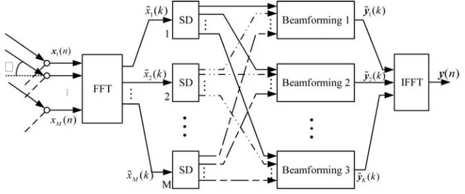
The receive array model of the space-frequency adaptive processing can be regarded as a special case of sub-band adaptive processing, in which the transform domain is the frequency domain, and the transform vector of the sub-band is the Fourier basis vector. An integrated model of sub-band decomposition based on array antenna is given in Fig. 1, where FFT and IFFT (inveres FFT) represent the Fourier transform and inverse transform, respectively. SD indicates sub-band decomposition of the input signal [18].
Consider an SFAP array receiving model utilizingM elements uniform linear array spaceddapart. Generally, the spacing of the array antenna dis half the wavelength of the electromagnetic wave, i.e.,
d= 1/2λ, where λ denotes the wavelength of the signals. In this model, θ stands for the angles with
θ
which the signals enter the array. The data received on them-th array element can be expressed as:
xm(t) = L
i=1
am(θi)si(t) +nm(t) (1)
wheret= 1, . . . , N. On each antenna, there areN−1 delay units to performN points FFT. Assuming that the received signals containL independent signals, the received datax(t) can be written in vector form as
x(t) =A(θ)s(t) +n(t) (2)
whereA(θ) = [a(θ1), . . . ,a(θL)]T represents the steering vector matrix;s(t) = [s1(t), . . . , sL(t)]Tdefines signal vector; and n(t) = [n1(t), . . . , nM(t)]T denotes the noise vector.
In the SFAP model, the antenna array obtainsN samples through A/D sampling, when the GNSS signal is incident on it. The received data on them-th array element can be expressed as
xm = [xm(1), . . . , xm(t), . . . , xm(N)]T (3)
When performing space-frequency adaptive processing, the process of adaptive signal processing is performed in the frequency domain. FFT is applied to the received signals of each array element to obtain the corresponding signals in frequency domain, which can be expressed as
˜
xm(k) =
N
n=1
Znxm(n)e−j2Nπ(n−1)(k−1) (4)
wherexm(n) means then-th sample value received by them-the array element, which represents the time
domain sample value. Since there is spectrum leakage in the Fourier transform, windowing processing is required to suppress the spectrum leakage phenomenon. Znstands for then-th coefficient of the time
domain window function, andxm(n) represents the n-th sample value after them-th array element in
the frequency domain. Rewriting Eq. (4) to vector form can be expressed as ˜xm(K) =fHxm, where
f(K) =
Z1, Z1ej2Nπ(k−1)
, . . . , ZNej2Nπ(N−1)(k−1)
.
3. PRINCIPLE OF SF-SED ALGORITHM
In this section, the specific content of SF-SED algorithm will be divided into three subsections for detailed discussion. The feasibility and computational complexity of the proposed algorithm are also discussed in this section.
3.1. Space-Frequency Domain Sub-Band Processing
Rewriting Eq. (4) into a vector form, the vector composed of M array elements for thek-th frequency point can be expressed as
˜
x(k) = [˜x1(k),x2˜ (k), . . . ,x˜M(k)]T. (5)
The covariance matrix of the frequency domain signals can be given at each frequency point as ˜
R(k) =Ex˜(k) ˜xH(k) (6) There are N covariance matrices as shown in Eq. (6) for the received data of the entire array. In practical applications, the expected estimate of the covariance matrix can be obtained by averaging multiple snapshots. Each frequency point data can be obtained in two ways, which are time domain block receiving data and time domain sliding receiving data. In the simulation analysis of this paper, the method of time domain block receiving data is adopted. Assuming that the number of FFT points isN and that the number of snapshots in the frequency domain isJ, the data of one array element are taken as an example. For the sliding receiving data mode, the received data of them-th array element can be expressed as
The input data required for the FFT operation is
[xm(1), . . . , xm(N)|xm(2), . . . , xm(N + 1)|. . .|xm(J), . . . , xm(J +N −1)] (8)
After sub-band division, each sub-band still contains J frequency domain snapshots. There is no significant difference between the above two methods when dealing with stationary signals. In order to obtain the weight vector, the number of received data required is M×(J +N −1). Therefore, the covariance matrix in Eq. (6) can be solved as the following formula
˜
R(k) = 1
J
J
j=1
˜
x(k)˜xH(k) (9)
Assuming that the received signals and noise are statistically independent and that the mean is zero, the covariance matrix of the array can be decomposed into mutually independent interference covariance matrices, noise covariance matrices, and expected signal covariance matrices. The weight solving problem of each frequency point, according to the linear constraint minimum variance criterion, can be described as the following optimization problem after finding the covariance matrix of each
frequency point: ⎧
⎨ ⎩
min
w w
H(k) ˜R(k)w(k)
s.t.w(k)Hh(k) =Pk
(10)
wherew(k) indicates the weight corresponding to thek-th frequency point on each array element,h(k) a specific constraint condition, and Pk a response corresponding to the constraint condition. Consider
that the GNSS signal power is weak, and lower than the noise power. In order to make the power spectrum flat, the constraint response can be set to a constant. For all frequency points, Pk = 1
is set. According to the Lagrange Multiplier, the law determines that the stability weight coefficient corresponding to the first frequency point on each array element can be expressed as follows
˜
w(K) = R˜
−1h(k)
hHR˜−1(k)h(k), k= 1,2, . . . , N (11)
Therefore, the processed output of the data of the k-th frequency point can be expressed as follows
˜
y(k) =
M
m=1
˜
w∗m(k) ˜x(k) = ˜wH(k) ˜x, (12)
After obtaining the frequency domain output at each frequency point, the inverse time domain output
y(n) = IFFT [˜y(k)] k, n= 1,2, . . . , N.
3.2. Sub-Band Energy Detection and Threshold Structure
In order to reduce the complexity, the SF-SED algorithm constructs a detection statistic in each sub-band to estimate the power level of each sub-sub-band signal and determines whether each sub-sub-band contains an interference signal through a preset decision threshold. Assuming the FFT operation, the input data of the k-th sub-band can be expressed as follows
˜ xk =
˜
xk1,x˜k2, . . . ,x˜kM
T
(13)
where ˜xk1,x˜2k, . . . ,x˜kM represent the frequency domain data of the k-th requency point on the first to
m-th array elements, which contain J snapshots. The frequency domain data of them-th array element of the k-th frequency point can be expressed as
˜ xkm =
˜
xkm(1),x˜km(2), . . . ,x˜km(J)
T
(14)
are consistent because the data difference among array elements is only phase difference caused by the difference of the wave-path. Therefore, the detection statistics only need to use the data of the first array element, which can be expressed as
ηk= i
J
J
j=1
˜
xk1(j)
2
(15)
Considering that the GNSS signal received by the receiver is very weak, its power is much lower than the noise power. When the number of interference signals is limited, and the interference is narrowband, the detection statistics constructed in this paper will be larger in the frequency band where the interference exists. Therefore, by selecting an appropriate threshold value to judge the detection statistic at each frequency point, all frequency bands can be divided into frequency bands with interference and frequency bands without interference. Then weight adjustment and control are respectively performed on each subband. Since the suppressed interference power is significantly higher than the noise power, the threshold can be selected as the average power of the full frequency band after the n-point FFT operation, which can be expressed as
¯
σ2 = 1
N
N
n=1
˜
x21(n) (16)
Since only part of the frequency band contains interference, and the satellite signal power is lower than the noise power, the FFT-converted noise power is recorded asσ2n. It is known that the average power is about ¯σ2n.
At frequencies containing suppressed interference, the average power will be much larger thanσn2. Assuming that each narrowband suppressed interference power level is approximately equal, the power of one interference signal can be denoted as σ2
j, where σn2 <¯σ2 < σj. Each sub-frequency point can be
divided into an interference-containing sub-band and an interference-free sub-band by a threshold ¯σ2.
3.3. Weight Calculation and Complexity Analysis
Although the SFAP algorithm can reduce the partial computation compared with the STAP algorithm, it still needs to calculate the adaptive weight on each sub-band. However, the proposed algorithm classifies each sub-band by the threshold, and the weight will be determined in a targeted manner. For interference-free frequency bands, adaptive interference suppression does not need to be performed. We can perform matched filtering based on the desired signal direction information and only need to give static weights.
For the frequency band with interference, the adaptive processing algorithm needs to be adopted for adaptive interference suppression, then the weight vector of each sub-band can be expressed as
⎧ ⎪ ⎨ ⎪ ⎩
˜
w(k) =a(θ0), ηk ≤σ¯2
˜
w(k) = R˜
−1(k)h(k)
hH(k) ˜R−1(k)h(k), η
k>σ¯2 (17)
where a(θ0) is the space steering vector of the desired signal. θ0 stands for the desired signal arrival direction, which can be calculated by the satellite trajectory. The used adaptive processing algorithm is the PI algorithm, and the constraint vector h= [1,0, . . . ,0]T.
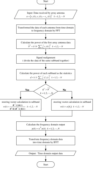
In summary, the steps of the SF-SED algorithm can be summarized as in Table 1. Moreover, the specific algorithm flowchart of the proposed method is shown in Fig. 2.
Table 1. Algorithm steps.
Step1.The array antenna is used for data buffer sampling for a period of time, and the sampled
data is subjected to FFT processing to obtain frequency domain data ˜x;
Step2.Take the output data of an N-point FFT on the first array element, calculate its average
power, and record it as ¯σ2 = 1
N
N
n=1x˜21(n);
Step3.The FFT-transformed frequency domain data is rearranged to obtain data of N sub-bands,
wherein the data of the kth sub-band is recorded as ˜xkm=x˜km(1),x˜km(2), . . . ,x˜km(J)T;
Step4.Calculate the power value of the k-th sub-frequency point as the detection statistic
ηk= J1Jj=1x˜ki(j)2;
Step5.Calculate the weight vector of each sub-frequency point according to Equation (20);
Step6.Calculate the frequency domain output of each subband as ˜y(k) = ˜wH(k) ˜x(k), k= 1,2,
. . . , N, and the IFFT transform is performed on the frequency domain output to obtain
the time domain outputy(n).
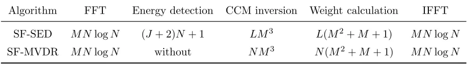
Table 2. Comparison of the computational complexity of the SF-SED algorithm with the SF-MVDR algorithm.
Algorithm FFT Energy detection CCM inversion Weight calculation IFFT
SF-SED M NlogN (J+ 2)N+ 1 LM3 L(M2+M + 1) M NlogN
SF-MVDR M NlogN without N M3 N(M2+M + 1) M NlogN
and the power value of all sub-frequency bands are, respectively, N + 1 andN(J+ 1). (2) For CCM inversion and weight calculation, the conventional SF-MVDR method needs to calculate CCM inversion and weight for all N sub-frequency bands, whose calculational complexity are, respectively, N M3 and N(M2+M+ 1), while for the SF-SED algorithm, only CMM inversions and weights ofLsub-frequency
bands need to be calculated so that the calculational complexities are LM3 and L(M2 +M + 1), respectively. In practice, L N, L < 5 normally when N = 512. Taking M = 4, N = 512, L = 5 as an example, the added computation for the SF-SED algorithm is less than the computational cost which saves in CCM inversion and weight calculation parts whenJ <83 approximately. In other words, the calculational complexity of the SF-SED method is less than that of the SF-MVDR method when
J < 83. In the meantime, the difference of calculation amount may vary more when the number of
antennaM increases. To sum up, compared with conventional SFAP, the proposed algorithm has lower computational complexity.
4. SIMULATION AND ANALYSIS
In this section, simulation results are provided to illustrate the performance of the proposed method. Consider that there is a uniform linear array with 4 antenna elements equispaced byd= 1/2λ. Taking GPS as an example, the L1 frequency is 1.575×10⁹Hz, so dis set as 0.095 m in the simulation. The
sampling frequency fs = 4fc where fc denotes the center frequency of GPS signal. Assume that there
Start
Input: Data received by array antenna
Transformed the data of each antenna from time domain to frequency domain by FFT
Calculate the power of the first array antenna data
Signal realignment
( divide the data of the same subband together)
Calculate the power of each subband as the statistics
(
x k x k1( ), 2( ), xM( )k)
1, 2,k N= ( )( )( )
)
)
)
)
TT = 1, 2,, , Nx
1 2 2
1
1/ N ( ) 1, 2,
k
N x k k N
σ = ⋅∑=⎡⎣ ⎤⎦ = N
2 1 1
1/ J ( ) 1, 2,
k k
j
J x j k N
η= ⋅∑=⎡⎣ ⎤⎦ = N
2
1, 2, ,
k
k N
η >σ = ,,N
steering vector calculation in subband 1
1 H
( ) ( )
( ) 1, 2, ( ) ( ) ( )
k k
w k k N
k k
−
−
= R h = N
h k R h
steering vector calculation in subband
( )0
( ) 1, 2,
w k =aθ k= NN
Calculate the frequency domain output H
( )k =w ( ) k k=1, 2, ,,,NN
y x
Transform frequency domain data into time domain by IFFT
Output: Time domain output data
Start
Yes
Yes NoNo
Figure 2. The algorithm flow chart.
Figure 3. Array pattern of SF-SED algorithm. Figure 4. Spatial response of SF-SED algorithm.
40 45 50 55 60 65 70 75 80
40 45 50 55 60 65 70 75 80 85 90 95
ISR
input(dB)
ISR variation(dB)
SF-SED SF-PI SF-MVDR
Figure 5. ISRout versus input ISR.
40 45 50 55 60 65 70 75 80
40 45 50 55 60 65 70 75 80 85 90 95
ISRinput(dB)
SINR variation(dB)
SF-SED SF-PI SF-MVDR
Figure 6. SINRout versus input ISR.
algorithm, another set of interference signals information is used for simulation in Fig. 4. The DOAs of interferences are −45◦, −25◦, and 20◦, and the normalized frequencies are 0.98, 1.03, and 1. Other experiments are carried out under the same basic simulation conditions as Fig. 3.
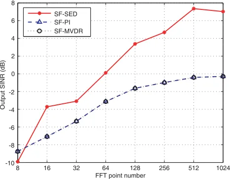
For the simulation parameters of Fig. 3, Fig. 4, Fig. 5, and Fig. 6, the number of points for an FFT operation is 512. The frequency domain snapshot is 64. In particular, the number of FFT points varies from 8 to 1024 for Fig. 7. For Fig. 8, the snapshot number varies from 5 to 80.
-10 -8 -6 -4 -2 0 2 4 6 8
8 16 32 64 128 256 512 1024
FFT point number
Output SINR (dB)
SF-SED SF-PI SF-MVDR
Figure 7. SINRout versus FFT point number.
0 10 20 30 40 50 60 70 80
-2 -1 0 1 2 3 4 5 6
Frequency domain snapshot
Output SINR (dB)
SF-SED SF-PI SF-MVDR
Figure 8. SINRout versus snapshot number.
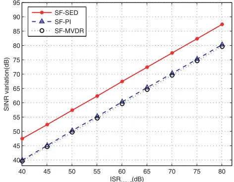
Figures 5 and 6 are the output interference-to-signal-ratio (ISR) and SINR changes versus input ISR, respectively. The ordinate in Fig. 5 is the change in ISR, that is, the absolute value of the difference between the output ISR and input ISR. In the same way, the ordinate in Fig. 6 is the absolute value of the difference between output SINR and input SINR. The two above parameters can be used to represent the influence of the algorithm on the GNSS signals, interference signals, and noise. The two figures show that compared with SF-PI algorithm and SF-MVDR algorithm, the proposed algorithm has larger variation of SINR and ISR. Therefore, the SF-SED algorithm has better anti-jamming performance than the other two algorithms. In addition, according to the simulation result, the output SINR varies with the input ISR, which is because the algorithms solve the weight vectors according to the covariance matrix of input signals. The algorithms have greater suppression of interference reception when the interference power increases.
Figure 7 shows the output signal-to-interference-and-noise ratio (SINR) curve of the proposed algorithm and related algorithms with the change of FFT points. As shown in the figure, the output SINR of the three algorithms increases with the change of FFT points, and the proposed algorithm improves faster. It is because as the number of FFT points increases, the frequency resolution is stronger, and it is possible to suppress the interference frequency more accurately. The SF-SED algorithm uses a static weight vector to process the interference-free frequency band, thereby it forms a main lobe in the desired signal direction and guarantees the satellite signal power. Therefore, it has a higher output SINR than the other two algorithms.
Figure 8 shows the output SINR curve of the proposed algorithm and related algorithms with the change of Frequency domain snapshot. Fig. 8 shows that with the increase of the frequency domain snapshot, the output parameters of the SF-PI and SP-MVDR algorithms are relatively stable, while the SF-SED algorithm is more affected by the frequency domain snapshot. Since the SF-SED algorithm needs to calculate the average power of each frequency point by using the frequency domain snapshot number, the calculated average power is more accurate as the frequency domain snapshot number increases, so the judgment of whether the sub-frequency point contains interference is also more precise. Combined with the simulation results, it can be seen that when the frequency domain snapshot is more than 20, the SF-SED algorithm basically reaches a steady state.
5. CONCLUSION
ACKNOWLEDGMENT
This work was supported by the Natural Science Foundation of Hebei Province (Grant No. F2016501139), and the Fundamental Research Funds for the Central Universities (Grant No. N172302002 and No. N162304002).
REFERENCES
1. Kaplan, D. E. and C. Hegarty, Understanding GPS: Principles and Application, Artech House Publishers, Massachusetts, USA, 2005.
2. Wang, X., M. Amin, F. Ahmad, and E. Aboutanios, “Interference DOA estimation and suppression for GNSS receivers using fully augmentable arrays,”IET Radar, Sonar&Navigation, Vol. 11, No. 3, 474–480, 2017.
3. Chen, Y., P. Chen, and S. Fang, “ Novel anti-Jamming algorithm for GNSS receivers using wavelet-packet-transform-based adaptive predictors,”IEICE Transactions on Fundamentals of Electronics, Communications and Computer Sciences, Vol. E100-A, No. 2, 602–610, 2017.
4. Isernia, T. and A. F. Morabito, “Mask-constrained power synthesis of linear arrays with even excitations,” IEEE Transactions on Antennas and Propagation, Vol. 64, No. 7, 3212–3217, 2016. 5. Hatke, G. F., “Adaptive array processing for wideband nulling in GPS systems,” Proc. 32nd
Asilomar Conf. Signals, Systems, and Computers, 2002.
6. Capozza, P. T., B. J. Holland, and T. M. Hopkinson, “Single-chip narrowband frequency domain excisor for a global positioning system (GPS) receiver,” IEEE Custom Integrated Circuits, 1999. 7. Frost, III, O. L., “An algorithm for linearly constrained adaptive array processing,”Proceedings of
the IEEE, Vo. 60, No. 8, 926–935, 1972.
8. Fante, R. L. and J. J. Vacarro, “Cancellation of jammers and jammer multipath in a GPS receiver,” IEEE Aerospace and Electronic Systems Magazine, Vol. 13, No. 11, 25–28, 1998.
9. Liu, F., M. Zhang, X. Wang, and R. Du, “UCA-NW algorithm for space-time antijamming,” Progress In Electromagetic Research M, Vol. 71, 117–125, 2018.
10. Li, Z., Y. Zhang, H. Liu, B. Xue, and Y. Liu, “A robust STAP method for airborne radar based on clutter covariance matrix reconstruction and steering vector estimation,”Digital Signal Processing, Vol. 78, 82–91, 2018.
11. Lu, Z., J. Nie, F. Chen, H. Chen, and G. Ou, “13 adaptive time taps of STAP under channel mismatch for GNSS antenna arrays,” IEEE Transactions on Instrumentation and Measurement, Vol. 66, No. 11, 1–12, 2017.
12. Compton, T. R., “The relationship between tapped delay-line and FFT processing in adaptive arrays,” IEEE Transactions on Antennas and Propagatio, Vol. 36, No. 1, 15–26, 1988.
13. Fante, R. L. and J. J. Vaccaro, “Wideband cancellation of interference in a GPS receive array,” IEEE Transactions on Aerospace and Electronic Systems, Vol. 36, No. 2, 549–564, 2000.
14. Gupta, I. J. and T. D. Moore, “Space-frequency adaptive processing (SFAP) for interference suppression in GPS receivers,” Proceedings of the National Technical Meeting of the Institute of Navigation, 377–385, 2003.
15. Gupta, I. J. and T. D. Moore, “Space-frequency adaptive processing (SFAP) for RFI mitigation in spread spectrum receivers,” IEEE Antennas and Propagation Society International Symposium, 2003.
16. Chuang, C. and J. Gupta, “On-the-fly estimation of antenna induced biases in SFAP based GNSS antenna arrays,”Navigation, Vol. 61, No. 4, 323–330, 2015.
17. Xu, H., X. Cui, and M. Lu, “Data-oriented calibration method to reduce measurement bias in SFAP-based GNSS receivers,”Electronics Letters, Vol. 54, No. 9, 2018.