Application of canonical correlation analysis ;a comparative study on academic perfomance

APl?LICATION OF CANOOICAL CDRHELATION ANALYSIS '{ "A Comparative Study on AcademicPerfonnance"

BY

'Iuis dissertatiun is submitted in partial fu LfiIrrerrt for the degree of Master

or

Makambi, Kepher Application of canonical

1111111I

KCNYATrA UNIVERSITY, JUNE, 1990.

,DECI J\P.J\TIClN

'Ibis c1issertation is myown work and has not been presented [0r a degree in any other Universi ty.

Signature

.~:

.

KEPEER lillNRY MAKAMBI .

'Illis d.is~3c;rtation has been submitted for examination with my approva.l as University ~)upervisor.

Signature

'l'iLl(~ DeclaraLion

LisL of Contents

i ii iii v ix xi List\of TalJles

Surrrnary 01 Contents AcknowledgerrBnt

OIAI'TER I: INTRODUCITON 1.1 Introduction

1.2 \'.hat is Canonical Correlation Analysis? I.3 Lr-ief Li te ra ture Review

1.4 Aims and Significance of the Study

1

2 5 7

CllAPTER II: SAHPlli CANONICAL CDRRELATION AND CM-DNICAL VAIUA'I'ES.

2.1 2.2

Introduction 9

9 f:8Illple EstimaLes

2.3 Deri vaLion 01 Fundament.al. Equations for

Omonical Correlations and Variates 12

CIIA1YI'ERI II : TI~ST8 OF SIGNIFICANCE AND INTERPRETIVE DEVICES

3.1 Tests of Gignificance Interpretiye Devices

21

26 3.2

Ulwmn IV: APPLICATIONS 4.1 Introduction

4.2 Pesults

37

1.2. L

4,2.2.

4.2. :3

4.2.4

4.2. C)

4.3 4.4

Canonical Correlation Analysis on the

J'elat.Lonsh ip Between Pure Mathematics' "lncl ~"a1..ltematicalStatistics Units (Variables). Cumparative Remarks

Canoui.ca.I Correlation Analysis on the P.elationsbips Between Pure and Applied Mathematics

Coruparative Remarks

Canonical Correlation Analysis on the Relationships Le(;ween Mathematical Statistics and Applied

Mathematics

Comparative Remarks

Ljmitations of the Technique Conclusions

LIST OF REf"ERENCES

38

59

74

76 90 92

93

LIST OF TABLER

TnhIr' J: ~nn~ll.el1'Y2at1sStandard d, eviations and the correlation matrix, R, for scores in Pure

Mathematicsand Mathematical Statistics for

£il~t year, 1984/85

'Iab,le 2: Canoui.ca.lCorrelation Coefficients, weights and loadings for scores in Pure Mathematics

and Mathematical 3Jtatistics for first year,

lU84/85

'IabIe 3: Test Statistics for scores in Pure Mathematics and Mathematical Statistics for first year,

1984/85

Table 4: Cross Loadings for scores in Pure Mathematics

and Mathematical Statistics for first year,

1984/85.

TabJe 5: Samplemeans, standard deviations and the

correlation matrix, H, Jar scores in Pure

Mat.hema t ics and Mathema.ticalStatistics

for first jear, 1985/86

TaJJlc6: Canonical Correlation Coefficients, Weights

ancl Loadi.ngsfor scores in Pure Mathematics and r.lathematical Statistics for first year,

1985/86

39

40

41

44

48

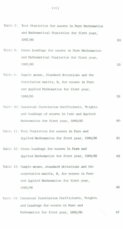
Table 7: Test Statistics for scores in Pure Mathematics and Mathematical Statistics for first year, 1985/86

Tablo 8: Cross Loadi.ngs for scores in lure Mathematics and Mathematical StatisticS for first year, 1985/86

Table D: S~ple rreans, Standard deviations and the Correlation matrix, R, for scores in Pure and Applied Mathematics for first year, 1984/85

Toole 10: Canonical Correlation Coefficients, Weights and loadings of scores in lure and Applied Mathematics for first year, 1984/85

TWJlc 11: Test Statistics for scores in Pure and Applied Mathematics for first year, 1984/85

Table 12: Cross loadings for scores in Pure and

Applied Mathematics for first year, 1984/85

Tabl.e 13: Sample means , standard deviations and the correlaticn matrix, R, for scores in Pure and Applied Mathematics for first year, 1985/H6

TaiJJe 11:l: Canonical Correlation Coefficients, Weights and Loadings for scores in Pure and

Mathematics for first year, 1985/86

50

53

59

60

61

63

66

Tab.lo 15: Test Statistics for scores in Pure and

Applied Mathematicsfor first year, 1985/86 68

Taole 16: Cross Loadings for scores in Pure and

Applied Mathematicsfor first year, 1985/86 71

Table 17: SampLemeans, standard deviations and the correlaU.on matrix, R, for scores in

r:aU1CTTlr':l.tiScatatlistics and Applied

Mathematics for first year, 1984/85 76

Tab1(> U3: Canonical Correlation Coefficients, Weights

and loadings of scores in Mathematical

Statistics and Applied Mathematics for first year

1984/85 77

Table 19: Test Statistics for scores in Mathematical

Statistics and Applied Mathematicsfor

first year, 1984/85 78

TabLo20: Interset Correlations for scores in Mathematical

Statistics and Applied Mathematics for first

year, 1984/85 80

Table 21: Srum)lemeans, standard deviations and the correlation matrix,R, for scores in

Mathematical statistics and Applied Mathenatics

for first year, 1985/86 84

Table 22: Canonical Correlation Coefficients, Weights and .Loadingsof scores in Mathematical Statistics

TabLe 23: Test Statistics for scores in Mathematical

Statistics and Applied Mathematics for first

year, 1985/86 86

Table 24: Cross Loadi.ngs for scores in Mathematical

Statistics and Applied Mathematics for

SUMMARY OF·mN'IENTS

The technique of Canonical Correlation Analysis is useful in

investigating the interrelationships between two or rroresets of

variables. In this dissertation, some interpretive devices in

canonical correlation analysis are used to study the interrelat

ion-ships among different courses offered by the Depar-tment of Mathe

-mati cs, Kenyatta Universi ty.

In section 1.1 of Chapte r I; we give a brief introduction of

Cilllonicalcorrelation analysis. Section 1.2 gives an overview of canoni.cal.correlation analysis whereby the data is assumed to be

from a known population. Section 1.3 outlines some of the work done early on the application of canonical correlation analysis.

TIle aims and significance of the study are given in section 1.4

Nonnally the population parameters are not known and therefore

their sample counterparts are used. Section 2.1 of O1apter II defines the data matrix based on a sample of size N. In section

L.2 the sample estimates of the population parameters are defined.

A rigorous derivation of fundamental equations for canonical

correlations and variates is given in section 2.3.

01apter III outlines the significance tests and

Interpreta-tion of canonical correlations. In section 3.1 the tests of

Si~li£icance of canonical correlations, individual canonical

correlation coefficients and those of particular variables are

discussed. Section 3.2 outlines the interpretive devices used

in canonical correlation analysis.

cor-relat.Lon analysis in studying the interrelationships arrongthe COUl'c;CS ofIered by the Dspartrrerrt of Mathematics, Kenyatta University. SecLlon 4.1 gives the descriptions of the courses which were offered in Erst year 1984/85 and 1985/86 academic years and these courses act as the variables in our current study. Sub-section 4.2.1 of section 4.2 deals with canonical correlation

analysis on the relationship between Pure Mathematics andM athe-matical Statistics and the results for 1984/85 and 1985/86 are both given here. Sub-section 4.2. 2 gives the comparative remarks

on the results of subsection 4.2.1. Canonical Cbrrelation analysis on the relationships between Pure and Applied Mathemat.i.csis dealt with in sub-section 4.2.3 and subsection 4.2.4 gives the comparative

remarks011 t.he results of subsection 4.2.3. 'I11ecanoni.cal.corre la-tion analysis on the relationships betweenMathematical Statistics and Appli.ed Hathematics is given in subsection 4.2.5 andsubsection

11.2.G giyes the comparati ve remarks on the resu1ts of subsection 4.2,:5. Even though this technique (canonical correlation analysis)

ACKNONLEffiEMENT

It gives megreat pleasure to express my gratitude to those

wlto in one wayor tbe other assisted mein the preparation of

t.li is dissertation.

I wish to acknowledgemySupervisor Prof. J.W. Odhiarrbofor

his delLgenceand excellent supervision which he showed by sac

ri-ficiug a lot of his tirre to scrutinise mywork and guide me in the

besL way possible.

I run especially indebted to Mr. L.B.X. Odongoand Mr. Githu

of Kenyatta Universi ty for improving my interest and knowledge in 8LaUstics. Mythanks to Prof. J. Hutio and Dr. E.M. Kukuni

10r providing mewith the data for the present study. I wouId.,

also like to express myappreciation to my lecturers Dr. M.Manene

and Dr. F. Njui for their encouragement during the preparation

01 t.h.i.s work.

I am thankful to Irene Karimi for typing mywork speedily

and wit.li a lot of care.

Finally, thanks to my dear wife, Pamela, for her patience

811(1 cooperation while I workedthrough this project. I also do

apprcc.i.at.e the active suppor-t and encouragement shown by my parents,

CHAPTER I

INTRODUCTION

1.1 Introduction.

In most statistical data analyses, it is usual

to examine linear interdependencies by multiple

regression, which measures the relationship between a

set of predictor (independent) variables and one dependent

(criterion) variable. When observations are taken on a

large number of correlated variables it is natural to

look at various ways in which the number of variables

m i gh t b ere d u c e d w i.tho u t sac rifi.ci n g too m u chi. n for mat ion .

When the variables are regarded as belonging to a single

set then principal components analysis is often

informative.

However, in many research settings, a scientist

encounters a phenomeno~ that is best described not in

terms of a single criterion but, because of its

complexity, in terms of a number of response variables.

In such cases, interest may centre on the relationship

bet wee nth e set 0f criterion v a ria b 1 e san d the set 0f

explanatory factors. In the business or economic fields,

we might be interested in the relationship between a

set of price indices and a set of production indices,

with a view towards, say, predicting one from the other.

In psychological investigations, we might be concerned

with the relationship between a set of personality

on the other. In educational performance investigations,

for example, we might be interested in the relationship

between a group of science subjects and arts subjects.

At university level., one can assess the degree of

relation-ship between a group of Pure Mathematics units on the

one hand, and Statistics or Applied Mathematics units

on the other. Broadly, one is faced with the problem

of investigating and explaining the relationships

between two or more sets of variables. The study of

the relationship between a set of predictor variables

and a set of response variables is known as Canonical

Correlation Analysis

1.2 What is Canonical Correlation Analysis?

In the most general of settings, Canonical Correlation

Analysis describes a multivariate statistical technique

that investigates the degree of relationship between two

sets of variables. It is used in analysing predictor

and criterion variables simultaneOusly. It is particularly

appropriate when the criterion variables are themselves

correlated. When one crtterion variable is available,

Canonical Correlation Analysis reduces to multiple

regression analysis. The use of canonical correlation

analysi's for descriptive purposes requires .no distributional

assumptions. In such cases, the predicto~ and criterion

variables can be measured at the nominal or ordinal level.

To test the significance of the relationships between

canonical variates, however, the data should meet the

of variance.

The Population Model of Canonical Correlation Analysis

Let

r

number of criterion variables and assume p > q. Denote

by ~I= (xl,x2, ... ,xp) the p dimensional vector of

predictor variables, and by YI, = (Yl'Y2?.,yq) the

q dimensional vector of criterion variables. Suppose

that X 'V _Np

C

l::

LXX) and Y 'V Nq

Cl

::

and JI denote the respective mean vectors and _LXX -y

and L are "within-set" variance-covariance yy

matrices defined by

(I.t)

L = E{(Y-~ ) (Y-~ )I}, L > O.

yy - -y - -y yy

We shall use L to denote the "between-set" xy

matrix which is defined by

covariance

= E{(X-~ ) (Y-~ )I}

- -x --y ( 1 . 2 )

If we define a (p+q) dimensional vector, Z, by

then we can view the problem in terms of the partitioned

variance-covariance matrix L_zz given by

r

L

-zz L

LYx

The objective of canonical correlation analysis is to

find a linear combination of the p predictors that

maximally correlates with a linear combination of the

criterion variables. Let the respective linear combinations

be denoted by

a I. X = ( 1 . 4 )

and

(1 . 5 )

The correlation between nand ¢.is given by

a'l: b

xy-( 1 . 6 )

Then out of the infinite number of linear- combinations

between X-variables and the V-variables, we find that

set of linear combinations which maximises the

correlation,

p(!,~).

p(!,~)

scale transformations we choose a and b so that a'l: b - xy

-is maximum subject to the conditions

(i) a'l: a =

xx

-and ( 1. 7)

(ii ) b'l: b = yy

-The value of

p

(!,~)

canonical correlation between X and Y. The corresp

1.3 Grief Literature Review

The theory of canonical correlation analysis was

developed by Hotelling (1935, 1936) as a means of

identifying the most predictable p~variate criterion,

given the availability of several predtctor and

criterion variables.

In fiAance, W~ugh (1942) used canonical correlation

method to measure the changes in prices relative to a

stable value of currency. He did this by taking for

each of the years 1921 to 1940 inclusive, the prices

of beef steers and ~ogs and the per capita consumption of

beef and pork (excluding lard) for the U.S,A.

Shephard and Tanner (1962) used canonical correlation

to study proximities and growth of adolescence, respectively.

In the area of ~ducational ~~rformance, Barnett and

Lewis (1963) used the procedure to analyse qualitative

and quantitative data. Their study was on the academic

prediction. They managed to predict the students'

average grade at the university from the grades on

their GeE A-levels taken (a secondary school examination

required for university entrance), and the student's

average grade at the university was predicted.

In the field of marketing , Perry and Hamm (1969)

used canonical correlation analysis to relate the

degree of social risk and economic risk of 25 consumer

products. They found out that the higher the risk,

importance of personal influence on brand choice.

Psychology is another discipline which has really

utilized the technique of canonical correlation analysis.

For example, Cooley and Lohnes (1971) examined the

association between a set ,of eleven ability-type factors

(for example, verbal knowledge, ~athematics, visual

reasoning) and a set of eleven factors dealing with

career motives (for example, interest in science,

interest in business).

In Ecology, Thornton (1971) applied the method

of canonical correlation to study the effect of complete

rem 0val 0f hip pop 0tam u son g r ass 1 and i nth e Queen Elizabeth

National Park in Uganda. In the study of g"rowth and

development in animals, Tanner, Whitehouse, Marshall,

Healy and Goldstein (1975) applied the method of canonical

correlation analysis in the assessment of skeletal

Illaturity and prediction of adult height.

Further, in psychology, Wingard, Huba, and Bentler

(1979) report a canonical correlation analysis of

relationships between personality variables and use of

various licit and illicit drugs among junior high

school students in a metropolitan area.

Cohen, Gaughran, and Cohen (1979) examined the

relationships between patterns of fertility across 6

different age groups (as dependent variables) and 5

different sets of demographic characteristics as

independent variables (education and occupation;

housing and occupancy) in 5 separate canonical analyses. The units of analysis were 338 New York City health

areas.

Gittins (1979) used canonical correlation analysis

to investigate the relationships between variables of

two distinct but associated kinds in Ecology. He applied

the method to study the connections between the

occurence of plant or animal communities (and their

component speties) and soil or other environmental variables of several areas.

1.4 Aims and Significance of the study

Canonical correlation analysis is a technique

which has not been so widely used in an'alysing

educational performance. In contributing to the few

applications of the technique available, the present

study aims at:

(a) studying the interrelationships among different educational variables, in -particul ar courses

offered by the Mathematics department of Kenyatta

University;

(b) showing how the results of canonical correlation

analysis may be interpreted and the kind of

information provided;

(c) illustrating the kind of opportunities offered by canonical correlation ,analysis in the analysis

of academic data and so contribute towards an improved definition of the role of the method

(d) assessing the ability of canonical correlation

analysis to recover known relationships between

mathematics units of statisti~al interest;

-(e) comparing the results of the analysis for two

consecutive academic years that is, 1984/85

and 1985/86.

Consequently the entire study will

(a) raise many questions on interpretation of results

and thus make more statisticians to venture

into the technique and thus improving its

a pp 1 i cab i 1 i ty ;

(b) act as a reference material for those involved

in studying relationships between educational

variables;

(c) help postgraduate students in statistics to

develop their insight on the usefulness of the

technique;

(d) provide guidance on how.t o make use of existing information (data) to arrive at useful

C1IAPTER II

SAMPLE CANONICAL CORRELATION AND CANONICAL VARIATES

2.1 Introduction

Let ~ be a Cp+q) - component random vector. Let ~1'~2""""

~ be a sRmple of size N from X.

be partitioned into two subvectors

Further, let X , r=1,2, ,N

-r

X(1) of p variables of X and -r

X(2) of q variables of Y; where p+q = n. -r

Thcll

X

-r

[

~

;l)J;

X(2) -r

1,2, ... ,N

where

[Xl,X2, •••.•• , X

J

r r rp

~rp+l'

,

Xm

J

For convenience we will assume p>q.

The observed sample values on the variates may be written

collectively in matrix form as

The Nxn matrix X is called the data matrix of the sample.

2.2 Sample Estimates

X. 1

1 N

-NLX.;

r=l rl i=1,2, ... ,n.

This is the sample mean of the N observations on the ith variable

of X. The vector

represents the n-samp1e means of the n-variables of X. It is

called the sample mean vector. We can write X in the form

x -1 NL X,

N -r r=l

=

lx

\

N

-where 1 is an (Nx1) vector of ones.

Tile sample variance of the ith variable is given by

s

..

1 N - 2

=-NL:(X. -X.) . T'L 1 r=1

;\Ild tile sample covariance between the ith and jth variable; (ifj) is givcu by:

s ..

1 N

-N L (X . - X.)(X . - Xj)

r=l r1 1 rJ

The matrix

s

matrix. Its diagonal elements S.. are sample variances and the 11

off diagonal elements are the covariances. Let the diagonal

matrix of sample variances be given by

then the r-th vector of Standardised variables denoted by Z is

-1'

_1

Z S 2(X - X) -r 6 -1' -'

The varranee covariance matrix of Z is the nxn matrix R, given

-1'

by

R

wncrc

COV(Z(l) Z(2)) -1', -1'

are matrices of orders pxp, qxq and pxq respectively. Note that

the matrix R is the sample correlation matrix.

TIleint.er+rel ationsh.ips within and between the variables

COlllPOSjllg Z(l)

-1' anu -1'Z(2) are specified by the correlation matrix

Usually the variables making up the data matrix are first

standardised to have unit variance so that the variance-covariance

matrix is the correlation matrix.

2.3 Derivation of FWldamental Equations for Canonical Correlations

and Variates.

We now seek linear transformations of each set of variables to

new variates nk and <Pk'the canonical variates, for which the

corroLation matrix has a particular simple and appealing form.

Thus, IvC require that:

(;\) all the _nk be wlCorrelated with one another;

lll) all the _{<Pk be} uncorrelated with one another; and

(c) t.hat the pairs of canonical variates nk, <Pm for k,m ==1,2, ... ,q; be maximally correlated for k==m

and zero otherwi.se,

Let the linear combinations of Z(l)

-r and

Z (2)

-r be

n a1zrl + ......•.... + a z

p rp ==- -ralz(l)

b z +

p+l rp+I + bnmz b- -r' z(2)

where the coefficient vectors

and

bl

...

,

n

The Correlation r, between nand cjJexpressed as a function of

a and b IS

{Var(~'~(1)) .Var(E.'~(2)}~

(2.1)

We rcquire that a and b be such that n and cjJhave unit variances.

That is

Var(n) == aIR a == 1

- 1

1-(2.2)

Var(cjJ)== b'R b == 1 -

22-From equations (2.1)and (2.2)we have

r == aIR b

- 12- (2.3)

Thus the problem is to find a and b which maxirnise (2.3) subject

to (2.2).

Using Lagranges multipliers, we define the Lagrange filllction:

\VhCl'C )" and u are Lagrange multipliers.

To maximise F(~,~,A,]J) we differentiate F(~,E.,A,]J)first

with respect to the elements of a and then those of b. On

setting the results equal to zero we have

ClF

PreJllultLplying(2.4) by (1' and (2.5) by b' gIves

b'R a - ~b'R b = 0

- 21- - 22-

-NO\\I, because'

aIR a = b'R b = 1,

- 11- -

22-equations (2.6) reduce to

From (2.5) we obtain

substi tuting for b In (2.4) we get

III;I( IS

or equivalently

There wil l be a non-zero solution for a in (2.9) if and only

if

o

(2.5)

(2.6)

(2.7)

(2.8)

That is if and only if

IR-1R R-1R - ,2rl

11 12 22 21 /\

°

Therefore 2 ° ° 1 f tJ t ° I'-'I) R-1J'

A lS an eigen va ue a 1e ma rix \" '12 22 '2' .

Let ...... > £2 be the eigen vCllllesof the OILitrix,

ct

then,

The first canonical correlation is rl = £1. Let (1' be the eigen

do .2

vector carrespan lng to £ •

1 Then

n = a'Z(l). 1 -l-r

Similarly, eliminating a from (2.4) and sul.s tiurtiug in (2.5)

gives

0,

that is

IR-IR R-1R - ,2rl

22 21 11 12 /\

o

.

2

Therefore, A is a charasteristic root of the Il1Cltrjx

-1 -1

The number of non-zero characteristic roots of R,,'<'2'(22'<21 and

is tlle same. So again is the maximum characterl

-stic root of Let Q.lbe the corresponding eigen

Thus, the first pair of canonical variables is

= a"Z(l)

"i -:l-r and <PI -1-rb' Z(2)

and the corresponding canonical correlation is rl = 9-1, where

Max. characteristic root of

Max. characteristic root of

and .§l-l and .\2.1 are the eigen vectors corresponding to

9-

i

-1 -1 -1-1

lZll'Z12H22R21and R22R21RnR12' respectively.

The second pair of canonical variables is given by

= a'Z(l)

Tl2 --r and <P₂ = b'Z(2)--r

where a and b are such that [~~Rl2E.is a maximum subject to

In general the (k+l)-th pair of canonical variates is given

= aIZ(I)

Tlk+l - -r and <Pk+l = b'Z(2)- -r '

where a and b are such that ~'Rl2E. 1S a maximwn subject

to

(i)

(iii) (nk+l' ~k+l) are uncorrelated with

(ni'~i) for all i 1,2, ... ,k;

n, = a' .z(1)

1 - 1-r llild ~.

= b~Z(Z)

1 -l-r

Note that the pan (n·, ~.) of canonical variates will satisfy 1 1

cquations (Z.4) and (Z.5) . That is

(Z.lZ)

RZla._-1 - ~RZZb._-1-= 0 (Z .l3)

where a. and b.

-1. -1 are the eigen vectors at the i-th step.

NOIv, nk+l w1correlated with n· implies that 1

It ("011.0I1SFrom (Z.1Z) that

~1'R_2b. O. - --1 -1

Tllrlt is nk+l is uncor'rel ated with ~i as well. Next ~k+l

uncorrclat.ed with <p.

1 implies that

It 101101\'5from (Z.13) that

That is _<Pk+l lS uncorrelated with 11. as well, for all 1

J == 1,2, ,k.

Therefore, the condition that (llk+l'<l>k+l)be uncorrelated

with (lli,<I>i)can be replaced with

~'Rll~i = 0 and Q'R22Qi = 0; for all i = 1,2, ... ,k.

The rroblem can be restated now as

Maximise ~'R12Q

~,Q

subject to

(i)

(ii) b'R b = 1

- 22

-(iii) a'Rlla. == 0; i == 1,2, .•..•,k

- -1

(iv) 1,2, ... .k,

UsillgLagranges multipliers, let us difine

F(i.~,~,A,lJ,~,i=D= ~'R12E. - A/2(~'Rll~ - 1)

k

- \J/2(Q'R22

Q

-

1"=1 k

- L 8. (b'R22b.)

i=l 1- -1

(2.14)

Differentiating (2.14) with respect to a;b,A,\J,()',.and 8. respecti

-- - 1 1

vely and equating the results to zero we obtain

aF

-= 0

o

_dF __ :=

dA 0 ~'Rll~ := 1

o

=

aF

I"~. I

0, i

o

()F

----_{;)f) .}c= () ~ ,R2 2)21'.

.L

0, i 1,Z, .•.••• ,k.

Pr-emul tipJying (2.15) by a'.; for fixed J

- J we get

which implies that

O:j = 0, Vj = 1,Z, •...•• ,k.

SimiJarly, premultip1ying (2.16) by b., for fixed j we get

-J

b'.;R21a - ub ' .RZZb - e.b ' .R2Zb. := 0

- J - - J - J- J -J

wliich implies that

G.

J 0, V.J = 1,Z, ••••• ,k.

TllUS, the system of equations reduces to

a'R a:= 1

- 11

-b'R b:= 1

-

ZZ-(2.16)

(2.17)

which are the same as equations given originally, Therefore, the

(k+l)-th pair of canonical variates 1S

= at Z(l)

nk+l - k+l-r and ¢k+l = -b'k+l-z(Z)r

wherc ~k+ 1

-1 -]

HJ \ HlzRnRn and ~k+1

Z -]-1

.Q 1\-1\ ill RZZRZlRliRlZ'

1S the eigen vector corresponding to _!I.Z_k+l 1n

is the eigen vector corresponding to

CHAPTEH III

TESTS OF SIGNIFICANCE AND INTERPHETIVE DEVICES

3.1 Tests of Significance

For purposes of testing hypotheses we shall

assume that the observations are obtained from a normal population.

(a) Joint Nullity of all the q Canonical Correlations

We know that -1

2

canonical correlation coefficient. It is often necessary to test the simultaneous departure of the canonical

correlation coefficients from zero. Joint nullity of

all the q canonical correlations would indicate the

absence of any linear relationship between the two or more sets of variables. Suppose that we wish to test

the null hypothesis that, say, the X-variables set is uncolrelated with the V-variables sets that is,

where

Hl: Pk

t-

01' equivalently

H _L12 = 0

0

a qainst

H 1 : _L12 t 0

where _L12 is the matrix of intercorrelations. Then

=

wltere A is the Wilks' Lambda statistic. The range of

A is 0 to 1. It is apparent that A may be regarded

as tile product of the proportion of variance left

unexplained by the q canonical correlations. We see that if there is little correlation between the two

sets of varables, A will be close to unity, while if

they are closely correlated A will approach zero. 8ortlelt's chi-square approximation for the

disLribution of A is

X2 -~-HP+q+3D10geA.

Under the null hypothesis x2 is distributed approximately as a chi-squared variable with pq degrees of freedom

asymptotically as N -+ 00 The hypothesis is rejected if

where a is the size of the test. If the null hypothesis

(no relationship) can be rejected, the contribution of

the first pair of canonical variates can be removed

fro III A and the stat istic a 1 s i 9 n i f i can ceo f ,the rem a i n i n g

pairs of canonical variates assessed. It is generally of interest to remove the contribution of the largest

roo t , the fir st two roo t s, and soon? from .A and the n

to assess the significance of the remaining canonical

(b) Joint Nullity of the Smallest q~k Canonical

Correlations

A general criterion for testing the joint nullity of

the canonical correlations is given

by

q 2

II (l-r.)

. k 1

1=

The significance of Ak may be assessed by the chi~square

appro x iIIIation gi ven by

where x2 is distributed approximately as a chi-squared

variable with (p-k+l )(q-k+l) degrees of freedom. Ak

provides a test of the residuals after the effects of

the preceding correlations have been removed.

This test will eventually give us the number of

useful and interpretable canonical variates. It is

generally accepted that if the overall test is significant

then rl at least must be significant. The significance

itself is usually never directly tested,

of

(c) The Significance of Individual Canonical Correlation

Coeffi ci ents.

An alternative to the likelihood ratio tests of the

hypotheses considered above is arrived at through the

arplication of Roy's union intersection procedure. In

this context we write the multivariate hypothesis.

= p =

a

q

against

as an intersection of composite univariate hypotheses

and as a union of corresponding alternative hypotheses

respectively, that is

H :

o (\_{a, b}(p(a_-,_-b) = 0)

against

L

J

a, b

wh ere fJ(~,~) is the simple correlation between nand

q) (tile linear composites a'z(l) and b'z(2)

-r r

respectively).

The test criterion for the hypothesis above is

the square of the maximum attainable correlation between

the linear composites a'z(l)

- -r and -b'z-r(2) for all

choices of a and b subject to the normalisation

~'Rll~

I

b 1 . This quantity is the

condition = _E.R22 =

largest root, _{r 1 '}2 of

- 1 R21

-1

R12

A

2y~

(R22 _{R 1 1}

-

The significance of rl2 may be tested by referring

it Lo critical points of the greatest characteristic

roaL (gcr) distribution defined as follows:

Let

Le two independent Wishart matrices. Then the cIa r q e st

- 1

eigenvalue

e

Note that e can also be defined as the largest root of

the determinantal equation

Iv

-

e

(v

+v

I

a .

If A is an eigenvalue of

v

1

-1

eigenvalue of (Vl+V2) V2. Since this is a monotonic function

of A, 0 is given by

where

Al

1+Al

is the largest eigenvalue of

e

Clearly, since

Al > 0, we see that

a

rherefore, the null hypothesis is accepted at the

level a if

and rejected otherwise. Here ea(q,ml ,m2) is the upper

lOOa percentage point of the qcr distribution with

parameters q , ml = (lp-ql-l)/Z and mZ = (N-p-q-2)/Z'

If the overall hypothesis of independence given above

is rejected, the signific~nce of the kth root may be

tested (k=Z, ... ,q). The procedure is identical to the

overall test using r~, but an adjustment to the first

degree-of-freedom parameter however is r equir e d . The

parameter qk is given by qk = min(p-k+l, q-k+l).

(d) The Contribution of Particular Variables

The significance of the contribution of particular

variables to the can o nic al relationship can be tested by a

modification of the likelihood ratio test procedure

described above. The test is accomplished by comparing

interest are first included and then omjtted. The value

of A is first calculated from

A =

q 2

II (l-rk)

k=l

with all the variables included. Now, suppose K X''s and

1

K2 Y's are omitted. The value of A is then reca

lcu-lated for the remaining (p-kl) plus (q-k2) variables. Denoting this second value by A*, the quantity

X2 = -

~-

!

(

iJ

*

is distributed approximately as a chi-squared variate with {p-kl )(q-k2) degrees of freedom. The test statistic is then given by

which has an approximate chi-square distribution with

3.2 INTERPRETIVE DEVICES

(a) Canonical Correlation Coefficients (rk)

These are product-moment correlation coefficients

between the kth pair of canonical variates, nk and ~k'

They can also be interpreted a~ multiple correlation

coefficients between a particular canonical variate of

one set and the complete set of variables of the other. The magnitude of rk expresses the degree of linear

correlation between nk and ~k' They are dimensionless

or both sets.

A squared canonical correlation coefficient,

represents the ratio of two determinants or generalized

variances - namely the ratio of the generalized total

variance. The sq~are of a canonical correlation is also

interpretable as the overlapping variance between the kth

pair of canonical variates. It should be noted that

canonical correlation coefficients calculated from the

sums of squares and product matrix, the variance-covariance

matrix and the correlation matrix for a particular set of

data are the same.

rhe magnitude of the sample correlation? _does

depend to a large extent on the relative number of

variables and sample involved. As the number of variables,

(p+q), approaches the sample size N, the value of rl

(the first canonical correlation) tends rapidly to unity.

When (p+q) ~ N one or more canonical correlations of

unity will inevitably arise.

Apart from measuring the relationship between

canonical variates, canonical correlations have two other

r-irstthey provide an indication of the dimensionality

of linear relationship between the measurement domains.

uses.

That is,they help in determining the number of useful and

interpretable canonical variates. _{Secondly, they are used}

(b) Canonical Weights

These are elements of the vectors _~k and E.k .

They serve to transform the original variables so that

the correlation between the two sets of variables i s

maximal. The magnitude of the weight tells us the

imp 0r tan ceo f a va ria b1e fro m 0n e set with regard to the

other set in obtaining a maximum correlation between

the sets.

'1:1enumerical va 1ues of canonical wei ghts depend on

the selection of variables as well as on their scale.

Addition or deletion of variables in either set is likely

to produce major alterations in the remaining coefficients.

Standardising the observed variables to zero mean and unit

variance will remove the scaling effects but the inter

-dependencies still remain.

As in multiple regression, the canonical weight

coefficients may be highly unstable due to multicolli~

nearity. Thus, some variable may have a small or even

negative weight because the variance in the variable has

already been accounted for by some other variable(s).

The adverse effects of collinearity on the algebraic

sign .ind ma qn itude of the canonical weight coefficient

give a rather warped view of the relevance of the

variables.

(c) Canonical Loadings (Intraset Correlation Coefficients)

A canonical loading (an intraset correlation

of the original variable and its respective canonical

variate. Thus, it reflects the degree to which a variate

is represented by a canonical variate. More precisely,

a cllnonical loading gives the correlation between a

can 0nic a1 va ria tea n d a n 0b s e r v e d va ria b1e of the same set.

There are two sets of intraset correlations cor

re-sponding tq the two measurement domains. The vector of

canonical loadings associated with the kth canonical

variate can be obtained by premultiplying the vector of

canonical weights by the appropriate matrix of within=set

correlations. For the variables and canonical variates

of z(l) the canonical loadings are given by

-r

corr(~~l), nk) = corr(~~l), ~Ik ~~l))

l

~

)

J

'

I

N -r -r -k

r=l

Rll ~k

=

=

= ~~l) (say), (3. 1 )

wher-e ,(1) is the

-k

k-th canonical

pxl vector of correlations between

the va riate 0f z( 1 )

-r and the observed variables of z ( 1 )

-r

Similarly, for the V-variables set we have

Corr(z(2) ,¢ ) = R b = £(2)

-r k 22 -k -k (say) ( 3 .2)

(d) Cross Loadings (Interset Correlation Coefficients)

A cross-loading gives the relationship between an

obseNed variable from one set with a canonical variate

There are two sets of cross-loadings corresponding

to the two measurement domains. For the correlations of"

the variables of

z(2) we have

( 1 )

z with the canonical variates of

= Corr(z(l), b' z(2)) -r " -k-r

I

-,-~1)~~2l~k

1 N

L: N r=l

(say) ( 3 .3)

where is the pxl vector of interset correlations

bet wee nth e k - t h can 0n i c a 1 va riate, '~'k'0f z (2 ) and

the observed variables of z(l)

From equation (2.4) it is easily seen that

( 3 .4)

Thus, cross-loadings can be obtained by taking the

product of the canonical correlation coefficient and

the canonical loading.

In a similar way,

E(yn) (say)

-k ( 3.5 }

where E(yn) is the qxl vector of correlations between -k

the k-th canonical variate, nk' of z(l) and the

observed variables in ~(2).

The attractive feature of cross-loadings is that

separately with the canonical variate from the other set.

The cross-loadings are more conservative, less inflated

than within-set ·loadings.

(e) Proportion of Explained Variance (Variance Extracted by a Canonical Variate)

The proportion of the total variance of a measurement domain which is associated with a canonical variate is referred to as the variance extracted or accounted for by

the variate. It is an index of the extent to which a

canonical variate explains the total variance of the

domain of which it is a linear composite.

The variance extracted by a canonical variate is

assessed as the sum of squared loadings on a variate'

divided by the number of variables in the set.

The proportion of explained variance in the X-set

variables that is accounted for by a particular

canonical variate is given by

= P_{E E'k/}2

i=1 1 P

(3 .6 )

2

R(k)x denotes the proportion of variance in the

x-set variables accounted for by a particular canonical variate Efk is the ith squared intraset correlation with nk,

that is, the kth canonical variate. Similarly, the proportion of variance in the V-set accounted for by a particular canonical

2

variate, denoted by R(k)y' can be computed by

2 R(k)Y =

q 2

E Ehk h=1

1\ pair of canoni ca1 vari ates may extract very di fferent amounts

of variance from their respective sets of variates.

Because canonical variates are independent of one another

(orthogonal), percentages of variance can be summed across

variates to arrive at the total variance extracted from

the variables by all significant canonical yariates.

(f) Red u n dancy

Hedundancy is the proportion of the total variance

of a l1Ieasurement domain predictable from a linear

composite of the other domain, given tHe availability

of the second domain.

The redundancy, R2 of z (1 ) with respect to

(k)x/y'

the k-th canonical variate _¢k = b' z(2 ) of ( 2 )

-k - z ,

given the availability of _~ (2)

_,

of the squared interset correlations (cross-loadings)

between the elements of z(l) and ¢k' That is

R2

(k)x/y =

P 2

L: Eik/p

i=1

( 3.8)

where Eik

of z (1 )

is the correlation between the ith variable

and the k-th canonical variate of z(2 ).

Similary, the redundancy, R~k)Y/X' of z(2).

given the availability of z( 1 ) , is given by

2

R(k)Y/x =

q 2

L: Ehk/q

h=l

( 3 . 9 )

where E..hk

of z(2)

is the correlation between the h-th variable

Alternatively, redundancy may be regarded as the

product of the within-set variance times the between-set

variance accounted for by a canonical variate. In other

words, redundancy is the product of the variance extracted

by a canonical variate from its own domain times the

the variance which the canonical variate shares with its

counterpart of the domain. Thus, we write

R2 ₌ 2 2

R(k)x rk

(k)x/y

for the redundancy of z( 1 ) , given the availability of

the set z( 2 ) , and

2 R(k)y/x

ror the redundancy of z(2)

=

given the availability of

( 1)

z .

In more general terms, redundancy answers the

question~ If I knew the score on a canonical variate

fr o m one set, how much would my uncertainty regarding the

other set be reduced? It is possible, for instance, for

a can ani ca1 va ria te fro man e set tab e ani m par tan t

dimension in its own set of variables, but correlated

with an unimportant di.mension among the other set (and

vice versa). Therefore the redundancies for a pair of

canonical variates are not usually equal. That is

R2 :f

(k)x/y

2

R(k)y/x

Because canonical variates are orthogonal,

across canonical variates to get a total for the

variables and, thus, a total redundancy measure for

one set relative to the other, and vice versa.

For the total redundancy in the set _z( 1 ) _{, given}

the canonical variates <Pl,<P2' '" '<Pm

2

R(T)x/y

m

=

R2

(k)x/y (3.10)

where m is the number of retained canonical variates.

Similarly, the total redundancy in !(2), given

the canonical variates nl' n2' ... , nm of z(l) is

given by

R2

(T)y/x =

m q

L (L Ehk/q)

k=l h=l

m

= L

k=l R2

(k)y/x (3.11)

T his inde x pro v ide san 0ve r all measure of the variance

explained in one vari~ble set by the variables of the

other. Total redundancy is asymmetric between domains,

to that in general

R2

J

(T)xjy R(T)y/x

(g) Variable Communalities

(i) Intmset Variable Communalities

These are the proportions of variance accounted

own set.

These are obtained as the sum of squared intraset

correlations (loadings) between a variable and the

retained canonical variates. For the i-th variable of

(1)

z , the intraset or within-set communality, h2 . ,

Wl

is therefore

(3.12)

where €ik is the intraset correlation of the i-th variable

with the k-th canonical variate of z(l).

Similarly, for the within-set communality of the h-th variable

of z(2), we have

= (3.13)

(ii) Interset Variable Communalities

These are the proportions of variance accounted for

". by the retained' canonical variates of the other set.

They are obtained as the sum of squared cross

loadings (interset correlations) between a variable and

the retained canonical variates. The interset or

between-set communa 1 ity, of the i-th variable of z( 1 )

with the retained canonical variates of z(2) is therefore

given by

= (3.14)

where is the interset correlation of the i-th

variable of z(l) with the k-th canonical variate

Similarly~ the interset communality of the h-th

variable of

ofz(l) is

(2)

z with the retained canonical variates

= (3.15)

CHAPTER IV

APPLICATIONS

r4.1 INTRODUCTION

This chapt.cr is aimed at applying the teclmique of Canonical

Correlation AnaIysis to data on scores of students in Mathematics

]Jl first ycar for two consecutive academic years, that is, 1984/85

allc1 1985/86 academic years. Six cases on the applications are

discussed. The various fields of Mathematics, namely: Pure

Mat.hcmatics, Statistics and Applied Mathematics, provided the three sets of variables for the analysis, whereas the units within each

field formed the specific variables. The three sets are each

characterized by N observations, where N is the same for each

academic year (for 1984/85 academic year, N = 66 and for 1985/86,

N == 44). The number N represents the actual number of students

\\lJIO sat for the examinations in a particular academic year. The

tlrrcc sets of variables are denoted by X,Y and Z, where the

X-variables set represents scores in Pure Mathematics, the

Y-variables set represents scores in Mathematical Statistics and

t1le Z-variables set represents scores in Applied Mathematics. The

variable sets are as given below:

(a) X-Variables

Xl - Calculus I

X - Calculus II

2

X3 - Linear Algebra I

(b) Y-Variab1es

Y1 - Probability wId Statistics I

Y2 - Prababi1ity mid Statistics II

(c) Z-V'8.riah1es

Zl - vector Analysis

Z2 - Classical Mechanics.

4.2. R[SULTS.

4.2.I• CANONICAL CORRELATION ANALYSIS ON THE RELATIONSHIP BETWEEN

PURE MATllEMATIC AND MATHEMATICAL STATISTICS UNITS (VARIABLES) .

This will be split into two analyses:

(I) 1984/85 academic year

(II) 1985/86 academic year

(I) 1984/85

'I'abl c 1 below gives the sample means, standard deviations and

the correlation matrix,R, for scores in Pure Mathematics and

Mathcmatical Statistics for first year, 1984/85 academic year.

Tahle 1: Sample meWIS, standard deviations and the correlation

matrix, R, for scores in Pure Mathematics and Mathe

Variable Mean Standard deviation

Xl 58.3 11.6

X2 65.3 10.3

X3 68.5 13.9

X4 67.0 8.0

Yl 62.4 12.7

Y 62.3 8.6

2

1.0000 0.4222 0.5652 0.3148 0.6047 0.3102

R = 0.4222 1.0000 0.5589 0.3022 0.3291 0.3534 0.5652 0.5589 1.0000 0.3914 0.5798 0.3429

0.3148 0.3022 0.3914 1.0000 0.4922 0.4143

0.6047 0.3291 0.5798 0.4922 1.0000 0.4005

0.3102 0.3534 0.3429 0.4143 0.4005 1.סס00

Canonical Correlations

Table 2 below shows the canonical correlation coefficients (rk)

and.other indices, for first year 1984/85. The first canonical correlation, rl, is 0.737 representing about 54% (r/

=

The second.canonical correlation, r2, is 0~260 which represents

about

n

TabJe 2: Canonical Correlation Coefficients, weights and

loadings for scores in Pure Mathematics and

Mathematical Statistics for first year, 1984/85.

eigen- Canonical Canonical Weights and Loadings

K value, correlation,

Pure Mathematics Statistics

2 (X-Variables) (Y-Variables)

r rk

k

Weights Loadings Weights Loadings

1 0.543 0.737 0.485 0.821 0.866 0.971

-0.036 0.512 0.261 0.608

0.379 0.803

0.436 0.726

2 0.068 0.260 -0.564 -0.279 -0.664 -0.239

0.964 0.600 1.060 0.794

-0.504 70.082

0.515 0.432

Number of Significant Canonical Variates (Dimensionality)

III order to fi1ld the number of significant canonical variates,

we test the overall null hypothesis

against

The cOJilputedchi-square,

x~

,

for various degrees of freedom appear in table (3) below.

Table 3: Test Statistics for scores in Pure Mathematics and

Mathematical Statistics for first year, 1984/85~

K X2 2 2 d.£.

c \0.01) \0.05)

I

I

2 4.378 0.115 0.352 3

13art1cttIS X2 statistic given in the table provides tests of the

joint nullity of the residuals after the larger roots are succes

-sively removed. From the table we see that

for all rk(K = 1,2).

Thus, the null hypothesis of independence is rejected (for a= 0.01

awl O, OS) . Consequently, the two canonical variates are required

to [ulJ)' account, for the relationships which are present between

the X- and Y-variables. Therefore, a dimensionality of 2 is

required to study this relationship.

Canonical Weights.

These are also given in Table 2 above. From the table we see

that the first canonical variate is associated with ~ and X4

implies that Xl and Yl contribute more towards the first canonical

co rrclation than all the other variables.

The sccond canonical variate is associated with X2 in the

X-Vel riabIes set and Y2 in the Y-variables set. Thus, X2 and Y2

contribute more significantly towards the second canonical corre

-lation.

Canonical LoacLings (lntraset Correkat ions )

----

--The canonical loadings also appear in Table 2 above and are

hclpful in establishing the nature of the canonical variates

defined on each set of variables.

The correlation of the X-variables with n1

=

~i'

:

~

alike in sign. The variable Xl shows the strongest correlation

(0.821) with

n

,

variate nl shows that the performance in all the X-variables is

correlated though to varying extents. Thus, it is possible to

Eet a Linear combination of these variables.

The lorresponding correlations of the Y-variables with

cf>= Ij"z(2) have the same sign, indicating also that the per

-l -1.

-fOl'lllancin thc e two variables comprising the Y-variables set is

corrclated. The variate cf>lis mainly represented by Yl with a

correlation of 0.971.

The first pair of canonical variates, (nl'cf>l)'indicate that

.xland Yl contribute most significantly to the first canonical

correlation. This implies that the performance in Xl and Yl should

be most highly interrelated, a fact that is established from

as 0.605 whidl is the highest correlation between the variables.

Further, these units (variables) account for most of the variance

in their respective variates.

Turning to the second pair of canonical variates we see that

the correlations tend to be smaller than those of the variables

with .'11 and <Pl' The loadings of the X-variables with '1Z vary in

Slgll. The canonical variate I1Z appears to represent XZ(0.600)

wh irh is least correlated with 111, However, we notice that Xl

and X3 (the variables which are highly correlated with '\) have

negative correlations with nZ' Similarly, the loadings of the

r-var Iablcs with <PZvary in sign. jvbreso, <PZis largely repre

-sentcd by YZ(O.794) wh ich has the least correlation with <PZ'

It should be clear that the first canonical variates, n1 and

cjll' telldto represent those variables whose performance is most

lughly correlated.

The fact that Xl and Yl contribute more to the first canonical

correlation is consistent with the interpretation given by the

canonical weights above. Further, X

z

the second canonical correlation as also given by the canonical

weights. Therefore, we can assume that the canonical weights

given in this analysis are quite stable (their interpretation

is valicl).

Cross Loadings (Interset Correlations)

These appear in Table 4 below. These loadings are helpful

of variables. From the table we notice that all the X-variables

are directly related to <Pl' However, Xl seems to be more corre

-lated with <Pl' Further, Y 1 is more correlated with nl (0.7l5) than

Y2(0.448) .

Table 4: Cross Loadings for scores in Pure Mathematics and

Na therna.itcal Statistics for first year, 1984/85.

!

,.-<P2 <P2 Tll nZ

--

-Xl 0.605 -0.073 Yl 0.7l5 -0.062

X2 0.377 0.156 _Y2 0.448 0.206

X3 0.592 -0.02l

X4 0.535 0.112

Thus, it is clear that Xl and Yl contribute highly to the

first canonical correlation (composed with the other variables) .

This confinns the fact that the perfonnance in Xl .in more

related to that of Yl' That is, students who performed well in

Xl tended to do the same in Y1 .

Two of the X-variables vary inversely with <P2' Nonetheless,

cP2 and n2 tend to identify the interrelationship between X

z

Variance Extracted oy Canonical Variates

The proportion of explained variance in the X-set variables

that is accowlted for by the first canonical variate,

n

'"0.527

Thus, the first canonical variate, nl, explains about 53% of .

tlletotal variance of the X-variables set.

Next, the proportion of variance extracted by the second

canonical variate, n2, in the X-variables set is

'"0.158

which is about 16% of the total variance. Therefore, the two

canonical variates accowlt for about 69% of the total variance

in Lite X-variables set.

Considering the Y-variables set, the proportion of variance

accounted for by the canonical variate, cjJl'is

~ 0.344.

Thus, the two variates account for almost 100% of the variance

ill thc Y-variables set.

Redwlu3ncy:

The redwldancy in the X-variables set generated by each of

R2 (l)x/y

and

R2 (2)x/y

respectively.

2 2

R(l)x r1

0.527 x 0.543

0.286

0.158 x 0.068

'"0.011

}\lsothe redundancy in the Y-variable set attributable to the

canonical variates nk (k = 1,2) 1S

R2 (l)y/x

and

R2 (2)y/x

respectively.

= 0.656 x 0.543

'"0.356

0.344 x 0.068

'"0.023

From the above calculations, we notice that a higher proportion

of variance in the Y-variables set is predictable from the X-variables

set than that of X-variables set predictable from Y-variables set.

given the Y-variables.

From the redundancies given above, it is clear that <PI (which

mainly represent Yl) accow1ts for a greater part of the e2q1lained

variance of the X-variables. Also nl (represented mainly by \)

accowlts for a higher proportion of the explained variance of the

Y-va.riablcs.

TJlC two canonical variates illand T12 account collectively for about 29% of the variance in the Y -variables set, whereas

1']cl" :::1,2) account for about 38% of the variance in the X-variables

set; that is

R2

'" 0.29

(T)y/x

and

R2

'" 0.38 (T)x/y

respectively.

(11) 1985/86

Table 5 below shows the sample means, standard deviations

and the correlation matrix, R, for scores in Pure Mathematics

Table 5: Sample means, standard deviations and the correlation

matrix, R, for scores in Pure Mathematics and

Mathematical Statistics for first year, 1985/86.

Variable Mean Standard deviation

Xl 58.8 9.9

X2 53.6 14.0

X3 69.8 11.7

X4 77.4 13.7

Y 60.8 8.9

1

Y2 64.3 6.9

1.0000 0.4554 0.4467 0.5603 0.5133 0.3044

R = 0.4554 1.0000 0.2862 0.6244 0.5569 0.4755

0.4467 0.2862 1.0000 0.4131 0.3163 0.3756

0.5603 0.6244 0.4131 1.0000 0.4870 0.6988

0.5133 0.5569 0.3163 0.4870 1.0000 0.4559

l

__

CanonicJ.lCorrelations

TJ.ble6 below gives the canonical correlation coefficients

(lk' k = 1,2), the canonical weights and loadings for scores in

J\llC Mathematics and Mathematical statistics for first year, 1985/86.

The first canollica1correlation, rl, is given as 0.749 which

2

palf of canonical variates. The second canonical correlation, r2,

2

is 0.4(18 representing about 22% (r2 = 0.219) overlapping variance

beth"cen the second pair of canonical variates.

TabJ(' (I: Canonical Correlation Coefficients, Weights and Loadings for scores D1 Pure Mathematics and Mathematical Statistics

for first year, 1985/86.

--- - .

Ligell- Canonical Canonical Weights and Loadings

value, Correla

-K Pure Mathematics Statistics (Y-variables)

2 tion, (X-variables) r

k _rIc

Weights Loadings Weights .Loadings

1 00561 0.749 -0.051 0.573 0.383 0.732

0.278 0.771 0.766 0.940

0.182 0.546

0.743 0.963

2 0.219 0.468 -0.957 -0.624 -1.056 -0.682

-0.664 -0.422 0.822 0.341

0.142 -0.055

1.020 0.128

-

-Uuncus 1.0Jtal ity

To determine the number of significant canonical variates, we test

jstile i.nt ercor relat i.on matrix between the X- and Y-varia

-12

blos. Tahle 7 LeLow repotts the computed chi-square,

x~

,

t.ab Ie ("iJ i-square, x~, values for various degrees of freedom. These

,1)'(' 11(_'C(~:-;s;lry for t.c st.ing the above hypo the si.s,

1:)'0111 the table we see that

X2 > X2. for all k = 1,2

c a'

Test Statistics for scores in Pure Mathematics and

Mathematical Statistics for first year, 1985/86.

I, X2 2 2 _d.f.

X(O.Ol) X(0.05)

c -- ---"

I 42.29 1.65 2.73 8

2 fJ.77 O.llS 0.352 3

--_.. _'

-Till' Il'

r(

["'"0 lcvrl s of si.gn iLicance , a = 0.01 and 0.05. This suggests that

liJr' two canonical variates are required to account for the rela

-r i(III';iIjI'S which are present between the two variable sets.

Canouical WeigHts

The canollical weights are given in Table 6 above. We notice

tklt .the first canonical variate, n1, is associated with X4 which

n~p)"I'S('II L 1'1 more than YI' Therefore, X4 and Y2 contribute more

t.ownrds obtaining t he first canonical correlation than all the

0111('1' vnriabl cs makiug up the two sets.

'Ihl' second canou i.ca.l variate, ~n2'1S associated with X4with

,

I \

\"

(,r

th.: f Xtj' Xj and YI contribute most significantly towards the

5C((1l1dcanon icul, correlation.

Canoi1i.cal loadings

All the X-variables contribute in the same direction to the

fil'sL ca1lonical variate,nl, (see Table 6 above) and all have

sizeable correlations with this variate. Above all, .nl seems

to he an expression of X4(O.963).

The correlations of the variables wi.th 112 are noticeably weaker

t.hnn thci r correlations with n1; the strongest correlations being

01' X1l-O.624) and X2(-O.422). Accordingly, n2 may be

It can also be seen from the tahl.e rC)',::ll't.ktl as an expression of Xl'

Lhnl t.hroo varl ahles , Xl' 1\2 and X3 are inversely related with

"

a

COIISj clering the canonical variates (~k= ~~ ~ (2) (k=L, 2) of

Y-v:lri(ll>les, we see that t.he two variables making up this set

con tribute in the same direction to <PIand the correlations are

quite high. The strongest correlation with <PI is that of

l'2(O.940). The second canonical variate, <P2' is largely

The first pair of canonical variates, (nl,4>l)'indicate

that X4 and Y2 contribute most heavily to the first canonical

correlation and accordingly the performance of students in the

two va riablcs is more correlated than to the rest of the variables.

We uot.c , from the correlation matrix, R, that X4 and Y2 have the

highcst correlation of about 0.699.

Tllc second canonical variates,

"

z

COil tributc more to the second canonical correlation. From the

correlation matrix, R, Ie notice that the correlation of Xl with

Yl is 0,513 \\'11i.ch.is the second largest after that of X2 with

)"1(0,557), However, the difference between the two correlations

is not very significant.

Whereas the interpretation that X4 and Y2 contribute more

significantly to thefirst canonical correlation is consistent in

bot.h the canonical weights and loadings, the canonical weights and

loadillgsdo not tally in their interpretation of the second pair

canolliculvariates. That is, according to the canonical weights,

X4 alldYl contribute more to the second canonical correlation

whereas the canonical loadings identify ~ and Y1 as the most

important variables. However, we nonnally tend to prefer the

jnterpretation given by the canonical loadings.

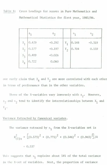
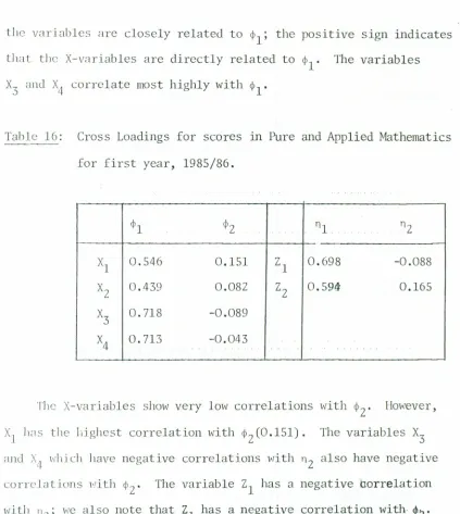
Cross Loadings

FrolllTable 8 below, we see that all the X-variables are directly

related to 4>1' The strength of the relationships does not vary so

much ; that of X4 is highest (0.722) and X3 the lowest (0.409).

Table 8: Cross Loadings for scores in Pure Mathematics and

Mathematical Statistics for first year, 1985/86.

<PI <PZ nl _nZ

Xl 0.4Z9 -0.Z9Z Yl 0.548 -0.319

X

z

X3 0.409 -0.OZ6

X4 0.722 0.060

our early claim that X4 and YZ are more correlated with each other

illterms of performance than in the other variables.

Th rcc of the X-variables vary inversely with <PZ' However,

(1)2 and n2 tend to identify the interrelationships between Xl and

y]"

Variance Extracted by Canonical variates.

The variance extraced by nl from the X-variables set is

[(0.573)2 + (0.771)2 + (0.546)2 + (0.963)~/4

'" 0.537

Tltis suggests that nl explains about 54%of the total variance

in Lhe X-set of variables. Next, the proportion of variance

ex! r.rct.c.l by the second canonical variate, n2' in the X-variables is

'"0.147

which is about 15% of the total variance. Therefore, the two

canonical variates account for about 69%, (54+15)%, of the total

vrui aJlCC in the X-variables set.

COllsiclerillthg e Y-variab1es set, the proportion of variance

accouut.ed for by the first canonical variate, ¢1' is

~ 0.710,

\1'1lid} js 71~ 0 I the total variance. Further, the second canonical

the seconclcanonical variate accounts for about 29% of the total

vari;lJlCC, that is

[(-0.682) 2 + (0.341) 2J/2

'"0.290

Thus, the two variates account;for about 100% of the variance in

the Y-variables set.

n.edunclancy:

The redunclllncyin the X-variables set generated by each of the

GIIIOIl ica I var iates <11] and ¢2 is

n.2

(1)x/y

= 0.537 x 0.561

R2

(2)x/y

= 0.147 x 0.219

~ 0.032,

respectively.

Further, the redw1dancy in the Y-variables set attributable to

the canonical variates nk(k = 1,2) is

R2

(l)y/x

= O.710 x 0.561

'"0.398,

R2

(2)y

I

x

= O.290 x O.219

'"0.064

respectively.

This shows that a slightly higher proportion of variance in

the Y-variables set is predictable from the X-variables set than

that of the X-variables set predictable from Y-variables set.

From these redundancies it is clear that </>1(which represents YZ)

accounts for much the greater part of the explained variance of