3D Velocity Retrieval and Storm Tracking Using Multiple Radars

(1)

Scholarship@Western

Electronic Thesis and Dissertation Repository

5-9-2012 12:00 AM

3D Velocity Retrieval and Storm Tracking Using Multiple Radars

Yong Zhang

The University of Western Ontario

Supervisor John Barron

The University of Western Ontario Joint Supervisor Robert Mercer

The University of Western Ontario Graduate Program in Computer Science

A thesis submitted in partial fulfillment of the requirements for the degree in Doctor of Philosophy

Follow this and additional works at: https://ir.lib.uwo.ca/etd

Part of the Artificial Intelligence and Robotics Commons, and the Graphics and Human Computer Interfaces Commons

Recommended Citation Recommended Citation

Zhang, Yong, "3D Velocity Retrieval and Storm Tracking Using Multiple Radars" (2012). Electronic Thesis and Dissertation Repository. 536.

https://ir.lib.uwo.ca/etd/536

This Dissertation/Thesis is brought to you for free and open access by Scholarship@Western. It has been accepted for inclusion in Electronic Thesis and Dissertation Repository by an authorized administrator of

(2)

MULTIPLE RADARS

(Thesis format: Monograph)

by

Yong Zhang

Graduate Program in Computer Science

A thesis submitted in partial fulfillment

of the requirements for the degree of

Doctor of Philosophy

The School of Graduate and Postdoctoral Studies

The University of Western Ontario

London, Ontario, Canada

c

(3)

School of Graduate and Postdoctoral Studies

CERTIFICATE OF EXAMINATION

Supervisor:

. . . .

Dr. R. E. Mercer

Supervisor:

. . . .

Dr. J. L. Barron

Examiners:

. . . .

Dr. Norman Donaldson

. . . .

Dr. Wayne Hocking

. . . .

Dr. Sylvia Osborn

. . . .

Dr. Steven Beauchemin

The thesis by

Yong Zhang

entitled:

3D Velocity Retrieval and Storm Tracking Using Multiple Radars

is accepted in partial fulfillment of the

requirements for the degree of

Doctor of Philosophy

. . . .

Date

. . . .

Chair of the Thesis Examination Board

(4)

Severe weather forecasting is one of the most important and urgent tasks in the

mete-orology field. This thesis builds on previous work by Barron and Mercer and their

gradu-ate students, concerning the use of 3D optical flow to retrieve 3D wind velocity from 3D

Doppler radial velocity datasets and tracking 3D severe weather storms using fuzzy points

realized as ellipsoids to represent storms and a fuzzy algebra machinery in a relaxation

labeling framework to track storms in Doppler precipitation datasets.

We first extend the original 3D optical flow (both least squares and regularization

meth-ods) for recovering 3D wind velocity from the multiple overlapping Doppler radial

veloc-ity fields. The enhanced methods exhibit improved performance, especially in overlapping

radar areas. We also add 3D windprofiler data into our framework. We show that

windpro-filer data allows the vertical component of 3D velocity to be more accurately recovered. We

perform a quantitative analysis on synthetic Doppler data and a qualitative analysis on real

Great Lakes Doppler datasets and show that both multiple Doppler data and windprofiler

data significantly improve the performance. Our optical flow general frameworks lends

itself to adding new sources of data and new constraints on that data.

We also use a “pseudo” storm concept to solve the tracking problems caused by

merg-ing and splittmerg-ing of severe weather storms over time. We first modify the original

track-ing algorithm to add a pseudo storm definition to it. Then, an advanced storm tracktrack-ing

algorithm taking full advantage of pseudo storms is presented. We compare the results

using the original storm tracking algorithm, the original storm tracking algorithm with

pseudo storms added and the final advanced pseudo storm tracking algorithm. The

ad-vanced pseudo storm tracking algorithm outperforms the other storm tracking algorithms

for Great Lakes Doppler precipitation datasets.

(5)

tection, storm tracking, pseudo storm, multiple radars.

(6)

I would like to thank my two thesis supervisors, Dr. John Barron and Dr. Robert Mercer

for their incredible patience, tremendous help and insightful advice. It would have been

impossible for me to accomplish this work without their guidance. Also, many thanks to

Dr. Paul Joe for his tremendous help with the Doppler radar background, and Dr. Wayne

Hocking for his detailed tutorial on the Windprofiler data.

Finally, I want to express my greatest appreciation to my parents for their unconditional

support and endless love. They have been there for me throughout my entire academic

career.

(7)

Certificate of Examination ii

Abstract iii

Acknowledgements v

List of Figures xi

List of Tables xxxiii

1 Introduction 1

1.1 Doppler Radar . . . 1

1.2 Our Problems . . . 6

1.3 Thesis Contributions . . . 9

1.4 Overview of Thesis . . . 10

2 Literature Survey 12 2.1 Retrieving 3D Velocity by Single Doppler Radar . . . 13

2.1.1 Traditional Approaches to Retrieve 3D Wind Velocity . . . 13

2.1.1.1 The VAD Analysis Procedure . . . 14

2.1.1.2 The VVP Analysis Procedure . . . 16

2.1.1.3 Further Developments . . . 17

2.1.2 3D Optical Flow Solution to Retrieve 3D Velocity . . . 18

2.1.2.1 Traditional 2D Optical Flow . . . 19

(8)

2.1.2.3 3D Velocity Retrieval using Optical Flow . . . 24

2.2 Retrieving 3D Velocity using Dual-Doppler Radar . . . 25

2.2.1 The Coordinate System Conventions and Definitions . . . 25

2.2.2 Early Doppler Work . . . 29

2.2.3 Variational Method . . . 31

2.3 Windprofiler Radar . . . 32

2.3.1 Data Processing . . . 33

2.3.2 Applications of the Windprofiler Radar . . . 36

2.3.3 The Combination of Windprofiler and Doppler Radar . . . 37

2.4 Detection and Tracking of Severe Storms . . . 40

2.4.1 Storm Detection using a Flood Fill Algorithm . . . 40

2.4.2 Storm Representation by Fuzzy Point Algebra . . . 41

2.4.3 Tracking Storm by Relaxation Labeling Algorithm . . . 42

I

Velocity Retrieval with Multiple Radars

44

3 Velocity Retrieval with Optical Flow 45 3.1 Introduction . . . 45

3.2 General Multiple Least Squares Algorithm . . . 45

3.3 General Multiple Regularization Algorithm . . . 49

3.4 Discussions . . . 54

4 Synthetic and Real Data Experiment 55 4.1 Synthetic Experiment Design . . . 55

4.1.1 The Generation of Synthetic Velocity . . . 56

4.1.2 Radial Velocity And Noise Generation . . . 58

4.2 Quantitative Analysis . . . 59

4.2.1 Output Error . . . 60

(9)

4.2.3 Angular Error on X, Y and Z . . . 61

4.3 Experimental Results Using the Least Squares Method . . . 62

4.3.1 Velocity Flow Images . . . 63

4.3.2 Error Analysis . . . 65

4.4 Experimental Results Using the Regularization Method . . . 67

4.4.1 Velocity Flow Images . . . 68

4.4.2 Error Analysis . . . 69

4.5 Real Data Results . . . 72

4.5.1 Results Using the Least Squares Method . . . 72

4.5.2 Results Using the Regularization Method . . . 73

4.6 Experiment Discussions . . . 75

5 Refinement of 3D Full Velocity Using Windprofiler Radar 79 5.1 The Windprofiler Data Structure . . . 79

5.2 The Refined Optical Flow Calculation . . . 80

5.3 Experimental Results . . . 82

5.3.1 Real Data Experiment . . . 83

5.3.2 Synthetic Data Experiment . . . 85

5.3.3 The Effects of Parameter Variation on the Synthetic Data . . . 88

5.3.3.1 TheσParameter Values . . . 89

5.3.3.2 TheΓParameter Values . . . 90

5.4 Experiments on Radiosonde Data . . . 91

5.5 Conclusions . . . 94

II

Storm Detection and Tracking Using Pseudo Storms

96

6 Pseudo Storms 97 6.1 Introduction . . . 97

(10)

6.3.1 Calculation of 3D Fuzzy Ellipsoids . . . 100

6.3.2 3D Fuzzy Point Algebra . . . 102

6.4 The Original Relaxation Labeling Algorithm . . . 103

6.4.1 The Disparity between Two Storms in Adjacent Images . . . 103

6.4.2 Adjacency between Two Disparities . . . 106

6.4.3 Relaxation Labeling Algorithm . . . 108

6.4.4 Original Results and Limitations . . . 111

6.4.4.1 Modifications for the NEXRADIIData . . . 111

6.4.4.2 The Disabled Velocity and Fuzzy Angle Constraints . . . 112

6.4.4.3 Selection of Parameters . . . 114

6.4.4.4 Original Tracking Results . . . 115

6.4.4.5 Limitations of the Original Tracking Algorithm . . . 116

6.5 Pseudo Storms . . . 117

6.5.1 Designing Pseudo Storms . . . 117

6.5.2 Implementation of Pseudo Storms . . . 118

6.5.3 Pseudo Storm Tracking Results using the Original Tracking Algo-rithm . . . 119

7 Pseudo Storm Tracking 123 7.1 Pseudo Storm Tracking Algorithm . . . 123

7.1.1 Algorithm Design . . . 124

7.1.1.1 Building Connectivity . . . 124

7.1.1.2 Building Adjacencies using Pseudo Storms . . . 127

7.1.1.3 Relaxation Labeling Procedure . . . 133

7.1.1.4 Building Pseudo Tracks . . . 133

7.1.1.5 Pseudo Storm Tracks Representation . . . 135

7.2 Pseudo Storm Tracking Results and Discussion . . . 136

(11)

8 Conclusion and Future Works 140

8.1 Contributions and Conclusions . . . 140

8.2 Future Research . . . 143

Bibliography 144

A Synthetic Experiment Results for the Least Squares Method 154

B Synthetic Experiment Results for the Regularization Method 203

C Pseudo Code 252

D Tracking Results with Multiple Doppler Radars on August20th_{, 2007} ₂₅₈

D.1 Image Sequence 1 . . . 258

E Tracking Results with Multiple Doppler Radars on August19th, 2007 301

E.1 Image Sequence 1 . . . 301

E.2 Image Sequence 2 . . . 312

Curriculum Vitae 324

(12)

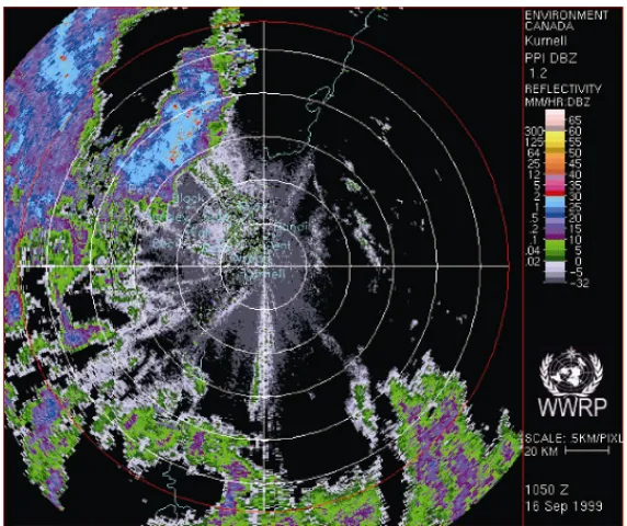
1.1 An Example of Doppler Radar Reflectivity Image(1999, September 16th,

10:50) provided by Dr. Paul Joe from Environment Canada . . . 3

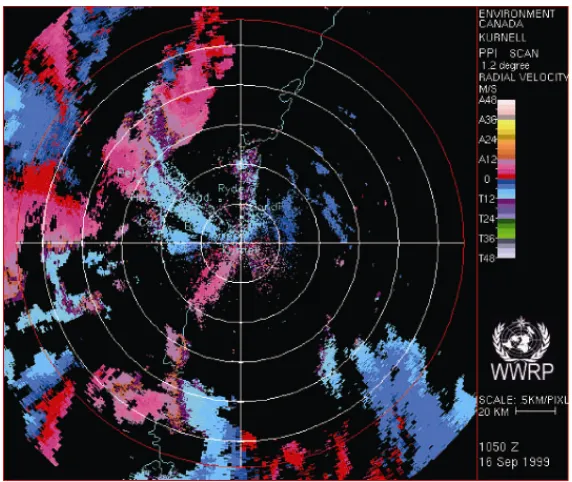
1.2 An Example of Doppler Radar Velocity Image(1999, September 16th_,

10:50) provided by Dr. Paul Joe from Environment Canada . . . 4

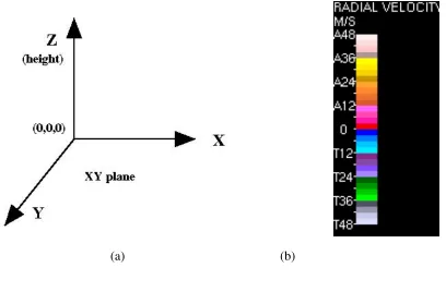
1.3 (a) The coordinate system used by 3D velocity representation and (b) the

colour-magnitude correspondence map used for Doppler radial velocity. . . 5

1.4 The structure of NEXRADI Doppler radar dataset. The NEXRADII data is

structured in a similar way. . . 6

1.5 The Doppler and windprofiler radars in southwestern Ontario and the

ad-jacent Northern American area states (the Great Lakes area). The Doppler

radars at Detroit, Cleveland and Buffalo are shown as red dots, the Doppler

radars at King City and Exeter are shown as blue dots and the windprofiler

radars are at Harrow and Washingham are shown as orange dots. . . 10

2.1 Retrieved full velocity by least squares method on radar data (2000, August

28th, 01:02) . . . 26

2.2 Retrieved full velocity by Regularization method on radar data (2000,

Au-gust 28th_{, 01:02) . . . 26}

2.3 Cartesian Coordinate System, cited from Armijo’s paper [1] . . . 27

2.4 Coplanar Cylindrical Coordinate System, from Testud and Chong [71] . . . 28

2.5 Antenna beam configuration for the 5-beam UHF wind profiler, from

Strauchet al.[67]. . . 34

(13)

4.1 3D full Velocity Flow using single Least Squares methods on real data at

13:59:12 of August 20th_{, 2007 at Detroit and at 14:00:30 of August 20}th_,

2007 at Cleveland. (a) theUV flow, (b) theU component, (c) the V

com-ponent and (d) theW component. . . 74

4.2 3D full Velocity Flow using dual Least Squares methods on real data at

4.3 3D full Velocity Flow using single Regularization methods on real data at

4.4 3D full Velocity Flow using dual Regularization methods on real data at

5.1 An example of coloured Doppler radial velocity data (from elevation 0,

August 19th_{, 2007 Detroit Doppler data) with the location of the Harrow}

wind profiler and its area of influence indicated. . . 81

(14)

flow, (b) theU component of the unrefined optical flow, (c) theV

compo-nent of the unrefined optical flow, (d) theW component of the unrefined

optical flow and (e) the refinedUV optical flow, (f) theU component of the

refined optical flow, (g) theVcomponent of the refined optical flow, (h) the

Wcomponent of the refined optical flow. . . 84

5.3 Error results of the synthetic data for allK values: (a) the average output

error, (b) the average magnitude error, (c) the average direction error, (d)

the average xangular error, (e) the averageyangular error and (f) the

aver-agezangular error. The blue lines show the performance of the unrefined

retrieval, the red lines show the performance of the refined method with

0% input windprofiler error and the green lines show the performance of

the refined method with 10% windprofiler input error. . . 86

5.4 The correct synthetic velocity at variation level K = 5: (a) the correct

UV flow as a vector field on coloured radial velocity, (b) the correct U

component, (c) the correctV component and (d) the correctW component.

The retrieved synthetic velocity at variation levelK = 5: (e) the unrefined

UV optical flow, (f) the unrefinedU component of optical flow along thex

axis, (g) the unrefinedV optical flow along theyaxis, (h) the unrefinedW

component of optical flow along thezaxis, and (i) the refined UV optical

flow, (j) the refinedU component of optical flow along the xaxis, (k) the

refined V optical flow along the Y axis, (l) the refined W component of

optical flow along thezaxis. . . 88

5.5 Average output error for (a)Γ = 1000 and for (b)Γ = 1800, both with for

σ3 = 0.4 (diamond curves), 0.7 (square curves) and 1.0 (triangle curves)

for the synthetic velocity for the variousKvalues. . . 90

(15)

3 = 3= 3= 3=

5.7 The refinedU velocity component along thexaxis of the synthetic velocity

forK = 5 with variousσ3,Γvalues: (a)σ3 = 0.4, Γ =1000, (b)σ3 =0.4,

Γ =1800, (c)σ3 = 1.0,Γ =1000 and (d)σ3= 1.0,Γ =1800. . . 91

5.8 The horizontal velocity retrieved from Detroit Doppler (and the radiosonde

experiment) data on June 28th_{, 2007 at 00:18:42 for elevation 1: (a) the}

unrefined UV optical flow, (b) the U component of the unrefined optical

flow, (c) theV component of the unrefined optical flow, and (d) the refined

UVoptical flow, (e) theUcomponent of the refined optical flow and (f) the

V component of the refined optical flow. . . 93

5.9 The horizontal velocity retrieved from Detroit Doppler (and the radiosonde

experiment) data on June 28th, 2007 at 00:18:42 for elevation 2: (a) the

unrefined UV optical flow, (b) the U component of the unrefined optical

flow, (c) theV component of the unrefined optical flow, and (d) the refined

UVoptical flow, (e) theUcomponent of the refined optical flow and (f) the

V component of the refined optical flow. . . 94

7.1 (a) Artificial tracking result using original storm tracking tracking

algo-rithm; (b) Artificial tracking result using pseudo storms and the original

storm tracking algorithm; (c) Artificial tracking result using pseudo storm

and a connection between a pseudo storm and a real storm. . . 125

7.2 Artificial tracking results for a more complicated case: (a) using the original

tracking algorithm; (b) using the original tracking algorithm with pseudo

storms; (c) using pseudo storm and our new pseudo storm tracking

algo-rithm. . . 128

7.3 (a) The organization of a typical adjacency with pseudo storms; (b)

ing an adjacency where the real storms have multiple disparities; (c)

Build-ing an adjacency in a more complicated situation. . . 129

(16)

A.1 The correct synthetic velocity of group 1 at variation level K = 0: (a) the

correctUVflow, (b) the correctU component, (c) the correctV component

and (d) the correctW component. . . 155

A.2 The single retrieved synthetic velocity of group 1 at variation level K = 0

and noise levelL = 4: (a) the retrieved UV flow, (b) the retrievedU

com-ponent, (c) the retrievedV component and (d) the retrievedW component. . 156

A.3 The dual retrieved synthetic velocity of group 1 at variation levelK = 0 and

noise levelL=4: (a) the retrievedUVflow, (b) the retrievedUcomponent,

(c) the retrievedV component and (d) the retrievedWcomponent. . . 157

A.7 Result Analysis of Synthetic Data Group 1: (20.0, 20.0, 20.0). The Single

Retrieval (a), (c), (e) and Dual Retrieval (b), (d), (f). . . 161

Retrieval (g), (i), (k) and Dual retrieval (h), (j), (l). . . 162

(17)

(18)

(19)

(20)

B.1 The correct synthetic velocity of group 1 at variation level K = 0: (a) the

(21)

= =

retrievedUcomponent, (c) the retrievedVcomponent and (d) the retrieved

Wcomponent. . . 205

B.3 The dual regularization retrieved synthetic velocity of group 1 at variation

level K = 0 and noise level L = 4: (a) the retrieved UV flow, (b) the

Wcomponent. . . 206

B.5 The single regularization retrieved synthetic velocity of group 1 at variation

Wcomponent. . . 208

Wcomponent. . . 209

B.7 Result Analysis of Synthetic Data Group 1 using regularization method:

(20.0, 20.0, 20.0). The Single Retrieval (a), (c), (e) and Dual Retrieval (b),

(d), (f). . . 210

(20.0, 20.0, 20.0). The Single Retrieval (g), (i), (k) and Dual retrieval (h),

(j), (l). . . 211

(22)

= =

Wcomponent. . . 213

Wcomponent. . . 214

Wcomponent. . . 216

Wcomponent. . . 217

(d), (f). . . 218

(j), (l). . . 219

(23)

= =

Wcomponent. . . 221

Wcomponent. . . 222

Wcomponent. . . 224

Wcomponent. . . 225

(5.0, 5.0, 5.0). The Single Retrieval (a), (c), (e) and Dual Retrieval (b), (d),

(f). . . 226

(5.0, 5.0, 5.0). The Single Retrieval (g), (i), (k) and Dual retrieval (h), (j), (l). 227

(24)

= =

Wcomponent. . . 229

Wcomponent. . . 230

Wcomponent. . . 232

Wcomponent. . . 233

(20.0, 20.0, 5.0).The Single Retrieval (a), (c), (e) and Dual Retrieval (b),

(d), (f). . . 234

(j), (l). . . 235

(25)

= =

Wcomponent. . . 237

Wcomponent. . . 238

Wcomponent. . . 240

Wcomponent. . . 241

(d), (f). . . 242

(j), (l). . . 243

(26)

= =

Wcomponent. . . 245

Wcomponent. . . 246

Wcomponent. . . 248

Wcomponent. . . 249

(d), (f). . . 250

(j), (l). . . 251

D.1 The tracks on Images (aa) and (ab) of the 27 images using the original

relaxation labeling algorithm from the Detroit/Cleveland Doppler data on

August 20th_{, 2007 . . . 259}

(27)

/

August 20th, 2007 . . . 260

D.1 The tracks on Images (ae) and (a f) of the 27 images using the original

August 20th_{, 2007 . . . 261}

D.1 The tracks on Images (ag) and (ah) of the 27 images using the original

August 20th, 2007 . . . 262

D.1 The tracks on Images (ai) and (a j) of the 27 images using the original

August 20th_{, 2007 . . . 263}

D.1 The tracks on Images (ak) and (al) of the 27 images using the original

August 20th_{, 2007 . . . 264}

D.1 The tracks on Images (am) and (an) of the 27 images using the original

August 20th, 2007 . . . 265

D.1 The tracks on Images (ao) and (ap) of the 27 images using the original

August 20th_{, 2007 . . . 266}

D.1 The tracks on Images (aq) and (ar) of the 27 images using the original

August 20th, 2007 . . . 267

D.1 The tracks on Images (as) and (at) of the 27 images using the original

August 20th_{, 2007 . . . 268}

(28)

/

August 20th, 2007 . . . 269

D.1 The tracks on Images (aw) and (ax) of the 27 images using the original

August 20th_{, 2007 . . . 270}

D.1 The tracks on Images (ay) and (az) of the 27 images using the original

August 20th, 2007 . . . 271

D.1 The tracks on Image (ba) of the 27 images using the original relaxation

labeling algorithm from the Detroit/Cleveland Doppler data on August 20th_,

2007 . . . 272

D.2 The tracks on Images (aa) and (ab) of the 27 images with pseudo storms

using the original relaxation labeling algorithm from the Detroit/Cleveland

Doppler data on August 20th_{, 2007 . . . 273}

D.2 The tracks on Images (ac) and (ad) of the 27 images with pseudo storms

Doppler data on August 20th, 2007 . . . 274

D.2 The tracks on Images (ae) and (a f) of the 27 images with pseudo storms

D.2 The tracks on Images (ag) and (ah) of the 27 images with pseudo storms

D.2 The tracks on Images (ai) and (a j) of the 27 images with pseudo storms

(29)

/

D.2 The tracks on Images (am) and (an) of the 27 images with pseudo storms

D.2 The tracks on Images (ao) and (ap) of the 27 images with pseudo storms

D.2 The tracks on Images (aq) and (ar) of the 27 images with pseudo storms

D.2 The tracks on Images (as) and (at) of the 27 images with pseudo storms

D.2 The tracks on Images (au) and (av) of the 27 images with pseudo storms

D.2 The tracks on Images (aw) and (ax) of the 27 images with pseudo storms

D.2 The tracks on Images (ay) and (az) of the 27 images with pseudo storms

D.2 The tracks on Image (ba) of the 27 images with pseudo storms using the

original relaxation labeling algorithm from the Detroit/Cleveland Doppler

data on August 20th_{, 2007 . . . 286}

(30)

/

D.3 The tracks on Images (ac) and (ad) of the 27 images with pseudo storms

using the pseudo relaxation labeling algorithm from the Detroit/Cleveland

D.3 The tracks on Images (ae) and (a f) of the 27 images with pseudo storms

D.3 The tracks on Images (ag) and (ah) of the 27 images with pseudo storms

D.3 The tracks on Images (ai) and (a j) of the 27 images with pseudo storms

D.3 The tracks on Images (ak) and (al) of the 27 images with pseudo storms

D.3 The tracks on Images (am) and (an) of the 27 images with pseudo storms

D.3 The tracks on Images (ao) and (ap) of the 27 images with pseudo storms

D.3 The tracks on Images (aq) and (ar) of the 27 images with pseudo storms

(31)

/

D.3 The tracks on Images (au) and (av) of the 27 images with pseudo storms

D.3 The tracks on Images (aw) and (ax) of the 27 images with pseudo storms

D.3 The tracks on Images (ay) and (az) of the 27 images with pseudo storms

D.3 The tracks on Image (ba) of the 27 images with pseudo storms using the

pseudo relaxation labeling algorithm from the Detroit/Cleveland Doppler

data on August 20th_{, 2007 . . . 300}

E.1 The tracks on Images (aa), (ab), (ac), (ad), (ae) and (a f) of the 64 images

using original relaxation labeling algorithm from the Detroit/Cleveland

E.2 The tracks on Images (ag), (ah), (ai), (a j), (ak) and (al) of the 64 images

E.3 The tracks on Images (am), (an), (ao), (ap), (aq) and (ar) of the 64 images

E.4 The tracks on Images (as), (at), (au), (av), (aw) and (ax) of the 64 images

(32)

/

E.6 The tracks on Images (be), (b f), (bg), (bh), (bi) and (b j) of the 64 images

E.7 The tracks on Images (bk), (bl), (bm), (bn), (bo) and (bp) of the 64 images

E.8 The tracks on Images (bq), (br), (bs), (bt), (bu) and (bv) of the 64 images

E.9 The tracks on Images (bw), (bx), (by), (bz), (ca) and (cb) of the 64 images

E.10 The tracks on Images (cc), (cd), (ce), (c f), (cg) and (ch) of the 64 images

E.11 The tracks on Images (ci), (c j), (ck) and (cl) of the 64 images using original

August 19th_{, 2007 . . . 312}

E.12 The tracks on Images (aa), (ab), (ac), (ad), (ae) and (a f) of the 64

im-ages using advanced pseudo storm relaxation labeling algorithm from the

Detroit/Cleveland Doppler data on August 19th, 2007 . . . 313

E.13 The tracks on Images (ag), (ah), (ai), (a j), (ak) and (al) of the 64 images

using advanced pseudo storm relaxation labeling algorithm from the

De-troit/Cleveland Doppler data on August 19th_{, 2007 . . . 314}

(33)

E.15 The tracks on Images (as), (at), (au), (av), (aw) and (ax) of the 64

Detroit/Cleveland Doppler data on August 19th_{, 2007 . . . 316}

E.16 The tracks on Images (ay), (az), (ba), (bb), (bc) and (bd) of the 64

E.17 The tracks on Images (be), (b f), (bg), (bh), (bi) and (b j) of the 64

Detroit/Cleveland Doppler data on August 19th_{, 2007 . . . 318}

E.18 The tracks on Images (bk), (bl), (bm), (bn), (bo) and (bp) of the 64

E.19 The tracks on Images (bq), (br), (bs), (bt), (bu) and (bv) of the 64 images

E.20 The tracks on Images (bw), (bx), (by), (bz), (ca) and (cb) of the 64

E.21 The tracks on Images (cc), (cd), (ce), (c f), (cg) and (ch) of the 64 images

E.22 The tracks on Images (ci), (c j), (ck) and (cl) of the 64 images

us-ing advanced pseudo storm relaxation labelus-ing algorithm from the

(34)

1.1 The elevation angles (angles of the cone walls with the positivezaxis) of

NEXRADIand NEXRADIIDoppler radars . . . 7

4.1 The values of parameters chosen for 3D full velocity retrieval experiments

using dual least squares and regularization methods. . . 63

(35)

Introduction

In meteorology, severe weather storms refer in part to the localized convection caused by

updrafts and downdraughts in the air. Usually severe storms focus on a smaller area

com-pared to tropical cyclone areas, with a duration varying from about half an hour to a couple

of hours. Severe storms can be classified into single-cell, multi-cell or super-cell storms,

according to their scale. They could produce violent weather phenomena in the form of

thunderstorms, hail, heavy rains, or even tornadoes with heavy precipitation. Severe storms

are the most common natural hazards and can cause significant critical lost of life and

prop-erty damage. Therefore, an important task for meteorologists is to forecast the formation of

severe storms. This task includes the detection of severe storms, the measurement of their

sizes and motion and the tracking of storms through their life cycles.

1.1 Doppler Radar

Doppler radar has been considered to be a valuable observation tool in meteorology for a

long time [59]. It is capable of observing high resolution information about the internal

structure of severe weather storms hundreds of kilometers from the radar. In 1842,

Chris-tian Doppler [23] observed that sound waves would have a higher frequency if the source

was moving toward the observer and a lower frequency if the source was moving away

(36)

from the observer. This phenomenon not only applies to sound waves, but to all types of

waves. If one measures how long it takes for a ordinary radar wave to reflect back from an

environmental particle (say a rain drop) to the radar then one can use that time to calculate

how far the particle is from the radar. The frequency it detects from a moving object can

be calculated as in Equation 1.1:

fDoppler= 2∗Vtarget

ftransmitted

c , (1.1)

whereVtarget is the velocity of the object according to the radar, ftransmitted is the frequency

originally transmitted from the radar andcis the velocity of light.

With a Doppler radar, one can not only compute whether a raindrop is moving toward

or away from the radar but the speed of the rain drop as well (along the line from the radar

to the rain drop). This calculation is based on the rate of compression or expansion of the

radar wave, i.e. the Doppler effect. The speed and radial direction together comprise the

radial velocity. Since wind causes rain drops to move, this radial velocity is actually a type

of wind velocity measurement. Precipitation density (reflectivity) relates to the amount of

the rain in a unit volume and is measured by the strength of the reflected wave.

Figure 1.1 depicts the reflectivity image detected by Doppler radar in Sept. 16th _1999,

10:50. The different colours in the image represent the different densities of reflectivity,

according to the colour map. As the colour changes, the magnitude of reflectivity could be

up to 65 dBZ (decibels of Z). If the reflectivity is > 65 dBZ the rain is extremely heavy,

between 46−65 dBZ it is heavy, between 24−45 dBZ it is moderate, between 8−23 it is

light and between 0−8 dBZ there is barely any rain at all1_.

The actual reflectivity values detected by radar are at discrete voxel locations. Fig 1.1

is the result of a bilinear patch algorithm [56] that was used to smooth/fill in this voxel

data. Without bilinear interpolation the image would looks like a sparse collection of rays

transmitting from the radar center. Later we will see the recognition and tracking of severe

storms are all based on this reflectivity image [4, 5, 17, 56, 57, 68, 69, 70].

(37)

Figure 1.1: An Example of Doppler Radar Reflectivity Image(1999, September 16th_{, 10:50)}

provided by Dr. Paul Joe from Environment Canada

Figure 1.2 shows the radial velocity image automatically generated by radar. It was

acquired at the same time as the reflectivity image in Figure 1.1. The coloured parts cover

a similar area as in the reflectivity case, demonstrating the wind movements over that area.

The different colours here represent not only the magnitudes but also their directions, as

shown in the colour map. Basically, “Red” represents a positive direction, which means the

wind is moving away from the radar, while “Blue” implies a negative wind velocity, which

is moving towards the radar. It must be noted that the velocity detected by radar is only

the radial parts (i.e. in the direction of transmitting beams). Earlier work has shown how

to utilize this knowledge to retrieve an approximation to the full 3D velocity of wind field

[6, 13, 14, 15].

The coordinate system used in the 3D velocity representation is shown in Figure 1.3a.

Thexaxis is left to right, theyaxis is from bottom to top and thezaxis is height (upwards).

(38)

Figure 1.2: An Example of Doppler Radar Velocity Image(1999, September 16th_{, 10:50)}

provided by Dr. Paul Joe from Environment Canada

Figure 1.4 illustrates the 3D structure of NEXRADI (Next-GenerationRadar Level I)

Doppler radar data. The radar data covers approximately a circular cone, with area roughly

about 87,000 km2. There are 15 elevations of data with the cone angle centered at the

radar location, changing from the minimum angleΦminof 58◦to a maximum angleφmaxof

89.5◦. The length of cone radii varies from a minimum 508.84kmto an maximum radius of

599.97km. Vertically the height of elevation is from the ground level, 5.25km, up to 317.4

km. At each elevation, there are 360 beams transmitting (one beam per degree of a circle).

For each degree of the beam, there are 600 points where reflectivity/radial velocity data

is measured. These points are referred to as voxels because they represent the integration

of such data in 3D frustums at those points. Table 1.1 shows more details about the angle

(measured according to the vertical axis). All previous research uses this type of radar data

[4, 5, 17, 56, 57, 68, 69, 70].

(39)

(a) (b)

Figure 1.3: (a) The coordinate system used by 3D velocity representation and (b) the

colour-magnitude correspondence map used for Doppler radial velocity.

has placed several Doppler radars around the Great lakes area. They are using the next

generation of NEXRAD radar data called NEXRAD II. The NEXRAD II datasets share

a similar structure with the NEXRAD I. However, its data structure is capable of storing

dynamic parameters, so that the number of elevations and resolution of the radar beams can

change. Generally, a NEXRAD II radar has fewer elevation numbers than a NEXRAD I

radar, about only 9 elevations down from 15 before (Usually the higher elevations contain

fewer data so they are not that useful). There are 920 voxels to record reflectivity data,

covering a circular area with radius of 460 kmat each elevation. So the coverage area of

reflectivity data is smaller but the resolution along each beam is twice as high as before.

There are 920 voxels to record radial velocity data, but the radius of the coverage circle

is only 230 km. Thus the radial velocity data covers a much smaller area (half of the

reflectivity data area and about a quarter of NEXRAD I data area) with a resolution of

(40)

velocity vector since there is only smaller variation of the data in this dimension. Table

1.1 shows the elevation angles for the NEXRAD II data. It can be seen that the overall

number of angles for the NEXRAD II data are smaller than the NEXRAD I angles. The

NEXRAD II data focuses more on the lower height area than NEXRAD I, where the W

velocity component is almost orthogonal to the radial velocities. So radial velocity contains

little reliable W information (and is extremely sensitive to noise). This is an example of

the Aperture Problem [3], where most of the local velocity information is orthogonal to

underlying 3D velocity. We will show how to overcome or attenuate this problem using

algorithms presented in this thesis.

Figure 1.4: The structure of NEXRADI Doppler radar dataset. The NEXRADII data is

structured in a similar way.

1.2 Our Problems

In order to understand how storms develop and move over time, much research has been

devoted to retrieving 3D full wind velocity from the observed radial velocity (for example,

(41)

Elevation Number NEXRADI Angle (φ◦₎ _NEXRAD_II_{Angle (}φ◦₎

0 89.5 89.5

1 88.8 88.51

2 88.1 87.5

3 87.3 86.57

4 86.5 85.65

5 85.3 83.94

6 84.0 80.07

7 82.5 75.37

8 80.8 70.44

9 79.0 NA

10 77.0 NA

11 74.0 NA

12 70.0 NA

13 65.0 NA

14 58.0 NA

Table 1.1: The elevation angles (angles of the cone walls with the positive z axis) of

NEXRADI and NEXRADIIDoppler radars

than using the traditional methods provided by meteorologists (see Chapter 2), we solve

this problem using the 3D Optical Flow framework ([14, 15, 69]), which is a technology

widely applied in the Computer Vision area. 2D optical flow estimates the 2D image motion

of pixels in an image taken from an image sequence. The 3D extension of 2D optical flow

allows the computation of the 3D volumetric motion of voxels in a sequence of 3D volumes.

In meteorology applications, 3D optical flow is a measure of 3D wind velocity. Reliable

performance has been obtained on real 3D Doppler radar data (NEXRADI) [14, 15] using

(42)

We used 3D optical flow to recover full 3D wind velocity from radar data measured

by NCDC Doppler radars in the Great Lakes area. However, previous optical flow work

[4, 5, 17, 56, 57, 68, 69, 70] used only one Doppler radar. In the Great Lakes region,

the coverage areas of the radars often overlap and this suggests the possibility to combine

them. This thesis shows how to use multiple Doppler radars in both the Least Squares

and the Regularization frameworks to enhance the performance. We call the advanced

least squares method the Dual LS(Least Squares) approach as opposed to the original

Single LS approach proposed before [14], and refer to our refined regularization method

as the Dual Regularization approach as opposed to the original Single Regularization

approach proposed before [15]. In addition to qualitatively evaluating the optical flow

results for the real Great Lakes radar datasets, we also quantitatively examine the optical

flow performance using various synthetic Doppler radar datasets.

Recently, another type of Doppler radar, the Ontario-Quebec VHF Windprofiler Radar

Network (O-Q net) has also been installed around the same Great Lakes area. These radars

are also Doppler radars, but compared to the traditional precipitation-based Doppler radars

as we previously discussed, they cover a relatively smaller area and do not have the

lim-itations in the upward direction for wind velocity retrieval. The windprofiler radar uses

radio waves to detect the wind speed and direction at various elevations above the ground

and work even when little or no precipitation is not present. It is believed that

windprofil-ier radars can provide accurate local wind measurements up to 15 km high. Therefore in

this thesis, we consider how to integrate the data from windprofiler to precipitation-based

Doppler radar, which allows more accurate wind measurements in the overlapping radar

areas, especially in the upwards direction (where Doppler radar wind recovery is weak).

We present another modification to the regularization method used above, which we call

the “refined” regularization approach, to integrate windprofiler and Doppler data. Again,

we qualitatively evaluate our flow on real Great Lakes windprofiler and Doppler datasets

and quantitatively on synthetic windprofiler and Doppler datasets.

(43)

investigate storm tracking using the reflectivity data provided by Doppler radar (3D velocity

is one compatibility function in our tracking algorithm). Based on previous work [56, 68,

69, 70] we propose a new storm detection and tracking algorithm that builds on previous

work and is capable of working in a multiple-Doppler radar environment. To handle the

complicated storm patterns resulting from using multiple overlapping radars, we expand

on a novel concept called “Pseudo Storms”. This idea was initially introduced by Krezeski

et al. [41] for 2D storm tracking. In addition to 3D pseudo storm, we present a tracking

algorithm that uses this concept to track storms that not only change their shapes and sizes

over time but also merge with other storms to a bigger storm or split into a number of

smaller storms. Krezeski et al. did not present a pseudo storm tracking algorithm [41]. A

comparison between the original tracking algorithm (see [5, 17, 70]) and the new pseudo

tracking algorithm is given.

Figure 1.5 shows the distribution of Doppler radars and other radars such as

windprofil-ers around the lower Great Lakes area in North America, especially around Lake Erie. We

have acquired NEXRADII data from the Detroit and Cleveland radars via the NCDC

(Na-tional Climate Data Center) network in the US. We have also acquired Canadian Doppler

radar data from the King City and Exeter radars.

1.3 Thesis Contributions

We briefly enumerate the contributions of this thesis:

1. We propose a generalized framework to compute 3D optical flow in order to recover

the 3D full wind velocity via multiple Doppler radars.

2. We have integrated windprofiler radar data into our framework, to enhance the

accu-racy of wind velocity recovery, especially in the upward direction.

3. Experiments using both real data and synthetic data are used to qualitatively and

(44)

Figure 1.5: The Doppler and windprofiler radars in southwestern Ontario and the

adja-cent Northern American area states (the Great Lakes area). The Doppler radars at Detroit,

Cleveland and Buffalo are shown as red dots, the Doppler radars at King City and Exeter

are shown as blue dots and the windprofiler radars are at Harrow and Washingham are

shown as orange dots.

4. We introduce the pseudo storm idea as a better representation of the continually

de-forming real storms. We have redesigned the original tracking algorithm to

imple-ment pseudo storm into it.

5. We propose an advanced storm tracking algorithm using pseudo storm with its full

advantages. This new pseudo storm tracking solution can generate reasonable results

in a more comprehensive situation, compared to the original tracking algorithm.

1.4 Overview of Thesis

Chapter 2 presents a literature survey of the previous work on 3D wind recovery from

(45)

using multiple (dual) Doppler radars and finally using windprofiler radars. The second part

of the literature survey deals with storm detection and tracking in Doppler radar datasets.

After the literature survey, the thesis is divided into two parts. In PART I, we

concen-trate on the recovery of full 3D wind velocity using optical flow methods from single and

multiple Doppler and/or windprofiler radars. In PART II, we show how to detect and track

severe storm in Doppler radar datasets. Chapters 3, 4, 5 belong to PART I. Chapters 6, 7

belong to PART II.

Chapter 3 presents the modified least squares and regularization methods used to

re-cover 3D wind velocity using single or multiple Doppler radar datasets.

Chapter 4 presents the design and quantitative analysis of our synthetic Doppler radar

datasets. The results for the Great Lakes real Doppler radar datasets are also presented.

Chapter 5 shows the integration of windprofiler radar data into our optical flow solution,

adding extra information on the upward direction of 3D wind velocity to our optical flow

algorithms. We quantitatively and qualitatively evaluate our algorithm on synthetic and real

Doppler and windprofiler datasets.

Chapter 6 presents the storm detection algorithm in Doppler radar datasets and the data

structures necessary to represent them. To solve the limitations of the original method, we

introduce a “pseudo storm” idea. We also modify the original tracking algorithm to use a

restricted pseudo storms definition in our program, which shows advantages but still has its

limitations.

Chapter 7 presents the advanced storm tracking algorithm using pseudo storms

thor-oughly to generate better tracks than both the original tracking algorithm and the modified

one (that only has restricted pseudo storms implemented). Results from all the algorithms

are displayed and compared.

(46)

Literature Survey

The original data obtained from precipitation-based Doppler radar comprise:

1. the reflectivity or precipitation density,

2. the radial component of full wind velocity in the direction of radar beam and

3. the spectrum width (effectively the spectral and temporal variance in the local radial

velocities).

Reflectivity and radial velocities are used for full velocity retrieval and storm tracking,

while the spectrum width (effectively, the variance of the radial velocities within a voxel)

can help estimate the reliability of radial velocity. We use a spectrum width threshold of 30

dBZ to identify unreliable radial velocities in this thesis.

To better understand the motion of wind in the atmosphere (and, hence, the motion of

severe storms as they move with the wind), meteorologists need more detailed 3D

informa-tion, such as the 3D wind velocity field. Since the very beginning of radar application for

severe storm nowcasting/forecasting, much research has been devoted to the use of Doppler

radar. The initial application in the early days can be found in R. J. Doviak and D. S. Zrni´c’s

book [25]. Computer Vision techniques allow radar data to be treated as images of storm

motion and deformation. By analyzing the attributes of these images, more detailed and

(47)

accurate views of 3D wind motion can be obtained. Based on this information, a more

reliable prediction of severe storms behavior can be predicted.

2.1 Retrieving 3D Velocity by Single Doppler Radar

A significant amount of research has been devoted to the retrieval of 3D full wind velocity.

Since the Doppler radar can only measure the radial wind velocity, additional constraints

must be employed to recover 3D velocity. In order to do that, one hypothesis made was

that there is only very little modification of wind field when it moves across the radar’s

view range [45]. As well, all the data in a radar’s data volume is assumed to be detected

simultaneously (actually there is a significant time difference between the times the first

and last data items are measured due to the radar rotating 360◦ for each elevation of data

acquired). In the following sections below we present traditional approaches to the recovery

of 3D full wind velocities using data from a single Doppler radar. We also discuss the use

of optical flow techniques from the Computer Vision area to measure 3D wind velocity (we

use the wordsvelocityandflowinterchangeably). The traditional approaches try to fit the

observed radial velocities into various models while the optical flow approach uses various

constraint of 3D motion, which are not directly derived from the physics of wind motion.

2.1.1 Traditional Approaches to Retrieve 3D Wind Velocity

In order to simplify the retrieval process in the single Doppler radar case, usually an

as-sumption is made that wind properties changes linearly. Lhermitte and Atlas [45]

pro-posed the VAD (Velocity Azimuth Display) approach to estimate the mean horizontal wind

magnitude (in the 2D plane) and the direction about horizontal circles centered about the

vertical axis of radar. It was shown that some parameters of the wind velocity, such as the

mean convergence, divergence and deformation, could also be retrieved by this method.

Furthermore, Easterbrook [27] proposed that this retrieval could also be performed in a

(48)

reli-able results with the lower elevations in the clean air case. Later, Waldteufel and Corbin

[72] extended VAD and VARD into a more sophisticated technique, the VVP (Volume

Ve-locity Processing) technique, which processes radar data in a volume. This solution is the

most advanced one among all the traditional solutions.

2.1.1.1 The VAD Analysis Procedure

For any given environmental point (x0,y0,z0), the linearity assumption for wind fieldV~ =

(u,v,w) can be expressed as:

u=u0+u0x(x−x0)+u 0

y(y−y0)+u 0

z(z−z0)

v=v0+v0x(x−x0)+v 0

y(y−y0)+v 0

z(z−z0) (2.1)

w=w0+w0x(x−x0)+w 0

y(y−y0)+w 0

z(z−z0)

whereV~ = (u,v,w) is the 3D wind velocity that varies linearly around its value (u0,v0,w0)

at a point (x0,y0,z0). Theu0and so on are the derivatives of velocity components on the x,

y,zaxes.

At the same time, the magnitude of the radial velocity can be estimated in Polar

coor-dinates as:

Vr = ucosθcosφ+vsinθcosφ+wsinφ (2.2)

whereθis the azimuth angle whileφis the elevation angle. Combing these two equations