Volume 7, No. 3, May-June 2016
International Journal of Advanced Research in Computer Science RESEARCH PAPER
Available Online at www.ijarcs.info
Missed Deadlines Should be Considered- Proposals for Modifying Existing Real-Time
Disk Scheduling Algorithms
Wamika Basu
Department of Computer Science and Engineering Birla Institute of Technology, Mesra, Kolkata Campus
Kolkata, India
Subho Chaudhuri
Department of Computer Science and Engineering Birla Institute of Technology, Mesra, Kolkata Campus
Kolkata, India
Abstract: A system is said to be a real time system if it is capable of producing the correct results within a particular time limit. This time limit is called deadline. Real time systems may be hard or soft. A hard real time system may be considered to have failed if it is unable to produce the correct results within its allotted time span. Examples of hard real time systems are pacemakers, anti-lock brakes and aircraft control systems. In soft real time systems, deadline misses are tolerable, but may degrade the system’s quality of service. Scheduling is the basic mechanism adopted by a real time system to meet the deadline. Hence, scheduling algorithms dictate the proper functioning of real time systems. This paper aims to propose modifications to the existing real time disk scheduling algorithms. The modifications were made to include tardiness while assigning priorities to the disk requests. The modified algorithms were then experimentally compared with the existing ones on several parameters like seek time, average waiting time and average turnaround time.
Keywords: Deadline; hard and soft real time systems; disk scheduling; tardiness; seek time; average waiting time; average turnaround time.
I. INTRODUCTION
Tardiness measures how late a job completes with respect to its deadline. If the job completes at or before its deadline, then the tardiness is zero. On the other hand, if the job completes after its deadline, then tardiness is equal to the difference between its completion time and its deadline. In real time disk scheduling, tardiness measures how late a disk request is serviced with respect to its deadline. In soft real time systems, the usefulness of a result produced after its deadline is not zero. The usefulness degrades as time passes after the deadline. Hence, the usefulness of a result produced after its deadline decreases as the tardiness increases. This implies that a process (in this case disk read/write) is still useful when the soft deadline is crossed. This concept is at the core of our proposed algorithms. As the number of disk read/write requests will tend to become larger and larger- specially with respect to growing number of disk servers (web servers, video-on-demand servers, transaction servers etc), disk farms etc, and also with respect to increasing number of processes and threads, the number of disk requests missing their deadlines will continue to increase. So in our view, tardiness could be an important parameter towards optimizing real time disk scheduling.
II. OVERVIEW OF DISK STRUCTURE
A. Physical Structure
A disk has several circular-shaped platters. Platters are made of metal or plastic and have a magnetisable coating on them. Each platter has two surfaces. Information is stored on the platters by recording it magnetically on them. Each surface has concentric set of magnetic paths. These paths are called tracks. The set of tracks across all surfaces at the same arm position is called a cylinder. Tracks are further subdivided into sectors. The data on a disk are read/written by read/write heads.
There is one head on each surface of the platter. The disk arm moves the heads together from one cylinder to the other.
Figure 1. Disk Structure[1]
B. Working Principle
The access time of a disk can be specified by random time and transfer time (as a function of information amount). In addition, there is the device queue time and channel wait time [2].
Random Time
This has two components: Seek Time and Rotational Latency.
Seek Time
In a movable-head disk, there is only one arm to service all the disk tracks. The time taken by the disk arm to move from one track to another where the data will be read or written is known as seek time. For performance evaluation, normally the average seek time is used.
Rotational Latency
the read/write head. The time spent in doing so is called rotational latency. For performance evaluation in general, average rotational latency is used, which is typically taken as 1/2x , where x is the rpm of the disk.
Transfer Time
This is the time required to transfer data to or from the disk. This is a function of the volume of the information and transfer speed of the disk to host connection bus.
Device Queue Time
This is the amount of time a disk request waits in the device queue for the device to be available if it is already allocated to another process.
Channel Wait Time
If a device shares a single I/O channel or a set of I/O channels with other disk drives, then the amount of time a disk request has to wait for the channel to be available is known as the channel wait time.
III. REAL-TIME DISK SCHEDULING
A. Disk Scheduling Problem
Disk subsystem is one of the slowest components of a computer system, and hence its performance is important for bettering the system throughput, more specifically in a real time environment. From this point of view, it is important to model the disk behavior as accurately as possible. The disk system uses a queue to maintain the outstanding disk requests. The disk relies on an appropriate scheduling algorithm for choosing which pending request in the queue should be processed next. Disk scheduling in real time systems is the process of ordering disk requests within the disk queue such that they are serviced within their deadlines with minimum mechanical motion of the disk arm by employing seek (and sometimes rotational latency) optimization techniques.
B. Existing Algorithms
In this section, we briefly describe five existing real time disk scheduling algorithms: EDF, SCAN-EDF, SSEDO, SSEDV and P-SCAN.
1) EDF: It is the most popular real time scheduling algorithm for both process and disk scheduling, and hence widely used. In EDF, the disk request with the earliest deadline has the highest priority and is serviced first. [3]
2) SCAN-EDF: SCAN-EDF is a combination of SCAN and EDF disk scheduling algorithms. It services requests with shorter deadlines first. In case of requests with same deadlines, it uses the SCAN approach. [4]
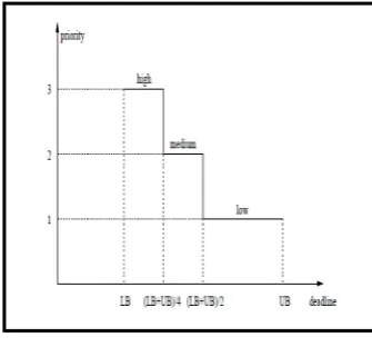
3) P-SCAN: The P-SCAN algorithm [5] divides disk requests into several priority levels (usually high, medium and low) according to their deadlines in the following way: if deadline of a request is bigger than (LB+UB)/2, then it is assigned a low priority. On the other hand, if the deadline of a request is less than (LB+UB)/4, then it is assigned a high priority. The request is assigned a medium priority if its deadline lies between (LB+UB)/4 and (LB+UB)/2. Here LB and UB are lower bound and upper bound of the relative deadlines respectively. Figure 2 shows the priority assignment of the P-SCAN algorithm as discussed above:
The SCAN algorithm is then used within each level. There is one queue for each priority level to maintain the outstanding disk requests at that level. The requests are arranged in increasing order of track positions within a queue. The scheduler always starts servicing the requests in the high priority queue with the smallest seek time. After this queue is exhausted, it schedules requests from medium priority queue, and in a similar fashion, with the exhaustion of requests, schedules from the low priority queue. The disadvantage of this algorithm is that if the number of priority levels is increased, then average seek time may worsen.
4) SSEDO: The shortest seek and earliest deadline by ordering algorithm (SSEDO) [6] uses a queue to store outstanding disk requests. Within the queue the requests are sorted based on their deadlines. An m size window is used to denote the first m requests with the smallest deadlines. Each request in the window is assigned a priority. Then the request with minimum priority value is chosen for service. The central idea behind this algorithm is to not only give highest priority to requests with earlier deadlines but to also allow a request with a longer deadline to get serviced if it is closer to the current disk arm position.
5) SSEDV: The shortest seek and earliest deadline by value algorithm (SSEDV) [6] is similar to the SSEDO algorithm in the sense that both are window algorithms. The only difference is that SSEDV uses the remaining lifetime of disk requests to assign priorities. Remaining lifetime of a request is the length of time between the current time and the deadline of the request.
C. Performance Analysis
In order to compare the performance of the algorithms mentioned in III B namely: EDF, SCAN-EDF, P-SCAN, SSEDO and SSEDV, a series of simulation experiments were conducted on them. In section 1, the simulation model for the experiments is described and the experimental results are given in section 2.
1) Simulation Model: In our model, the disk has 300 tracks. We have randomized the disk requests in terms of cylinder numbers ranging from 0-299. Each disk request has a deadline distributed randomly between 0 and 99 milliseconds. Disk service time is defined as the sum of seek time and rotational latency. Rotational latency is randomly distributed between 0 and 7 milliseconds. The read/write head is initially positioned at any random cylinder number in the range 0-299. The total number of disk requests (load to the system) ranges from 10 to 1000. For SSEDO, the window size m is taken as 3 and scheduling parameter β as 2. For SSEDV, the window size m is
three priority levels are considered- high, medium and low. Device Queue Time and Channel Wait Time are ignored.
2) Simulation Results: In this section, the experimental results are reported and carefully examined. The total seek time is plotted against the number of disk requests in Figure 3 below. The EDF algorithm performs fairly well when the system is lightly loaded but degenerates when the load increases. EDF results in excessive seek time as compared to the other algorithms. SCAN-EDF degenerates to EDF when all the requests have different deadlines. This is observed in the initial parts of the curve wherein SCAN-EDF results in the same seek time as EDF. As the number of requests increases, the probability of requests having similar deadlines increases. Hence SCAN-EDF optimizes the total seek time when the load increases as is evident from the latter part of the SCAN-EDF curve. SSEDO and SSEDV perform essentially at the same level, with the SSEDV algorithm performing better at high load cases. P-SCAN outperforms the other disk scheduling algorithms and optimizes the seek time to a great extent.
Figure 3. Seek Time vs Number of Disk Requests
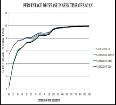
Figure 4 shows the percentage decrease in seek time of P-SCAN with respect to EDF, P-SCAN-EDF, SSEDO and SSEDV.
Figure 4. Percentage Decrease in Seek Time of P-SCAN
Some representative figures (as derived from the graph) with respect to percentage decline in seek times of P-SCAN over the other disk scheduling algorithms are stated in Table I:
Table I. Percentage Decrease in Seek Time of P-SCAN
Sr. No. A B C D E Legends in Table I:
A: Number of disk requests
B: % decrease in seek time of P-SCAN with respect to EDF C: % decrease in seek time of P-SCAN with respect to SCAN-EDF
D: % decrease in seek time of P-SCAN with respect to SSEDO
E: % decrease in seek time of P-SCAN with respect to SSEDV
Waiting time is defined as the amount of time a disk request waits in the disk queue before it is serviced. Figure 5 shows the average waiting time for 10-1000 disk requests. Here again, P-SCAN is optimal with respect to average waiting time.
Figure 5. Average Waiting Time vs Number of Disk Requests
Figure 6. Average Turnaround Time vs Number of Disk Requests
IV. PROPOSED ALGORITHMS
In this section, we propose two ways in which tardiness can be incorporated in the five real time disk scheduling algorithms mentioned above.
A. Basic idea of our Algorithms
None of the existing algorithms in section III B have taken tardiness into account, although we do have disk read/writes missing their deadlines (as revealed by our simulation study). We are proposing modifications to the existing real time disk scheduling algorithms by taking into account the tardiness of the requests.
1) Algorithm A
In our proposed algorithms named as: Modified EDF, Modified SCAN-EDF, Modified SSEDO, Modified SSEDV and Modified P-SCAN, we assume that the scheduler has knowledge of which disk requests are going to miss their deadlines. The scheduler will gain this knowledge by doing a virtual scheduling (as explained below) of the incoming disk requests by the existing scheduling algorithms- EDF, SCAN-EDF, SSEDO, SSEDV and P-SCAN one by one.
The basic idea of virtual scheduling is that the requests are ordered as dictated by the corresponding scheduling method (one of EDF, SCAN-EDF, SSEDO, SSEDV and P-SCAN). From that ordering, calculations are obtained as to the individual seek times- the seek times which require crossing the given deadlines indicate the fact that for those requests, the deadline will be missed. We make a note of all such requests which miss their deadlines. This implies they have tardiness incorporated in their completion.
After virtual scheduling, the scheduler will partition the requests into two distinct sets. One set will consist of the requests that will be serviced with given priorities (as defined for the corresponding scheduling policy) within their deadlines. The other set will include the requests that would be serviced after their deadlines.
For requests in the second set, priority is assigned in the following way:
a) Let Pi be the new priority of the ith request and Di be its deadline.
Then: Piα 1/Di
This implies that requests having shorter original deadlines are given higher priority for scheduling considerations with respect to the period past the deadline.
Then: Piα 1/Ti
This implies that requests having lower tardiness are also given higher priority for scheduling considerations with respect to the period past the deadline.
c) Considering a and b, we have: Piα 1/DiTi
or, Pi = K.1/DiTi, where K is the constant of proportionality
For simulation purpose K is taken as 1000 because of very small values of 1/DiTi.
d) Scheduling for requests crossing the deadline is done in descending order of Pi.
e) This priority is applied to each of the scheduling algorithms in turn (EDF, SCAN-EDF, SSEDO, SSEDV and P-SCAN)
2) Algorithm B
In our proposed algorithms named as: T-EDF, TSCAN-EDF, T-SSEDO, T-SSEDV and TP-SCAN, we assume that the scheduler has knowledge of which disk requests are going to miss their deadlines. The scheduler will gain this knowledge by doing a virtual scheduling (as explained below) of the incoming disk requests by the existing scheduling algorithms- EDF, SCAN-EDF, SSEDO, SSEDV and P-SCAN one by one.
The basic idea of virtual scheduling is that the requests are ordered as dictated by the corresponding scheduling method (one of EDF, SCAN-EDF, SSEDO, SSEDV and P-SCAN). From that ordering, calculations are obtained as to the individual seek times- the seek times which require crossing the given deadlines indicate the fact that for those requests, the deadline will be missed. We make a note of all such requests which miss their deadlines. This implies they have tardiness incorporated in their completion.
After virtual scheduling, the scheduler will partition the requests into two distinct sets. One set will consist of the requests that will be serviced with given priorities (as defined for the corresponding scheduling policy) within their deadlines. The other set will include the requests that would be serviced after their deadlines.
For requests in the second set, priority is assigned in the following way:
a) Let Pi be the new priority and Ti be the tardiness of the ith request (= excess time over deadline).
Then: Piα 1/Ti
This implies that requests having lower tardiness are given higher priority for scheduling considerations with respect to the period past the deadline.
For simulation purpose, the second set of requests is ordered in ascending order of tardiness (=Ti). This reflects descending order of priority (= Pi as indicated above).
Note: Virtual Scheduling implies higher computational overhead. But with modern processors having a high clock frequency, deep pipelines and superscalar capability, this additional overhead does not add much to the overall scheduling overhead.
B. Simulation Study
from 50 to 300. For SSEDO, the window size m is taken as 3 and scheduling parameter β as 2. For SSEDV, the window size m is taken as 3 and scheduling parameter α as 0.8. For P -SCAN, three priority levels are considered- high, medium and low. Device Queue Time and Channel Wait Time are ignored.
2) Simulation Results: In this section, the experimental results are reported and carefully examined.
a) EDF, T-EDF and Modified EDF
The total seek time is plotted against the number of disk requests in Figure 7. It can be observed from the figure that when the system is lightly loaded (50-100 requests), the performance of the three algorithms is more or less same. When the system is medium loaded (150-200), T-EDF outperforms EDF and Modified EDF as is evident from the middle portions of the curve. As the system load increases, Modified EDF optimizes the seek time to a greater extent as compared to T-EDF and EDF
Figure 7. Comparison of seek time of EDF, T-EDF and Modified EDF
Figure 8 shows the average waiting time for 50-300 requests. Here, Modified EDF results in shorter waiting time when the load on the system is light as well as during high load condition.
Figure 8. Comparison of average waiting time of EDF, T-EDF and Modified EDF
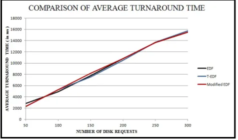
Figure 9 shows the average turnaround time for 50-300 requests. Here again, Modified EDF results in shorter turnaround time when the load on the system is light as well as during high load condition.
Figure 9. Comparison of average turnaround time of EDF, T-EDF and Modified EDF
Table II. Summary of the results of EDF, T-EDF and Modified EDF
Seek Time
Algorithm
Type of Load
Light (50-100)
Medium (100-200)
Heavy (200-300) EDF Same as T-EDF Moderate Lowest
T-EDF
Slightly higher than Modified EDF
Lowest Highest
Modified
EDF Lowest Highest Same as EDF Average Waiting Time
EDF Same as T-EDF Moderate Lower than T-EDF
T-EDF
Slightly higher than Modified EDF
Lowest
Slightly higher than Modified EDF Modified
EDF Lowest Highest Lower than EDF Average Turnaround Time
EDF Same as T-EDF Moderate Lower than T-EDF
T-EDF
Slightly more than Modified EDF
Lowest
Slightly higher than Modified EDF Modified
EDF Lowest Highest Lower than EDF
b) SCAN-EDF, TSCAN-EDF and Modified SCAN-EDF
Figure 10. Comparison of seek time of SCAN-EDF, TSCAN-EDF and Modified SCAN-EDF
Figure 11 shows the average waiting time for 50-300 requests. Here, Modified SCAN-EDF results in shorter waiting time when the load on the system is light as well as during high load condition.
Figure 11. Comparison of average waiting time of SCAN-EDF, TSCAN-EDF and Modified SCAN-TSCAN-EDF
Figure 12 shows the average turnaround time for 50-300 requests. Modified SCAN-EDF results in shorter turnaround time when the load on the system is light as well as during high load condition but turnaround time increases when the system is medium loaded.
Figure 12. Comparison of average turnaround time of SCAN-EDF, TSCAN-EDF and Modified SCAN-EDF
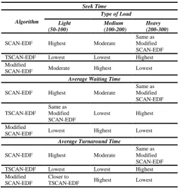
Table III. Summary of the results of SCAN-EDF, TSCAN-EDF and MODIFIED SCAN-EDF
Seek Time
Algorithm
Type of Load
Light (50-100)
Medium (100-200)
Heavy (200-300)
SCAN-EDF Highest Moderate
Same as Modified SCAN-EDF TSCAN-EDF Lowest Lowest Highest Modified
SCAN-EDF Moderate Highest Lowest Average Waiting Time
SCAN-EDF Highest Moderate
Same as Modified SCAN-EDF
TSCAN-EDF
Same as Modified SCAN-EDF
Lowest Highest
Modified
SCAN-EDF Lowest Highest Lowest Average Turnaround Time
SCAN-EDF Highest Moderate
Same as Modified SCAN-EDF TSCAN-EDF Lowest Lowest Highest Modified
SCAN-EDF
Closer to
TSCAN-EDF Highest Lowest
c) SSEDO, T-SSEDO and Modified SSEDO
Figure 13 shows the seek time graph of SSEDO, T-SSEDO and Modified SSEDO. As depicted in the graph, during light loads all the three algorithms initially perform at the same level with Modified SSEDO slightly improving the seek time. As the system load increases, it is observed that the original SSEDO algorithm performs better than our modified versions.
Figure 13. Comparison of seek time of SSEDO, T-SSEDO and Modified SSEDO
Figure 14. Comparison of average waiting time of SSEDO, T- SSEDO and Modified SSEDO
Figure 15 shows the average turnaround time of SSEDO, T-SSEDO and Modified SSEDO over 50-300 requests. Modified SSEDO results in shorter turnaround time when the load on the system is light. However the performance of SSEDO algorithm is better than the modified ones when the load on the system is increased.
Figure 15. Comparison of average turnaround time of SSEDO, T-SSEDO and Modified SSEDO
Table IV. Summary of the results of SSEDO, T-SSEDO and MODIFIED
SSEDO
Seek Time
Algorithm
Type of Load
Light (50-100)
Medium (100-200)
Heavy (200-300)
SSEDO Highest Lowest Lowest
T-SSEDO Lowest High Highest
Modified SSEDO
Same as T-SSEDO
Slightly higher
than T-SSEDO Moderate Average Waiting Time
SSEDO Highest Lowest Lowest
T-SSEDO Lowest High Highest
Modified SSEDO
Same as T-SSEDO
Slightly higher
than T-SSEDO Moderate Average Turnaround Time
SSEDO Highest Lowest Lowest
T-SSEDO Lowest High Highest
Modified SSEDO
Same as T-SSEDO
Slightly higher
than T-SSEDO Moderate
d) SSEDV, T-SSEDV and Modified SSEDV
Figure 16 shows the seek time graph of SSEDV, T-SSEDV and Modified SSEDV. As depicted in the graph, it can be observed that the original SSEDV algorithm performs better than our proposed algorithms.
Figure 16. Comparison of seek time of SSEDV, T-SSEDV and Modified SSEDV
Figure 17 shows the average waiting time of SSEDV, T-SSEDV and Modified T-SSEDV over 50-300 requests. Here, Modified SSEDV results in shorter waiting time when the load on the system is light. Both the SSEDV and Modified SSEDV algorithms perform at nearly the same level as the number of incoming requests increases.
Figure 17. Comparison of average waiting time of SSEDV, T-SSEDV and Modified SSEDV
Figure 18 shows the average turnaround time of SSEDV, T-SSEDV and Modified SSEDV over 50-300 requests. Modified SSEDV results in shorter turnaround time when the load on the system is light. However the SSEDV algorithm performs better than the proposed algorithms as the number of incoming requests increases.
Table V. Summary of the results of SSEDV, T-SSEDV and MODIFIED
T-SSEDV Highest Highest Highest Modified Average Waiting Time
SSEDV Highest Lowest Lowest
T-SSEDV
Same as Modified SSEDV
Highest Highest
Modified
SSEDV Lowest Moderate
Slightly higher than SSEDV Average Turnaround Time
SSEDV Highest Lowest Lowest
T-SSEDV
Same as Modified SSEDV
Highest Highest
Modified
SSEDV Lowest Moderate
Slightly higher than SSEDV
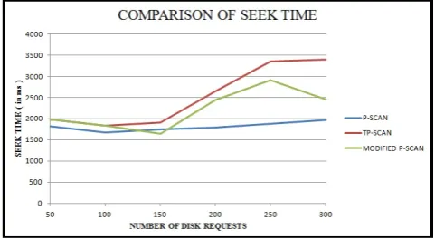
e) P-SCAN, TP-SCAN and Modified P-SCAN
From the graph in Figure 19, it is clear that the original P-SCAN algorithm outperforms our proposed algorithms as far as seek time is concerned. Both the TP-SCAN and Modified P-SCAN algorithms result in high seek times.
Figure 19. Comparison of seek time of P-SCAN, TP-SCAN and Modified P-SCAN
Figure 20 shows the average waiting time of P-SCAN, TP-SCAN and Modified P-TP-SCAN over 50-300 requests. P-TP-SCAN results in higher average waiting time. TP-SCAN and Modified P-SCAN perform moderately well during light loads, the latter being slightly better during heavy loads.
Figure 20. Comparison of average waiting time of P-SCAN, TP-SCAN and Modified P-SCAN
Figure 21 shows the average turnaround time of P-SCAN, TSCAN and Modified SCAN over 50-300 requests. P-SCAN results in higher average turnaround time. TP-P-SCAN and Modified P-SCAN perform moderately well during light loads, the latter being slightly better during heavy loads.
Figure 21. Comparison of average turnaround time of P-SCAN, TP-SCAN and Modified P-TP-SCAN
Table VI. Summary of the results of P-SCAN, TP-SCAN and MODIFIED P-SCAN TP-SCAN Highest Highest Highest Modified
P-SCAN
Same as
TP-SCAN Moderate Moderate Average Waiting Time
P-SCAN Highest Highest Highest
TP-SCAN Lowest
Same as
Average Turnaround Time
P-SCAN Highest Highest Highest
TP-SCAN Lowest
V. CONCLUSION
Tardiness is an important yardstick to measure the performance of a soft real time system. Keeping this in mind, modifications to existing algorithms have been proposed. Based on our simulation study, we observe that our proposed algorithms perform better compared to most of the existing algorithms even when we take tardiness into account. Compared to P-SCAN, which gives the best result with respect to existing algorithms, our algorithm outperforms it with respect to service time since average waiting time as well as average turnaround time are lower.
VI. FUTURE WORK
We plan to model the disk behaviour more in tune with an actual working environment- for example, taking device queuing time and channel wait time into account in our simulation.
VII. REFERENCES
[1] Celis, J.R., Gonzales, D., Lagda, E., and Rutaquio Jr., L.,“A Comprehensive Review for Disk Scheduling
Algorithms”, International Journal of Computer Science Issues, Vol. 11, No. 1, 74-79, January 2014.
[2] Stallings, W., Computer Organization and Architecture- Designing For Performance, Seventh Edition, Pearson, 2007.
[3] Liu, C. L., and Layland, J. W., “Scheduling Algorithms for Multiprogramming in a Hard-Real-Time Environment,” Journal of the Association for Computing Machinery, Vol. 20, No.1, 44-61, January 1973.
[4] Reddy, A. L. N., and Wyllie, J.C., “Disk Scheduling in a Multimedia I/O System”, Proceedings of the ACM Multimedia Conference, 225-233, August 1993.
[5] Carey, M.J., Jauhari, R., and Livny, M., “Priority in DBMS Resource Scheduling”, Proceedings of the 15th VLDB Conference, 397-410, August 1989.
[6] Chen, S., Stankovic, J.A., Kurose, J.F., and Towsley, D.F,”Performance Evaluation of Two New Disk Scheduling algorithms for Time Systems”, Real-Time Systems, Vol. 3, No. 3, 307-336, 1991.
![Figure 1. Disk Structure[1]](https://thumb-us.123doks.com/thumbv2/123dok_us/693011.1076866/1.595.346.536.384.555/figure-disk-structure.webp)