Affinity Measures Based on the Graph Laplacian

Coling 2008: Proceedings of 3rd Textgraphs workshop on Graph-Based Algorithms in Natural Language Processing,pages 41–48

Affinity Measures based on the Graph Laplacian

Delip Rao

Dept. of Computer Science Johns Hopkins University

[email protected]

David Yarowsky Dept. of Computer Science

Johns Hopkins University [email protected]

Chris Callison-Burch Dept. of Computer Science

Johns Hopkins University [email protected]

Abstract

Several language processing tasks can be inherently represented by a weighted graph where the weights are interpreted as a measure of relatedness between two ver-tices. Measuring similarity between ar-bitary pairs of vertices is essential in solv-ing several language processsolv-ing problems on these datasets. Random walk based measures perform better than other path based measures like shortest-path. We evaluate several random walk measures and propose a new measure based on com-mute time. We use the psuedo inverse of the Laplacian to derive estimates for commute times in graphs. Further, we show that this pseudo inverse based mea-sure could be improved by discarding the least significant eigenvectors, correspond-ing to the noise in the graph construction process, using singular value decomposi-tion.

1 Introduction

Natural language data lend themselves to a graph based representation. Words could be linked by explicit relations as in WordNet (Fellbaum, 1989) or documents could be linked to one another via hyperlinks. Even in the absence of such a straight-forward representation it is possible to derive meaningful graphs such as the nearest neighbor graphs as done in certain manifold learning meth-ods (Roweis and Saul, 2000; Belkin and Niyogi,

c

°2008. Licensed under the Creative Commons Attribution-Noncommercial-Share Alike 3.0 Unported li-cense (http://creativecommons.org/licenses/by-nc-sa/3.0/). Some rights reserved.

2001). All of these graphs share the following properties:

• They are edge-weighted.

• The edge weight encodes some notion of re-latedness between the vertices.

• The relation represented by edges is at least weakly transitive. Examples of such rela-tions include, “is similar to”, “is more general than”, and so on. It is important that the re-lations selected are transitive for the random walk to make sense.

Such graphs present several possibilities in solv-ing language problems on the data. One such task is, given two vertices in the graph we would like to know how related the two vertices are. There is an abundance of literature on this topic, some of which will be reviewed here. Finding similarity between vertices in a graph could be an end in it-self, as in the lexical similarity task, or could be a stage before solving other problems like clustering and classification.

2 Contributions of this paper The major contributions of this paper are

• A comprehensive evaluation of various ran-dom walk based measures

• Propose a new similarity measure based on commute time.

• An improvement to the above measure by eliminating noisy features via singular value decomposition.

3 Problem setting

Consider an undirected graph G(V, E,W) with verticesV, edgesE, andW = [wij]be the sym-metric adjacency weight matrix with wij as the weight of the edge connecting verticesiandj. The weight, wij = 0 for verticesi andj that are not neighbors and whenwij >0it is interpreted as an indication of relatedness betweeniandj. In our case, we consider uniformly weighted graphs, i.e, wij = 1for neighbors but this need not be the case. Letn= |V|be the order of the graph. We define a relationsim :V ×V → R+ _{such thatsim(i, j)}

is the relatedness between verticesiandj. There are several ways to definesim; the ones explored in this paper are:

• sim_G(i, j) is the reciprocal of the shortest path length between vertices i and j. Note that this is not a random walk based mea-sure but a useful baseline for comparison pur-poses.

• simB(i, j)is the probability of a random walk from vertex i to vertex j using all paths of length less thanm.

• sim_P(i, j)is the probability of a random walk from vertexito vertexjdefined via a pager-ank model.

• sim_C(i, j)is a function of the commute time between vertexiand vertexj.

4 Data and Evaluation

We evaluate each of the similarity measure we consider by using a linguistically motivated task of finding lexical similarity. Deriving lexical relatedness between terms has been a topic of interest with applications in word sense disam-biguation (Patwardhan et al., 2005), paraphras-ing (Kauchak and Barzilay, 2006), question an-swering (Prager et al., 2001), and machine trans-lation (Blatz et al., 2004) to name a few. Lex-ical relatedness between terms could be derived either from a thesaurus like WordNet or from raw monolingual corpora via distributional simi-larity (Pereira et al., 1993). WordNet is an inter-esting graph-structured thesaurus where the ver-tices are the words and the edges represent rela-tions between the words. For the purpose of this work, we only consider relations like hypernymy, hyponymy, and synonymy. The importance of this

problem has generated copious literature in the past – see (Pedersen et al., 2004) or (Budanitsky and Hirst, 2006) for a detailed review of various lexical relatedness measures on WordNet. Our fo-cus in this paper is not to derive the best similar-ity measure for WordNet but to use WordNet and the lexical relatedness task as a method to evalu-ate the various random walk based similarity mea-sures. Following the tradition in previous litera-ture we evaluate on the Miller and Charles (1991) dataset. This data consists of 30 word-pairs along with human judgements which is a real value be-tween 1 and 4. For every measure we consider, we derive similarity scores and compare with the human judgements using the Spearman rank cor-relation coefficient.

5 Graph construction

For the purpose of evaluation of the random walk measures, we construct a graph for every pair of words for which similarity has to be computed. This graph is derived from WordNet as follows:

• For each wordwin the pair(w1, w2):

– Add an edge between w and all of its parts of speech. For example, if the word is coast, add edges betweencoastand

coast#nounandcoast#verb.

– For each word#pos combination, add edges to all of its senses (For example, coast#noun#1 through

coast#noun#4.

– For each word sense, add edges to all of its hyponyms

– For each word sense, add edges to all of its hypernyms recursively.

In this paper we consider uniform weights on all edges as our main aim is to illustrate the differ-ent random walk measures rather than fine tune the graph construction process.

6 Shortest path based measure

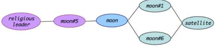
Figure 1: Shortest path distances on graphs

measure but will serve as an important baseline for our work. As can be observed from Table 1, the

Method Spearman correlation

Geodesic 0.275

Table 1: Similarity using shortest-path measure.

correlation is rather poor for the shortest path mea-sure.

7 Why are shortest path distances bad? While shortest-path distances are useful in many applications, it fails to capture the following obser-vation. Consider the subgraph of WordNet shown in Figure 1. The term moon is connected to the terms religious leader and satellite1_.

Observe that both religious leader and

satellite are at the same shortest path dis-tance from moon. However, the connectivity structure of the graph would suggestsatellite

to be “more” similar than religious leader

as there are multiple senses, and hence multiple paths, connectingsatelliteandmoon.

Thus it is desirable to have a measure that cap-tures not only path lengths but also the connectiv-ity structure of the graph. This notion is elegantly captured using random walks on graphs.

7.1 Similarity via Random walks

A random walk is a stochastic process that consists of a sequence of discrete steps taken at random de-fined by a distribution. Random walks have inter-esting connections to Brownian motion, heat diffu-sion and have been used in semi-supervised learn-ing – for example, see (Zhu et al., 2003). Certain properties of random walks are defined for ergodic processes only2_{. In our work, we assume these} 1_{Thereligious leadersense ofmoonis due to Sun} Myung Moon, a US religious leader.

2_{A stochastic process is ergodic if the underlying Markov} chain is irreducible and aperiodic. A Markov chain is

irre-hold true as the graphs we deal with are connected, undirected, and non-bipartite.

7.1.1 Bounded length walks

As our first random walk measure, we consider the bounded length walk – i.e., all random walks of length less than or equal to a boundm. We derive a probability transition matrixP from the weight matrixWas follows:

P=D−1W

where, D is a diagonal matrix with dii = P_n

j= 1wij. Observe that:

• pij =P[i, j]≥0, and

• Pn_{j= 1}pij = 1

Hence pij can be interpreted as the probability of transition from vertexito vertexjin one step. It is easy to observe thatPk_{gives the transition} prob-ability from vertexi to vertexj in k steps. This leads to the following similarity measure:

S=P+P2+P3+...+Pm

Observe thatS[i, j]derives the total probability of transition from vertex ito vertex j in at most m steps3_{. GivenS, we can derive several measures of}

similarity:

1. Bounded Walk:S[i, j]

2. Bounded Walk Cosine: dot product of rowvectorsSiandSj.

When we evaluate these measures on the Miller-Charles data the results shown in Table 2. are ob-served. For this experiment, we consider all walks that are at most 20 steps long, i.e., m = 20. Ob-serve that these results are significantly better than the Geodesic similarity based on shortest-paths. ducible if there exists a path between any two states and it is aperiodic if the GCD of all cycle lengths is one.

Method Spearman correlation

Bounded Walk 0.346

Bounded Walk Cosine 0.365

Table 2: Similarity using bounded random walks (m= 20).

7.1.2 How many paths are sufficient?

In the previous experiment, we arbitrarily fixed m = 20. However, as observed in Figure 2. , be-yond a certain value the choice ofmdoes not affect the result as the random walk converges to its sta-tionary distribution. The choice ofm depends on

Figure 2: Effect ofmin Bounded walk

the amount of computation available. A reason-ably large value ofm (m > 10) should be suffi-cient for most purposes and one could use lower values of m to derive an approximation for this measure. One could derive an upper bound on the value ofmusing the mixing time of the underlying Markov chain (Aldous and Fill, 2001).

7.1.3 Similarity via pagerank

Pagerank (Page et al., 1998) is the celebrated ci-tation ranking algorithm that has been applied to several natural language problems from summa-rization (Erkan and Radev, 2004) to opinion min-ing (Esuli and Sebastiani, 2007) to our task of lexical relatedness (Hughes and Ramage, 2007). Pagerank is yet another random walk model with a difference that it allows the random walk to “jump” to its initial state with a nonzero probability (α). Given the probability transition matrixPas defined above, a stationary distribution vector for any ver-tex (sayi) could be derived as follows:

1. Leteibe a vector of all zeros withei(i) = 1

2. Letv0=ei

3. Repeat untilkvt−vt−1kF < ²

• vt+1=αvtP+ (1−α)v0

• t=t+ 1

4. Assignvt+1 as the stationary distribution for

vertexi.

Armed with the stationary distribution vectors for verticesiandj, we define pagerank similarity ei-ther as the cosine of the stationary distribution vec-tors or the reciprocal Jensen-Shannon (JS) diver-gence4 _{between them. Table 3. shows results on}

the Miller-Charles data. We useα = 0.1, the best value on this data. Observe that these results are Method Spearman correlation

Pagerank JS-Divergence 0.379

Pagerank Cosine 0.393

Table 3: Similarity via pagerank (α= 0.1).

better than the best bounded walk result. We fur-ther note that our results are different from that of (Hughes and Ramage, 2007) as they use exten-sive feature engineering and weight tuning during the graph generation process that we have not been able to reproduce. Hence for simplicity we stuck to a simpler graph generation process. Nevertheless, the result in Table 3. is still useful as we are in-terested in the performance of the various spectral similarity measures rather than achieving the best performance on the lexical relatedness task. The graphs we use in all methods are identical making comparisons across methods possible.

7.2 Similarity via Hitting Time

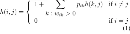
Given a graph with the transition probability ma-trixP as defined above, the hitting time between verticesi andj, denoted ash(i, j), is defined as the expected number of steps taken by a random walker to first encounter vertexjstarting from ver-texi. This can be recursively defined as follows:

h(i, j) =   

1 + X

k:wik >0

pikh(k, j) ifi6=j

0 ifi=j

(1)

4_{The Jensen-Shannon divergence between two} distribu-tionspandqis defined asD(pka)+D(qka), whereD(.k

The lower the hitting times of two vertices, the more similar they are. It can be easily verified that hitting time is not a symmetric relation hence graph theory literature suggests another symmet-ric measure – the commute time.5 _{The commute}

time,c(i, j), is the expected number of steps taken to leave vertexi, reach vertexj, and return back to i. Thus,

c(i, j) =h(i, j) +h(j, i) (2)

Observe that, the commute time is a metric in that it is positive definite, symmetric, and satisifies tri-angle inequality. Hence, commute time could be used as a distance measure as well. We derive a similarity measure from this distance measure us-ing the followus-ing lemma.

Lemma 1. For every edge (i, j), c(i, j) ≤ 2l

wherel=|E|, the number of edges.

Proof. This can be easily observed by defining a Markov chain on the edges with probability tran-sition matrix Qwith2lstates, such thatQe1e2 =

1/degree(e1 ∩e2). Since this matrix is doubly

stochastic, the stationary distribution on this chain will be uniform with a probability 1/2l. Now c(i, j) =h(i, j)+h(j, i), is the expected time for a walk to start ati, visitj, and return back toi. When the stationary probability at each edge is1/2l, this expected time evaluates to2l. Hence the commute time can be at most2l.

This lemma allows us to define a similarity mea-sure as follows:

simC(i, j) = 1− c(i, j_2l ) (3)

Observe that the measure defined in Equation 3 is a metric and further its range is defined in [0,1]. We now only need a way to compute the commute times to use Equation 3. One could compute the hitting times and hence the commute times from the Equations 1 and 2 using dynamic program-ming, akin to shortest paths in graphs. In this pa-per, we instead choose to derive commute times via the graph Laplacian. This also allows us to handle “noise” in the graph construction process which cannot be taken care by naive dynamic pro-gramming.

5_{Note that distance measures, in general, need not be} sym-metric but we interpret distance as proximity which mandates symmetry.

Chandra et. al. (1989) show that the commute time between two vertices is equal to the resis-tance disresis-tance between them. Resisresis-tance disresis-tance, as proposed by Klein and Randic (1993), is the effective resistance between two vertices in the electrical network represented by the graph, where the edges have resistance 1/wij. Xiao and Gut-man (2003), show the relation between resistance distances in graphs to the Laplacian spectrum, thus enabling a way to derive commute times from the graph Laplacian in closed form.

We now introduce graph Laplacians, which are interesting in their own right besides being related to commute time. The Laplacian of a graph could be viewed as a discrete version of the Laplace-Beltrami operator on Riemannian manifolds. It is defined as

L=D−W

The graph Laplacian has interesting properties and a wide range of applications, in semi-supervised learning (Zhu et al., 2003), non-linear dimension-ality reduction (Roweis and Saul, 2000; Belkin and Niyogi, 2001), and so on. See (Chung, 1997) for a thorough introduction on Laplacians and their properties. We depend on the fact thatLis:

1. symmetric (sinceDandW are for undirected graphs)

2. positive-semidefinite : since it is symmet-ric, all of the eigenvalues are real and by the Greshgorin circle theorem, the eigenval-ues must also be non-negative and henceLis positive-semidefinite.

Throughout this paper we use normalized Lapla-cians as defined below:

L=D−1/2_LD−1/2 _=I−D−1/2_WD−1/2

The normalized Laplacians preserve all properties of the Laplacian by construction.

As noted in Xiao and Gutman (2003), the re-sistance distances can be derived from the gener-alized Moore-Penrose pseudo-inverse of the graph Laplacian(L†_{) – also called the inverse Laplacian.}

Like Laplacians, their pseudo inverse counterparts are also symmetric, and positive semi-definite. Lemma 2. L†_{is symmetric}

property of graph Laplacians, LT _{= L. Hence,} (L†₎T _=L†_.

Lemma 3. L†_{is positive semi-definite}

Proof. We make use of the following properties from (Chung, 1997):

• The Laplacian, L, is positive semi-definite (also shown above).

• If the Eigen-decomposition of L is QΛQT_, then the Eigen-decomposition of the pseudo-inverseL†_isQΛ−1_QT_{. If any of the} eigenval-ues ofLis zero then the corresponding eigen-value forL†_{is also zero.}

Since L is positive semi-definite, and the eigen-values ofL† _{have the same sign asL, the pseudo}

inverseL†_{has to be positive semi-definite.}

Lemma 4. The inverse Laplacian is a gram matrix Proof. To prove this, we use the fact that the Laplacian Matrix is symmetric and positive semi-definite. Hence by Cholesky decomposition we can writeL=UUT_.

ThereforeL†_{= (U}T₎†_U†_{= (U}†₎T_(U†_).

HenceL†_{is a matrix of dot-products or a}

gram-matrix.

Thus, from Lemmas 2, 3 and 4, the inverse LaplacianL†_{is a valid Kernel.}

7.2.1 Similarity measures from the Laplacian The pseudo inverse of the Laplacian allows us to compute the following similarity measures.

1. SinceL†_{is a kernel,L}†

ij can be interpreted a similarity value of verticesiandj.

2. Commute time: This is due to (Aldous and Fill, 2001). The commute time, c(i, j) ∝

(L†_ii+L†_jj −2L†_ij). This allows us to derive similarities using Equation 3.

Evaluating the above measures with the Miller-Charles data yields results shown in Table 4. Again, these results are better than the other ran-dom walk methods compared in the paper.

Method Spearman correlation

L†_ij 0.469

Commute Time (simC) 0.520

Table 4: Similarity via inverse Laplacian.

7.2.2 Noise in the graph construction process The graph construction process outlined in Sec-tion 5 is not necessarily the best one. In fact, any method that constructs graphs from existing data incorporates “noise” or extraneous features. These could be spurious edges between vertices, miss-ing edges, or even improper edge weights. It is however impossible to know any of this a priori and some noise is inevitable. The derivation of commute times via the pseudo inverse of a noisy Laplacian matrix makes it even worse because the pseudo inverse amplifies the noise in the original matrix. This is because the largest singular value of the pseudo inverse of a matrix is equal to the in-verse of thesmallestsingular value of the original matrix. A standard technique in signal processing and information retrieval to eliminate noise or han-dle missing values is to use singular value decom-position (Deerwester et al., 1990). We apply SVD to handle noise in the graph construction process.

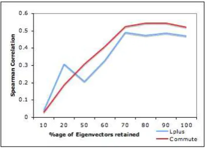
For a given matrix A, SVD decomposesAinto three matricesU, S, andV such thatA =USVT_, whereSis a diagonal matrix of eigenvalues ofA, andU andV are orthonormal matrices containing the left and the right eigenvectors respectively. The top-k eigenvectors and eigenvalues are computed using the iterative method by Lanczos-Arnoldi (us-ing LAPACK) and the product of these matrices represents a “smoothed” version of the original Laplacian. The pseudo inverse is then computed on this smooth Laplacian. Table 5., shows the im-provements obtained by discarding bottom 20% of the eigenvalues.

Method Original After SVD

L†_ij 0.469 0.472

Commute Time (simC) 0.520 0.542

Table 5: Denoising graph Laplacian via SVD

Figure 3. shows the dependence on the num-ber of eigenvalues selected. As can be observed in both curves there is a reduction in performance by adding the last few eigenvectors and hence may be safely discarded. This observation is true in other text processing tasks like document clustering or classification using Latent Semantic Indexing.

8 Related Work

Figure 3: Noise reduction via SVD.

et al (2007) on using sigmoid commute time kernel on a graph for document clustering but our work differs in that our goal was to study various ran-dom walk measures rather than a specific task and we provide a new similarity measure (ref. Eqn 3) based on an upper bound on the commute time (Lemma 1). Our work also suggests a way to han-dle noise in the graph construction process. 9 Conclusions and Future Work

This paper presented an evaluation of random walk based similarity measures on weighted undi-rected graphs. We provided an intuitive explana-tion of why random walk based measures perform better than shortest-path or geodesic measures, and backed it with empirical evidence. The ran-dom walk measures we consider include bounded length walks, pagerank based measures, and a new measure based on the commute times in graphs. We derived the commute times via pseudo inverse of the graph Laplacian. This enables a new method of graph similarity using SVD that is robust to the noise in the graph construction process. Further, the inverse Laplacian is also interesting in that it is a kernel by itself and could be used for other tasks like word clustering, for example.

Acknowledgements

The authors would like to thank David Smith and Petros Drineas for useful discussions and to Fan Chung for the wonderful book on Spectral Graph theory.

References

Aldous and Fill. 2001. Reversible Markov Chains and Random Walks on Graphs. In preparation.

Belkin, Mikhail and Partha Niyogi. 2001. Laplacian eigenmaps and spectral techniques for embedding and clustering. InProceedings of the NIPS.

Blatz, John, Erin Fitzgerald, George Foster, Simona Gandrabur, Cyril Goutte, Alex Kulesza, Alberto San-chis, and Nicola Ueffing. 2004. Confidence estima-tion for machine translaestima-tion. In Proceeding of the COLING.

Budanitsky, Alexander and Graeme Hirst. 2006. Eval-uating wordnet-based measures of lexical semantic relatedness. Computational Linguistics, 32(1):13– 47.

Chandra, Ashok, Prabhakar Raghavan, Walter Ruzzo, Roman Smolensky, and Prasoon Tiwari. 1989. The electrical resistance of a graph captures its commute and cover times. InProceedings of the STOC.

Chung, Fan. 1997. Spectral graph theory. InCBMS: Conference Board of the Mathematical Sciences, Re-gional Conference Series.

Deerwester, Scott, Susan Dumais, George Furnas, Thomas Landauer, and Richard Harshman. 1990. Indexing by latent semantic analysis. Journal of the American Society for Information Science, 41.

Erkan, G¨unes and Dragomir Radev. 2004. Lexrank: Graph-based lexical centrality as salience in text summarization.Journal of Artificial Intelligence Re-search (JAIR), 22:457–479.

Esuli, Andrea and Fabrizio Sebastiani. 2007. Pager-anking wordnet synsets: An application to opinion mining. InProceedings of the ACL, pages 424–431.

Fellbaum, Christaine, editor. 1989. WordNet: An Elec-tronic Lexical Database. The MIT Press.

Hughes, Thad and Daniel Ramage. 2007. Lexical semantic relatedness with random graph walks. In

Proceedings of the EMNLP.

Kauchak, David and Regina Barzilay. 2006. Para-phrasing for automatic evaluation. InProceedings HLT-NAACL.

Klein, D. and M. Randic. 1993. Resistance distance.

Journal of Mathematical Chemistry, 12:81–95.

Lin, Jianhua. 1991. Divergence measures based on the shannon entropy.IEEE Transactions on Information Theory, 37(1).

Miller, G. and W. Charles. 1991. Contextual correlates of semantic similarity. InLanguage and Cognitive Process.

Patwardhan, Siddharth, Satanjeev Banerjee, and Ted Pedersen. 2005. Senserelate:: Targetword-A gen-eralized framework for word sense disambiguation. InProceedings of the ACL.

Pedersen, Ted, Siddharth Patwardhan, and Jason Michelizzi. 2004. Wordnet::similarity - measuring the relatedness of concepts. InProceedings of the AAAI.

Pereira, Fernando, Naftali Tishby, and Lillian Lee. 1993. Distributional clustering of english words. In

Proceedings of the ACL.

Prager, John M., Jennifer Chu-Carroll, and Krzysztof Czuba. 2001. Use of wordnet hypernyms for an-swering what-is questions. In Proceedings of the Text REtrieval Conference.

Roweis, Sam and Lawrence Saul. 2000. Nonlinear di-mensionality reduction by locally linear embedding.

Science, 290:2323–2326.

Xiao, W. and I. Gutman. 2003. Resistance distance and laplacian spectrum. Theoretical Chemistry Associa-tion, 110:284–289.

Yen, Luh, Francois Fouss, Christine Decaestecker, Pas-cal Francq, and Marco Saerens. 2007. Graph nodes clustering based on the commute-time kernel. In

Proceedings of the PAKDD.