Optimization of Wastewater Treatment Design under Uncertainty and Variability

ABSTRACT

DOBY, JR., TROY ALVIN. Optimization of Wastewater Treatment Design

under Uncertainty and Variability. (Under the direction of John W. Baugh, Jr.)

The objective in domestic wastewater treatment is to provide a low cost process

that is reliable meeting effluent quality standards. Designers using traditional

steady-state design and modeling of domestic wastewater treatment plants use scalar values as

inputs. The inputs are typically of two types – (1) design loadings based on historical

data and (2) stoichiometric and kinetic parameters based on literature values. Using the

traditional design approach, there is no way of knowing

a priori

the reliability of the

design or whether the design is least cost.

Designers using deterministic optimization and modeling of domestic wastewater

treatment plants also use the two types of scalar inputs as with traditional design. While

the designer may now know that the design is least cost given the inputs, there is no way

of knowing

a priori

whether the design is the most reliable for the cost.

It is possible to take an existing design – whether obtained by traditional design

methods, deterministic optimization, or by any other design method – and determine the

reliability of the design. To do so, however, requires characterization of both uncertainty

and variability of the data. Uncertainty arises because of a lack of knowledge about an

input value and its statistical distribution. Variability arises because of the heterogeneity

of the processes determining the input value and its statistical distribution. In a case

study developed herein, the historical input loadings are presented and the variability is

characterized. The characterization of the load variability is then used for future

particular case are not typically known and thus are uncertain. An approach to

quantifying the uncertainty of these values is proposed.

Different loading criteria (based on percentiles of historical flow and waste

concentration data) are used in deterministic optimization. It is determined that the

higher the flow percentile, the more expensive the design. However, a more reliable

design could be found at a lower cost and at a lower flow percentile.

A different design procedure using stochastic programming is illustrated taking

both cost and reliability into account during the design procedure. As a result, a

reliability-cost tradeoff curve is generated. This curve is characterized by (1) a steep

portion where slight increases in cost lead to large improvements in reliability; and (2) a

flat portion where large increases in cost lead to small improvements in reliability. This

design procedure also allows determination of the value of an experimental program

characterizing the uncertainty and variability of the stoichiometric and kinetic parameters

and their statistical distribution. This proposed methodology allows the designer to

choose for a level of uncertainty in stoichiometric and kinetic parameter the design values

with an optimum cost-reliability tradeoff. This proposed methodology also shows the

value to the owner of reducing the uncertainty level by experimentally determining the

Optimization of Wastewater Treatment Design

under Uncertainty and Variability

by

Troy Alvin Doby, Jr.

A dissertation submitted to the Graduate Faculty of

North Carolina State University

in partial fulfillment of the

requirements for the Degree of

Doctor of Philosophy

Department of Civil Engineering

Raleigh

2004

Approved By:

Dr. J. W. Baugh, Jr.

Dr. F. L. de los Reyes, III

Chair of Advisory Committee

Dr. S. R. Ranjithan

Dr. E. D. Brill, Jr.

BIOGRAPHY

Table of Contents

Page

List of Tables ... vi

List of Figures ... ix

Chapter 1. Introduction ...1

Chapter 2. Literature Review...3

Uncertainty

and

Variability...3

Reliability...7

Optimization under uncertainty ...7

Stochastic

Optimization

and Stochastic Programming...11

Applications of Chance-Constrained, Stochastic Optimization, and

Stochastic Programming ...13

Final

Remarks ...17

Chapter 3. Optimization of Wastewater Treatment Design under Variable Loading

Conditions with Uncertain Parameter Values: Conceptual Model ...18

Introduction...18

Traditional

Design ...20

Deterministic Optimization Design ...24

Framework for Optimization under Variability and Uncertainty ...29

Chapter 4. Loadings and Variability...33

Introduction...33

Data and Distribution...33

Fitting the Influent Concentration Data ...37

Dilution

Effects...41

Generation of Synthetic Loads...49

Final

Remarks ...56

Chapter 5. Parameter Values and Uncertainty...58

Introduction...58

Chapter 6. Deterministic Optimization and Reliability ...63

Introduction...63

Materials and Methods...63

Computers

used...63

Biological Process Used ...63

Wastewater

treatment

model

used ...64

Effluent Limits permitted...64

Raw influent data ...64

Design loadings used ...64

Stoichiometric and Kinetic Parameters used ...66

Cost

model

used...66

Objective Functions, Constraints, and Decision Variables...77

Reliability

Determination...78

Synthetic

Loading

Data

used for Simulation and Reliability

Determination ...78

Definition

of

Reliability...80

Stoichiometric and Kinetic Parameter Uncertainty

Treatment ...80

Other

Simulation

Issues ...81

Results

and

Discussion ...83

Least Cost Solutions ...83

Reliability of Least Cost Solutions ...85

Final

Remarks ...89

Chapter 7. Optimization under Uncertainty and Variability...91

Introduction...91

Materials and Methods...92

Definition of Reliability...92

Computers

used...92

Biological Process Used ...92

Wastewater

treatment

model

used ...92

Effluent Limits permitted...92

Raw Influent Data ...92

Design loadings used ...93

Stoichiometric and Kinetic Parameters used ...93

Cost

model

used...94

Capital costs ...94

Operational

pumping

costs ...94

Operational

aeration

costs...95

Objective Functions, Constraints, and Decision Variables...95

The Genetic Algorithm (GA)...98

Reliability

Determination...100

Stoichiometric and Kinetic Parameter Uncertainty

Treatment ...101

Other

Simulation

Issues ...102

Results

and

Discussion ...104

Generation of the Reliability-Cost Tradeoff Curve for a ≤ 4.0....104

Design Characteristics of Optimum Points along Reliability-Cost

Tradeoff Curves ...107

Implications of 2.50 “a” Recycle Constraint ...108

Implications of 0.50 Unaerated Sludge Mass Fraction

Constraint...111

Reducing Parameter Uncertainty: What is it worth? ...117

Assessment of Deterministically Determined Least Cost

Designs...119

Final

Remarks

...124

Bibliography ...126

Appendices...150

Appendix 1. Tar River Regional Wastewater Treatment Plant Rocky

Mount, North Carolina. Raw Data...151

List of Tables

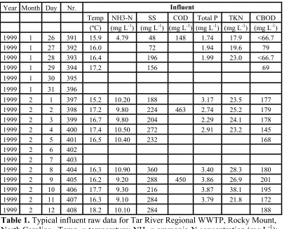
Table 1. Typical influent raw data for Tar River Regional WWTP, Rocky Mount, North

Carolina. ...34

Table 2. Raw data characterization of the Tar River Regional Wastewater Treatment

Plant (WWTP) for the 1998-2002 period ...37

Table 3. Determination of whether raw data are normally distributed ...39

Table 4. Statistical values of the mean, standard error (s. e.), the third central moment (3

c. m.), skewness, β1, fourth central moment (4

c. m.), and β2

...40

Table 5. Ammonia concentrations disaggregated by flow...44

Table 6. TKN concentrations disaggregated by flow ...44

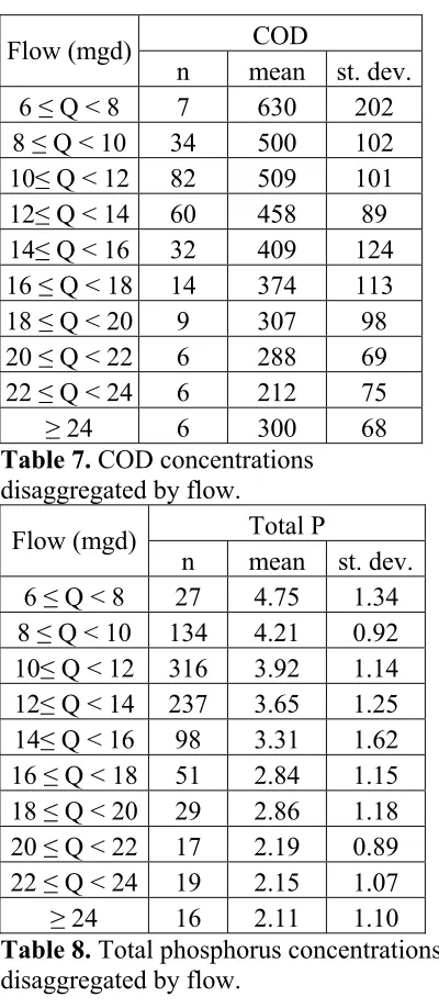
Table 7. COD concentrations disaggregated by flow. ...45

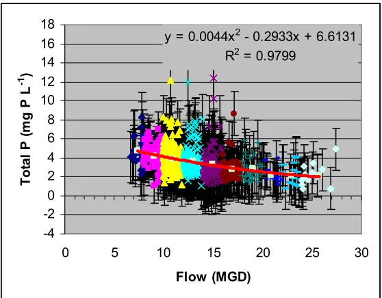
Table 8. Total phosphorus concentrations disaggregated by flow...45

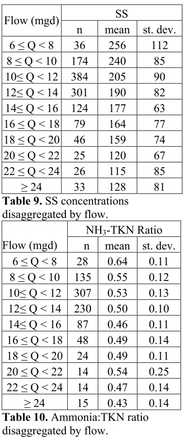
Table 9. SS concentrations disaggregated by flow ...46

Table 10. Ammonia:TKN ratio disaggregated by flow ...46

Table 11. COD:TKN ratio disaggregated by flow...50

Table 12. Total P:TKN ratio disaggregated by flow...50

Table 13. TKN standard measures (z values) assuming Pearson Type IV distributions...52

Table 14. Ammonia standard measures (z values) assuming Pearson Type IV

distributions...53

Table 15. COD standard measures (z values) assuming Pearson Type IV distributions...54

Table 16. ln(Total P) disaggregated by flow ...55

Table 17. The standard measures (z values) for normally distributed values...55

Table 18. ln(SS) disaggregated by flow...56

Table 19. Mean and standard error at different uncertainty levels of stoichiometric and

non-Arrhenius-type kinetic parameters...59

Table 21. Design loading values used in deterministic optimization based upon

percentiles of data for the Tar River Regional Wastewater Treatment Plant, Rocky

Mount, North Carolina...65

Table 22. Values of stoichiometric and kinetic parameters used in deterministic

optimization ...65

Table 23. Design flows (m3 d

_{) used in deterministic optimization...68}

Table 24. Volume (m

) reduction in biological reactors required to justify primary

clarifier...69

Table 25. Slope of head loss vs. annual cost regression lines for different diameter

pipes ...71

Table 26. Design flows (gpm) for different percentiles...71

Table 27. Cost of static head loss...72

Table 28. Friction head loss for different diameter-flow combinations ...72

Table 29. For s-recycle, cost of friction plus static head loss in different diameter pipes

for different design flow rates...74

Table 30. For a-recycle, cost of friction plus static head loss in different diameter pipes

for different design flow rates...75

Table 31. Decision variables and constraints for the least-cost optimization problem ...78

Table 32. Engineering design characteristics and annual costs of designs according to

different flow-waste characteristic percentiles ...82

Table 33. Reliability of different flow-waste concentration percentiles at 25% uncertainty

level...86

Table 34. Reliability of different designs at different uncertainty levels ...88

Table 35. Mean values of stoichiometric and kinetic parameters or functions used in their

calculation in optimization under uncertainty and variability ...93

Table 36. Decision variables and constraints for the optimization problem under

uncertainty and variability ...98

Table 38. Distribution of “a” recycle rates by percentage at different uncertainty

levels ...108

Table 39. Distribution of “s” recycle rates by percentage at different uncertainty

levels ...108

Table 40. For different uncertainty levels, percentages of “a” recycle rates falling into

different ranges ...113

Table 41. For different uncertainty levels, percentages of “s” recycle rates falling into

different ranges ...114

Table 42. For different uncertainty levels, percentages of unaerated sludge mass fraction,

smfunaerated, falling into different ranges ...115

Table 43. Approximate cost ($millions) for different reliabilities at various uncertainty

levels ...118

Table 44. Approximate reliabilities for different costs at various uncertainty levels...118

Table 45. Annual cost and engineering characteristics of least-cost deterministic

List of Figures

Figure 1. Schematic of 5-stage Bardenpho Process...2

Figure 2. Deterministic Design Procedure...22

Figure 3. Optimization of Deterministic Design Procedure ...23

Figure 4. Reliability Assessment Methodology of an Existing Design ...27

Figure 5. Optimization with Uncertainty and Variability with penalty assessment for

reliability...31

Figure 6. Optimization with Uncertainty and Variability with no penalty assessment for

reliability and constraints on decision variables that determine cost...32

Figure 7. Flow data from Tar River Regional WWTP, 1998-2002 ...35

Figure 8. Temperature of influent wastewater. Tar River Regional WWTP, Rocky Mount,

North Carolina ...35

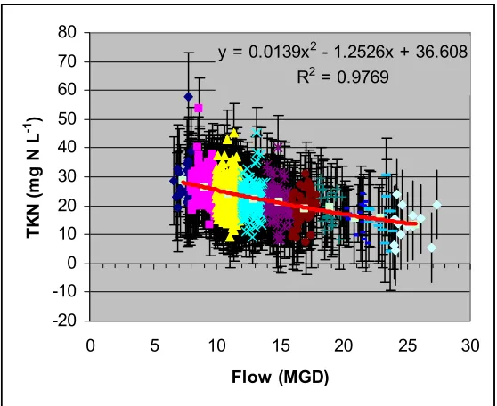
Figure 9. Normal Order Statistic Medians versus Normal Ordered Response for TKN

concentration...38

Figure 10. Dilution effect on ammonia concentration. Tar River Regional WWTP, Rocky

Mount, North Carolina...41

Figure 11. Dilution effect on TKN concentration. Tar River Regional WWTP, Rocky

Mount, North Carolina...42

Figure 12. Dilution effect on COD concentration. Tar River Regional WWTP, Rocky

Mount, North Carolina...42

Figure 13. Dilution effect on total P concentration. Tar River Regional WWTP, Rocky

Mount, North Carolina...43

Figure 14. Dilution effect on SS concentration. Tar River Regional WWTP, Rocky

Mount, North Carolina...43

Figure 15. Ammonia concentration disaggregated by flow with error bars and regression

equation...47

Figure 17. COD concentration disaggregated by flow with error bars and regression

equation...48

Figure 18. Total phosphorus concentration disaggregated by flow with error bars and

regression equation ...48

Figure 19. SS concentration disaggregated by flow with error bars and regression

equation...49

Figure 20. Schematic of 5-stage Bardenpho Process...61

Figure 21. Annual pumping costs for 1000 feet of pipe of different diameters...70

Figure 22. Annual cost for different pipe diameters per foot of head loss assuming 1,000

feet of pipe ...71

Figure 23. Partitioned GA representation with each of the decision variables as a separate

gene within the organism ...97

Figure 24. Performance of GA by generation...100

Figure 25. Reliability-Cost tradeoff curve at 0%, 5%, 10%, 20%, and 25% uncertainty

levels. Constraints: 0 ≤ smfanoxic ≤ 0.50 and 0.5 ≤ a ≤ 4.0 ...107

Figure 26. Effect of different “a” recycle constraints for 0% uncertainty level ...110

Figure 27. Effect of different “a” recycle constraints for 5% uncertainty level ...110

Figure 28. Effect of different “a” recycle constraints for 10% uncertainty level ...111

Figure 29. Effect of different “a” recycle constraints for 20% uncertainty level ...111

Figure 30. Effect of different “a” recycle constraints for 25% uncertainty level ...112

Figure 31. Reliability-Cost tradeoff curve at 0%, 5%, 10%, 20%, and 25% uncertainty

levels ...113

Figure 32. Effects of different unaerated sludge mass fraction, smfunaerated, constraints

upon annual cost and reliability at 0% uncertainty level ...116

Figure 33. Effects of different unaerated sludge mass fraction, smfunaerated, constraints

upon annual cost and reliability at 5% uncertainty level ...116

Chapter 1

Introduction

The focus of this thesis is optimization of wastewater treatment design under

uncertainty and variability. The methodology used is stochastic programming. An

example problem is developed for wastewater treatment design using data from the Tar

River Wastewater Treatment Plant in Rocky Mount, North Carolina. The process being

optimized is the 5-stage Bardenpho process, which is illustrated in Figure 1.

In Chapter 2, definitions and short literature reviews of uncertainty, variability,

reliability, and stochastic programming are provided.

In Chapter 3, the conceptual frameworks for (1) traditional wastewater treatment

design, (2) deterministic optimization of wastewater treatment design, (3) determination

wastewater treatment design reliability, and (4) optimization of wastewater treatment

design under uncertainty and variability are presented. The strengths and weaknesses of

the different frameworks are discussed.

In Chapter 4, loading values and variability are treated with presentation of the

data from the Tar River Wastewater Treatment Plant. This data shows that there are

definite dilution effects of nitrogen, COD, phosphorus, and suspended solids (SS). In

addition, the data follow an empirical distribution (Pearson Type IV). The means of

dealing with this distribution is presented.

In Chapter 5, stoichiometric and kinetic parameter values for a steady state model

are presented. Lacking any other information, the data are assumed to have a normal or

In Chapter 6, deterministic optimization of design is treated and the means of

determining the design’s reliability are presented. In this chapter it is argued that while

the reliability of a design may be determined, there is no way to assess the relative

performance of the design with regard to reliability.

In Chapter 7, design optimization under uncertainty and variability are presented

showing that with this methodology it is possible to obtain a design that is more reliable

for the same cost or less costly for the same reliability.

Figure 1. Schematic of 5-stage Bardenpho Process

Effluent

Return Activated Sludge (RAS)

“s” recycle

“a” recycle

Anoxic

Chapter 2

Literature Review

A short review of work performed in uncertainty, variability, and reliability

together with optimization under these conditions is presented. The purpose is to give

definitions of these terms and to show the methods others have used for dealing with

uncertainty, variability and reliability. Uncertainty and variability are discussed jointly

along with the techniques others have used for delineating and treating uncertainty and

variability. Optimization under uncertainty, stochastic optimization, and stochastic

programming are discussed.

Uncertainty and Variability

Three types of uncertainty are commonly designated (US EPA, 1992; Murphy,

1998):

•

Scenario uncertainty involves extending a model beyond its original bounds or

overlooking important scenarios. One example of the first type of scenario

uncertainty in wastewater treatment would be use of unmodified ASM1 for

modeling industrial wastewater treatment. An example of the second type of

scenario uncertainty would be overlooking risk of bulking/foaming when

modeling.

•

Model uncertainty involves both the structure of the model (the transport,

physical, and chemical processes involved) and not accounting for heterogeneous

conditions. Thus, in wastewater treatment modeling, the floc structure and

substrate transport would provide one level of model uncertainty while the mixing

•

Parameter uncertainty arises because of imperfect or limited knowledge.

Uncertainty may be reduced with increased knowledge. Variability, on the other

hand, arises from the heterogeneity of the data and is an inherent property of the

data. Increased knowledge does not result in decreased variability (Bennett

et al.

,

1999; Huijbregts

et al.

, 2000).

In this study, the focus will be placed on parameter uncertainty rather than model

or scenario uncertainty. Henceforth, when uncertainty is mentioned, it is implicitly

understood to mean parameter uncertainty.

Both uncertainty and variability of parameter mean values are characterized with

probability density functions (PDFs). PDFs are characterized with a distribution function

of some type, e.g., normal (or Gaussian), lognormal, gamma, chi-squared, or Weibull

distributions.

One of the most commonly used distributions is the Gaussian distribution. Its

main drawback in the context of wastewater treatment is that Gaussian distribution allows

expectations of negative values. Negative values (for concentrations, kinetics,

stoichiometries, etc.) in wastewater modeling are typically infeasible. One way around

this is use of truncated Gaussian distributions.

Lognormal distributions are also commonly used in wastewater treatment for

characterizing effluents. A justification for thinking the process gives effluent

concentrations that have lognormal distributions is that “the underlying random process is

multiplicative in nature” (Niku

et al.

, 1979). In other words, the effluent concentration

can be predicted with a nonlinear equation or set of equations. Under such

distribution of the product (effluent concentration) is lognormal (Burmaster and Hull,

1997). Furthermore, Ott (1990) demonstrated through simulation that random dilution of

an initial concentration yields a lognormally distributed final concentration.

Schmoyer

et al.

(1996), however, provide a counterargument against an

immediate assumption of lognormal distributions. Schmoyer

et al.

(1996) argue that

there is no physical reason for thinking that concentration distributions are inherently

lognormal (or any other distribution). This is because many physical processes besides

dilution shape contaminant distributions. These different physical processes are likely to

have normally-distributed measurement errors that in turn shape the concentration

distributions. Instead, Schmoyer

et al.

(1996) argue that a t-test should be used for

estimating the mean of a large series of data. Furthermore, one of the “laws” of

uncertainty analysis inveighs: “Nearly all parameter distributions of a parameter value

will look lognormal, as long as you don’t look too closely” (Hattis, 1990).

Different tools are available for assessing the distributions and the mean values of

the parameters. Efron in 1979 introduced bootstrapping for confidence interval

estimation of some known data set with n points (Efron and Tibshirani, 1993). While

there are different bootstrapping methods, the bootstrap-p method is more commonly

used for uncertainty in the mean, and is described here. A distribution function (e.g.,

Gaussian, lognormal, etc.) is assumed. A sampling technique (with replacement) is then

used to select a new set of size n drawn from the original data set. This process is then

performed r different times. The means of the r different sets are then calculated and

used for the different distribution types of the bootstrap sample imposes a distribution

and variance on the means (Cullen and Frey, 1999).

The same technique of drawing samples with replacement can be used for sample

variance. The variance values found using bootstrapping with resampling have shorter

tails than those of standard distribution functions. There is no extrapolation beyond the

boundaries of the data with variance values found with bootstrapping (Cullen and Frey,

1999).

When historical data are available, variability is probably more important than

uncertainty. The variability of the historical data can be used to generate future data. As

a result, the variability of the historical data becomes an estimate of the uncertainty of

future data (Murphy, 1998; Abdel-Aziz and Frey, 2003).

In wastewater treatment design, there usually is sufficient data to characterize the

variability of loadings that must be handled. However, there is little data available for the

characterization of the stoichiometric and kinetic parameters of a particular wastewater.

The designer is then left to use suggested values taken from the literature that may or may

not be appropriate. Knowledge of the exact stoichiometric and kinetic parameter values

that should be used requires experimental work that is not routinely performed. The

experimental methods are currently experimental, non-standardized, and expensive. As a

result, the parameter values typically used are uncertain.

Reliability

Reliability, in the current context, is the probability the proposed design will meet

historical data then is important to the extent that may provide likelihood or expectation

of future events.

Niku

et al.

(1979) used this approach to determine the reliability of meeting

effluent BOD and SS concentrations limits. BOD and SS effluent concentration data

from 37 different WWTPs were used. After raw data were collected, statistical

calculations were performed. The distributions from 25 of the 37 in both cases were

lognormal. Lognormal distribution of effluent concentrations was also in agreement with

others (Berthouex, 1974; Crain and Woods, 1995; Pöpel, 1976; Garrett, 1976).

Optimization under uncertainty

Earlier work has been performed on uncertainty in optimizing traditional

wastewater design for BOD and solids removal. However, the earlier work did not make

a distinction between uncertainty and variability. The earlier work did draw a distinction

between sensitivity analysis and uncertainty. Sensitivity analysis considers how change

in one input parameter at a time alters the expected output. Uncertainty considers how

changes in combinations of input parameter affect the output. The two different types of

techniques used in addressing parameter uncertainty can be divided into statistical and

non-statistical techniques. In the statistical approach, the mean, distribution type (normal,

uniform, triangular, etc.) and some scatter of values are provided. This is the approach

Berthouex and Polkowski (1970), Chen

et al.

(1970) and Tarrer

et al.

(1976) have used.

In the non-statistical approach, a standard for robustness is defined based on the least cost

solution and solutions that are more robust are found with an alteration of parameter

Berthouex and Polkowski (1970) optimized a wastewater treatment plant by

combining different kinetic models for different processes under conditions of model

parameter uncertainty. The decision variables were the cross-sectional areas of the

primary and secondary clarifiers, concentration of secondary clarifier underflow solids

and effluent BOD. Incorporating uncertainty (i.e., parameter standard deviations

≠

0) led

to only slight increases (3-4%) in total cost above the minimum cost without uncertainty

(i.e., parameter standard deviations = 0). The authors reported that if the BOD removal

rate was low, there was greater uncertainty in the ability to meet the effluent BOD target,

which required either increased suspended solids concentrations or increased AS basin

volume as compensation. Another finding from this study was that increasing the BOD

loading rate (kg BOD kg

VSS d

) leads to significant cost savings since the AS basin

volume can be decreased.

Chen

et al.

(1970) provided four different possible methods for incorporating

parameter sensitivity and uncertainty into the design of an optimal solution. (1)

Determining the optimal solution subject to sensitivity constraints thus ensuring that the

result would be less sensitive to parameter variations. (2) Incorporating the sensitivity

constraints into the objective function with weightings on the sensitivity functions. (3)

For parameters with fixed but uncertain values lying within certain bounds, determining

the optimum solution within the bounds of these parameters. (4) For parameters with

varying values, optimizing based on the objective function’s expected value. Chen

et al.

(1970) used the latter approach to minimize the total HRT of a two-tank-in-series CMAS

the design required larger safety factors. In almost every case, increased uncertainty led

to a reduction in the first tank’s HRT value despite an increase in total HRT.

Tarrer

et al.

(1976) optimized the design of a liquids train of a wastewater

treatment plant under parameter uncertainty. To gauge uncertainty, the authors assigned

variances to the model parameters. Monte Carlo simulation was performed with these

variances to produce expected effluent soluble BOD and SS concentrations. The

variances in the simulated results and observed values were compared. There was only a

slight difference in the variances of effluent soluble BOD concentration and no difference

in the effluent SS concentration. The cross-sectional area of the final clarifier and the

flow were set to constant values while other parameters were given stochastic values.

This study showed that both SRT and MLSS concentration values should have minimum

values placed as constraints. The authors’ most important conclusion was that when

faced with uncertainty in parameter values that would affect risk of system failure, the

best means of dealing with this was to choose extreme parameter values. This caused the

capital and operating costs to increase, but not dramatically.

Uber

et al.

(1991a) presented a “robust optimal design” framework for dealing

with parameter value uncertainty by merging optimization and sensitivity analysis. The

uncertainty considered could be from “subjective parameter estimates, measurement

errors, inadequate data, natural variability” or any combination thereof. Robustness of

the system was defined as the ability to deliver the required level of service even if the

model parameters varied from the values assumed during design. The framework was

function of changes in system performance due to parameter value changes.

Improvements in robustness resulted from decreased system sensitivity coefficient

values. A robustness function was defined as the sum of the weighted sensitivities of

each of the model parameters. Requiring the robustness function to meet a target

robustness value allowed incorporation of the robustness function into the optimization

problem as a constraint. Choice of the decision variables was important in this

framework. The decision variables should not be control variables (e.g., recycle rates)

since their inclusion would lead to a maximally conservative design. Uber

et al.

(1991b)

then used the “robust optimal design” framework for the problem and model given by

Tang

et al.

(1987a, b). There were 55 uncertain parameters in the model and robustness

was with respect to the ability to meet effluent BOD and TSS concentration values. Of

the decision variables chosen, two were control variables. As a result, the authors

asserted, the robustness measures should be “interpreted as estimates of the maximum

change in performance for a particular operating regime given by the values of the”

decision variables. Two tradeoff curves between (1) robustness of effluent BOD

concentration and cost and (2) robustness of effluent TSS concentration and cost showed

that effluent BOD was more sensitive than TSS to parameter variations. In addition,

BOD robustness could be improved greatly (~55%) with approximately a 10% cost

increase from the least cost solution. The effluent BOD concentration was most sensitive

to sludge thickening and AS kinetic parameters. The effluent TSS concentration was

most sensitive to the influent flow rate and secondary clarifier parameters. When

design. Joint robustness increases and BOD robustness increases required greater SRT

values than the least-cost SRT values. The authors concluded that not only would

increased SRT improve settleability in the secondary clarifier, as Bisogni and Lawrence

(1970) had concluded, but the increased SRT would lead to greater robustness in being

able to meet effluent BOD concentration targets.

Uncertainty analysis combined with nutrient removal remains virtually

unexplored and will be a rich field for future investigations, using both statistically-based

and non-statistically-based methods as presented above. Future questions uncertainty

analysis can address include: How often will this proposed plant meet effluent quality

standards? How do you design a plant that will meet effluent quality standards X% of the

time within a Y% confidence limit? Stochastic optimization and particularly stochastic

programming are methodologies that can be used to provide answers to such questions.

Stochastic Optimization and Stochastic Programming

Stochastic optimization and stochastic programming are two potential approaches

for addressing optimization of wastewater treatment design under uncertainty. The

stochastic optimization problem can be written as (Diwekar

et al.

, 1997):

))

,

(

(

1

z

x

u

P

Maximize

(1)

( )

(

,

)

0

2

h

x

u

=

P

to

subject

(2)

( )

(

,

)

0

3

g

x

u

≤

P

(3)

where x is a vector of decision variables, u is a vector of uncertain parameters, P1, P2,

dealing with uncertain parameters. The problem formulation using CCP is (Watanabe

and Ellis, 1994; Diwekar

et al.

, 1997):

( )

(

z

x

u

)

E

(

F

( )

u

)

P

Maximize

1

,

=

(4)

( )

(

h

x

u

≤

β

)

≥

α

P

to

subject

,

(5)

where x is the vector of decision variables, u is the decision of uncertain parameter

values, P and P1 are probabilistic functionals, z is the objective function, h is the set of

inequality constraints, and

α

and

β

are probability value vectors with 0

≤

α

≤

1 and 0

≤

β

≤

1. Thus, the probability of violating

P

(

h

( )

x

,

u

)

≤

β

for any choice of a decision

variable x must not be greater than the reliability level, 1-

α

α

typically normally distributed, random variables.

In both chance-constrained and stochastic optimization, stochastic models are

used in optimization. In stochastic programming, however, deterministic models may be

used. The stochastic programming problem may be written as (Diwekar

et al.

, 1997):

*))

,

(

(

1

z

x

u

P

Maximize

(6)

(

)

(

,

*

)

0

2

h

x

u

=

P

to

subject

(7)

(

)

(

,

*

)

0

3

g

x

u

≤

P

(8)

where x is a vector of decision variables, u* is a vector of vectors of uncertain

parameters, P1, P2, and P3 are probabilistic functionals, g is the set of inequality

constraints, and h is the set of equality constraints.

There are several features of stochastic programming that should be discussed:

multiple stages, recourse, and a horizon. For T stages, the stochastic program has

(Dupa

č

ová, 2002):

(

,..,

)

*

=

u

u

and with recourse, the decision variables change

(

x

x

)

x

*

=

,..,

(10)

The sequence of decisions with recourse is recursive and can then be written as:

(

,

)

,..,

(

,

,..,

)

,

,

1

u

x

x

u

x

x

u

u

x

(11)

The horizon is typically the number of stages in the problem.

In stochastic programming, there should be a tension between reducing the size of

x* or T, on the one hand, and finding a solution that is robust for small input value

changes. The problem becomes more tractable as the size of x* or T is reduced, but

potentially at the cost of robustness of the solution. One possibility is to use post

processing to assess the robustness of the optimal value found (Dupa

č

ová, 1995).

Applications of Chance-Constrained, Stochastic Optimization, and Stochastic

Programming

Applications of chance-constrained programming in environmental and structural

engineering have included:

• Reservoir management (Afshar

et al.

, 1991; Changchit and Terrell, 1993;

Dupa

č

ová and Kos, 1979; Eisel, 1972; Houck, 1979; Lane, 1973; Loucks and

Dorfman, 1975; Prékopa

et al.

, 1978; Prékopa and Szántai, 1978; Rangarajan

and Simonovic, 1999; ReVelle

et al.

, 1969; ReVelle and Kirby, 1970; ReVelle

and Gundelach 1975; Sniedovich, 1980; Sreenivasan and Vedula, 1996);

• Surface water quality management (Askew, 1974; Bao and Mays, 1994; Burn

Heady, 1978; Mao and Mays, 1994; Nieswand and Granstro, 1971; Ouarda

et

al.

, 2001; Takyi and Lence, 1997);

• Groundwater quality management (Cantiller and Peralta, 1989; Chan, 1994;

Datta and Dhiman, 1996; Gorelick, 1990; Morgan

et al.

, 1993; Nieswand and

Granstro, 1971; Reichard, 1995; Ritzel

et al.

, 1994; Sawyer and Lin, 1998;

Takeuchi, 1986; Tucciarelli and Pinder, 1991; Tung, 1986; Wagner, 1999;

Wagner and Gorelick, 1987; Wagner

et al.

, 1992; Xu

et al.

, 2001);

• Land management (Koo

et al.

, 2000);

• Municipal solid waste management (Huang

et al.

, 2001);

• Stormwater management (Jacobs

et al.

, 1997);

• Waste reduction strategies (Linninger

et al.

, 2000);

• Channel dredging and management (Ratick

et al.

, 1992);

• Air quality management (Ellis

et al.

, 1985a, 1986; Ellis, 1990; Fuessle

et al.

,

1987; Guldman, 1986, 1988; Liu

et al.

, 2003; Shih and Frey, 1995; Wang and

Milford, 2001; Watanabe and Ellis, 1993, 1994); and

• Structural analysis (Ellis

et al.

, 1991; Hyon

et al.

, 1978; Jacobs, 1991; Rao,

1980).

Applications of stochastic optimization in chemical, environmental and structural

engineering have included:

• Reservoir management (Archibald

et al.

, 2001; Basson and Van Rooyen,

2001; Bogle and O’Sullivan, 1979a, b; Braga and Barbosa, 1991; Braga

et al.

,

1991; Croley, 1974; Drouin

et al.

, 1996; Faber and Stedinger, 2001; Feiring

et

1991; Houck and Datta, 1981; Jacobs

et al.

, 1995; Karamouz

et al.

, 1992;

Karamouz and Vasiliadis, 1992; Koutsoyiannis and Economou, 2003; Lamond

and Sobel 1995; Lamond, 2003; Lund and Ferreira, 1996; Mizyed

et al.

, 1991,

1992; O’Sullivan and Bogle, 1980; Philbrick and Kitanidis, 1999;

Ponnambalam and Adams, 1996; Ponnambalam

et al.

, 2003; Raghuraman

et al.

,

2003; Rangarajan

et al.

, 1999; Simonovic and Qomariyah, 1993; Walski, 1980);

• Groundwater management (Freeze and Gorelick, 1999; Gailey and Gorelick,

1993; Georgakakos and Yao, 1993);

• Urban hydrology (Tanaka and Tatano, 2000);

• Waste minimization (Dantus and High, 1999);

• Materials properties (Gomes

et al.

, 2001; Herges

et al.

, 2003; Marti, 2001,

2003; McMillan

et al.

, 2003; Merlitz and Wenzel, 2002; Moret

et al.

, 1998;

Vilela

et al.

, 2002);

• Pipeline management (Subramanian

et al.

, 2000, 2001, 2003);

• Chemical process networks (Emmerich

et al.

, 2001);

• Structural analysis (Baumann and Kost, 1999; Deges and Vietor, 1998;

Evgrafov and Patriksson, 2003a; Evgrafov

et al.

, 2003; Marti, 1997; Oakley

et

al.

, 1998; Shieh, 1994; Shim and Manoochehri, 1999; Vietor, 1997;

Zimmerman

et al.

, 1992, 1993);

• Nuclear waste treatment (Chaudhuri and Diwekar, 1999; Diwekar, 2003);

• Channel dredging and management (Knaapen and Hulscher, 2002);

• Heat exchange network management (Banga

et al.

, 1994; Groscurth, 1992;

Groscurth

et al.

, 1993; Lewin, 1998; Lewin

et al.

, 1998; Soršak and Kravanja,

2002);

• Transportation fleet management (Godfrey and Powell, 2002);

• Water distribution systems (Cunha and Sousa, 1999);

• Industrial waste treatment (Ellis

et al.

, 1985b); and

• Wastewater treatment (Casares and Rodriguez, 1989).

Applications of stochastic programming in chemical, environmental and structural

engineering have included:

• Structural analysis (Evgrafov and Patriksson, 2003a, b; Jendo

et al.

, 1997);

• Solid waste management (Gupta and Maranas, 2003; Huang

et al.

, 2001;

Maqsood and Huang, 2003);

• Reservoir management (Dupa

č

ová

et al.

, 1991; Elshorbagy

et al.

, 1997;

Feiring

et al.

, 1998; Georgakakos and Marks, 1987; Huang, 1998; Huang and

Loucks, 2000; Kelman

et al.

, 1990; Keplinger

et al.

, 1999; Kim and Palmer,

1997; Loucks, 1968; Pereira and Pinto, 1985; Peters

et al.

, 1978; Prékopa and

Szantai, 1978; Prékopa

et al.

, 1978; Reznicek and Cheng, 1991; Stedinger

et al.

,

1984; Trezos and Yeh, 1987);

• Surface water management (Brill

et al.

, 1979; Edirisinghe, 1999; Elshorbagy

• Water resources planning (Aleksandrov

et al.

, 1986; Lund and Israel, 1995;

Sutardi

et al.

, 1991; Watkins and McKinney, 1997);

• Lake eutrophication (Somlyódy and Wets, 1988);

• Estuary management (Zhao and Mays, 1995);

• Nuclear waste treatment (Kim and Diwekar, 2002a, b);

• Groundwater treatment (Andricevic and Kitanidis, 1990; Wagner

et al.

, 1992,

1994; Watkins and McKinney, 1997; Xu

et al.

, 2001);

• Watershed management (Prato, 2000);

• Air quality management (Birge and Rosa, 1995; Condevaux-Lanloy and

Fragnière

et al.

, 2000; Fragnière and Haurie, 1996; Kanudia and Loulou, 1998,

1999; Loulou and Kanudia, 1999);

• Land management (Greiner and Parton, 1995; Nazareth, 2000);

• Energy and resources savings during operation of chemical plant (Bodrov

et al.

, 1997); and

• Distillation (Paules and Floudas, 1992).

Final Remarks

The chapter has introduced the concepts of uncertainty, variability, reliability, and

stochastic optimization. Further discussion of these topics in the context of optimization

Chapter 3

Optimization of Wastewater Treatment Design under Variable Loading

Conditions with Uncertain Parameter Values: Conceptual Model

Introduction

This chapter begins by introducing two conceptual models: 1) for traditional

wastewater treatment design and 2) for deterministic optimization of wastewater

treatment design. The deterministic optimization framework has the potential

advantage of finding a design that is least-cost or has the best effluent quality.

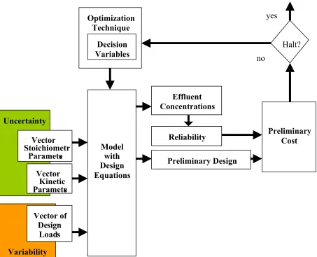
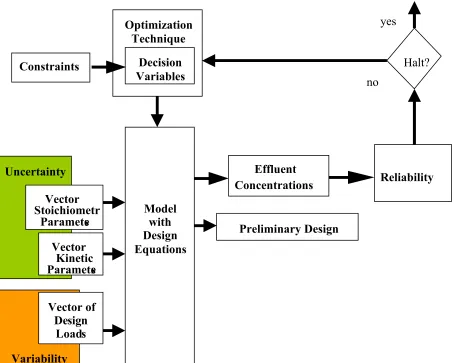
A third conceptual framework taking uncertainty and variability of inputs is

then presented for determining the reliability of a design. Reliability is defined as the

expectation that a design meets a given criterion over an operational period.

Finally, a fourth conceptual model is presented to show the tradeoff between

cost and reliability. This framework incorporates uncertainty and variability into the

design optimization process.

Before presenting the conceptual models, definitions of uncertainty,

variability, and reliability are presented. Chapter 2 provides a much longer discussion

of these concepts. The definitions presented here are specifically for wastewater

treatment design and the case study is used to illustrate the conceptual models.

Variability, as used here, corresponds to variance as used by others (Webster

and Mackay, 2003). Variability in data arises from heterogeneity that can be

quantified with a probability density function (PDF). Variability cannot be reduced

with additional research or knowledge. Sources of variability may be temporal,

behavioral, or weather-related (Bennett

et al.

, 1999; Huijbregts

et al.

, 2000). In the

data; behavioral data variability is due to population growth or decline, changes in

diet, changes in per capita water use, aging of the sanitary sewer system, industrial

change, and expansion of the sanitary sewer system; and weather-related variability is

due to rainfall and drought periods. All of these have different impacts on the

system’s performance. Mechanical and operational failures are other important

sources of variability in wastewater treatment system performance, but these are not

included within this analysis (Tchobanoglous

et al.

, 2003).

Uncertainty, unlike variability, can be reduced with additional research and

knowledge. Uncertainty, like variability, is generally characterized with a PDF and is

applicable to parameters used in modeling. Some model parameters are directly

measurable (such as oxygen concentrations in the influent or recycle wastewater), but

many are not. Instead, determination of the parameter values is indirect. A model is

used to predict how and why changes over time occur to certain observable values,

e.g., the oxygen, nitrogen, or other substrate concentration. Curve fitting techniques

are used in conjunction with the model for parameter determination. Uncertainty may

arise from many sources in such a process, such as measurements, of model structure

with lumped parameters, poorly defined models, or from lack of knowledge (Beck,

1982, 1984, 1989; Bennett

et al.

, 1999).

Reliability as used here is the percentage of time (or cases) in which the

design is expected to meet the effluent concentration limit. This is a definition in

agreement with others (Niku

et al.

, 1979; Tchobanoglous

et al.

, 2003).

Mathematically, this is:

300

,

7

1

v

where r is the reliability for one set of realizations using the variable loadings and

uncertain parameters; and v is the number of violations counted. 100 assessments are

performed whereupon the mean and standard deviation of the reliability is computed.

The expected reliability value reported is for

300

,

7

2

1













₊

_⋅

−

=

σ

v

R

(13)

where R is the reliability for 100 sets of realizations,

v

is the mean number of

effluent violations, σ is the standard error of the number of effluent violations, and

7,300 is the number of days in 20 years (the anticipated life of the project). For any

one design, four different reliabilities are assessed – for ammonia, nitrate, total

nitrogen, and total phosphorus. This provides a framework for assessing the

reliability of the least-cost design and conventional design.

The remainder of this chapter is devoted to presenting the traditional model,

the deterministic optimization model, and the optimization under variability and

uncertainty model along with their respective strengths and weaknesses. Finally, a

comparison of the model for optimizing under variability and uncertainty is compared

with the stochastic programming technique.

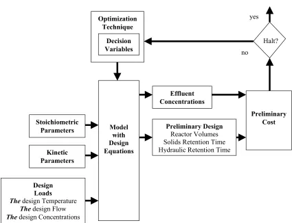
Traditional Design

Traditional design of wastewater treatment plants is typically a deterministic

process with inputs into a set of design equations that produce outputs as shown in

Figure 2.

Daily inputs

. These are the design loads of the system consisting of scalar

values for the design flows, the design temperature, and design influent

concentrations of various chemical species, e.g., biochemical oxygen demand (BOD),

chemical oxygen demand (COD), total Kjeldahl nitrogen (TKN), ammonia, etc.

Kinetic parameters

. Design equations are typically used requiring kinetic

parameter values or functions, e.g., the growth rate, the death or decay rate, reaction

rates, etc. The kinetic parameters required are model specific.

Stoichiometric parameters

. Stoichiometric parameters are the ratios of the

amounts of one chemical species required to react with another or to produce a

product. These are similar to kinetic parameters in that they are required in the design

equations, are model specific, and standard values are generally taken from the

literature. Neither stoichiometric nor kinetic values are constants. Constant values

are universal, e.g., g, c, π, e, etc. Parameter values are particular to the system being

Decision variables

. A set of decision variables is also typically used. Which

decision variables are required is model specific. Among the decision variables are

the recycle rates from one reactor to another, and the fraction of the reactor volume

that is unaerated (anoxic or anaerobic).

The model’s design equations are then used to generate outputs. These

outputs consist of

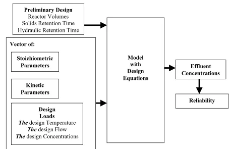
Preliminary design

. Among other features, the preliminary design consists

of the total reactor volumes, the hydraulic retention time (HRT), and the solids

retention time (SRT). HRT and SRT are the average time liquid and solid particles

spend in the wastewater treatment system, respectively. From the preliminary design,

calculation of the design cost can be performed.

Model with Design Equations Decision

Variables

Stoichiometric Parameters

Kinetic Parameters

Design Loads

The design Temperature

The design Flow

The design Concentrations

Effluent Concentrations

Preliminary Design

Reactor Volumes Solids Retention Time Hydraulic Retention Time

Preliminary Cost

Effluent concentrations

. The concentration of solids, BOD, ammonia,

nitrate, phosphate, etc. in the effluent can be determined. Generally, the design

engineer has a set of effluent limits that must be satisfied. If the design effluent

concentrations do not meet these required limits or the design is too expensive, then a

new set of decision variables is used and the process is repeated until the effluent

and/or cost limits are met.

One limitation of the traditional design approach is that there is no systematic

search of decision variable values for a least-cost design or for a high effluent quality

design. One means of addressing this is to use an optimization technique to perform a

search. This is addressed in the next section.

Halt?

Model with Design Equations Stoichiometric

Parameters

Kinetic Parameters

Design Loads

The design Temperature

The design Flow

The design Concentrations

Effluent Concentrations

Preliminary Design

Reactor Volumes Solids Retention Time Hydraulic Retention Time

Preliminary Cost Optimization

Technique

Decision Variables

yes

no

Deterministic Optimization Design

The deterministic optimization model is shown in Figure 3. There is much

similarity between the deterministic optimization model and the traditional model. In

both models, there are inputs of loadings, stoichiometric parameters, and kinetic

parameters. In both models, there are outputs of effluent concentrations and

preliminary designs. In both models, the design equations or activated sludge model

performing the design is the same.

There are differences, however, between the traditional design methodology

and the deterministic optimization methodology as a comparison of Figures 4 and 5

demonstrate. Among the differences are:

1.

An optimization technique is used to choose decision variable values

during the search procedure. The design problem is typically a

nonlinear (NLP) or mixed integer nonlinear programming (MINLP)

problem requiring an appropriate technique. During the search, the

decision variable values become part of the search. There may be

explicit limits on the search space of the decision variable values (e.g.,

non-negative values and/or upward limits).

2.

There may be a penalty assessed for exceeding the effluent limits in

searching for low-cost solutions. Care should be taken in the size of

the penalty. If the penalty is too large, it may drive the solution to a

more expensive solution than necessary. If the penalty is too small,

only infeasible solutions may be found. Choosing appropriate penalty

effluent limit violations is to have explicit effluent limit constraints in

the optimization procedure. In the traditional design approach, the

design engineer would reconfigure the plant typically by adjusting the

HRT or SRT (depending on the model) together with a new round of

calculations.

3.

There must be an explicit halting criterion such as little or no

improvement after a fixed number of iterations.

With both the traditional means of design and the optimized design procedure,

there is the question of what values should be used for the loads and the parameters.

This is also tied to the safety factor. The safety factor may be applied to the input, the

output, or some intermediate calculation within the model. One means of implicitly

applying the safety factor to the inputs is the statistical and “back of the envelope”

means of choosing design loads and perhaps in the choice of stoichiometric and

kinetic parameters from the literature. An explicit means of applying the safety factor

to the outputs is by increasing the size of the design volume by some factor or by

decreasing the allowed effluent limit from 5 mg BOD L

_{to 3 mg BOD L}

_{, for}

example. A problem with using the safety factor on the outputs is that it probably is

used in combination with a safety factor in choice of the inputs. This leads to an even

more conservative and possibly expensive design without necessarily providing a

worthwhile benefit. These input and output safety factor mechanisms contrast with

explicit safety factor values of 20-30 used in earlier design procedures for the HRT

when BOD

removal in conventional activated sludge systems (Eckenfelder, 1967;

Again, however, this explicit intermediate safety factor may unknowingly be

combined with an implicit design load safety factor leading to an even more

conservative design.

It has already been suggested that applying explicit safety factors to either

intermediate calculations or to outputs may be overly conservative because there may

also be an implicit safety factor built into the choice of design loads and parameter

values. Yet, might the choice of the design loads not also be overly conservative? If

statistical means are used to choose the design loads from historical data, there is no

way of knowing with any certainty which percentile of flow should be combined with

which percentile of waste concentration to provide a reliable, least-cost design.

Combining a flow between the 95

and 99

percentiles, with a low temperature, and

concentrations in the 95

to 99

percentile creates a design for a cold day with large

flow, COD, TKN, ammonia, etc. loads.

It is unlikely that such a cold day with extremely large flows of strong

wastewater will occur. Unusually large flows are most likely to occur due to rain.

Even in sewer systems with separate storm and sanitary sewers (as is typical in the

United States), rain has a large impact on the wastewater treatment plant (WWTP)

flow loading. This is because the sanitary sewers leak with groundwater infiltration

as the water table rises. In addition, when it rains, water flows into sanitary sewers

through manholes. The effect is that the wastewater is likely to be dilute (rather than

Rather than using a safety factor in design, another approach is assessing the

reliability of the preliminary design using a model. Figure 4 shows a schematic of a

reliability assessment procedure for a preliminary design, whether found using a

traditional design methodology or a deterministic optimization methodology. In this

procedure, the design characteristics of a preliminary design are used together with

vectors of loadings, kinetic parameters, and stoichiometric parameters. This raises

two important questions: 1) what size vectors should be supplied? and 2) what type of

model should be used in the analysis: steady state or dynamic? Typically, design is

carried out under steady state conditions even when a dynamic model is used (e.g.,

Rivas

et al.

, 2001) while simulation is carried out under dynamic conditions

(Rousseau

et al.

, 2001).

Model

with

Design

Equations

Effluent

Concentrations

Preliminary Design

Reactor Volumes

Solids Retention Time

Hydraulic Retention Time

Vector of:

Stoichiometric

Parameters

Kinetic

Parameters

Design

Loads

The

design Temperature

The

design Flow

The

design Concentrations

Reliability

The answers to the two questions above are closely interrelated. The size of

the vectors depends on two factors: the design life of the project and the time step the

model requires. With a dynamic model, the time steps are relatively small requiring

large vectors and making the process computationally intensive. The data available

often has a different time step than the dynamic model requires as well as gaps within

the data. This may lead the modeler to use the same data values repeatedly, the data

mixed with noise, or use a statistical methodology for generating data. Rather than

using a dynamic model, a steady-state model can be used. The advantages of the

steady-state model include fewer input requirements, smaller vectors for the same

project life, and less computational intensity. This is the approach used here.

The design loads may be based on historical information available (if such

information is available). This means that the relatively large variability in the design

loads can be characterized statistically and translated to uncertainty in future loadings.

It is worth noting that the amount of information available can be extended to longer

periods if the seasonality of the data is captured within the historical data available

(Wallace

et al.

, 1994).

Typically, there are no kinetic or stoichiometric data available for the specific

system to be designed. The only source of information available is from the literature

or from guidelines. As a result, there is uncertainty attached to the stoichiometric and

kinetic parameter values typically used in design. The designer does not know the

mean value and is even less sure of the distribution of the uncertainty in the parameter