DOI: 10.1534/genetics.107.085332
Note
Exploring Population Genetic Models With Recombination
Using Efficient Forward-Time Simulations
Badri Padhukasahasram,*
,1Paul Marjoram,
†Jeffrey D. Wall,
‡Carlos D. Bustamante* and Magnus Nordborg
§*Biological Statistics and Computational Biology, Cornell University, Ithaca, New York 14850,†Biostatistics Division, Department of Preventive Medicine, Keck School of Medicine, University of Southern California, Los Angeles, California 90089,‡Institute of Human Genetics, University of California, San Francisco, California 94143
and§Molecular and Computational Biology, University of Southern California, Los Angeles, California 90089
Manuscript received December 2, 2007 Accepted for publication January 26, 2008
ABSTRACT
We present an exact forward-in-time algorithm that can efficiently simulate the evolution of a finite population under the Wright–Fisher model. We used simulations based on this algorithm to verify the accuracy of the ancestral recombination graph approximation by comparing it to the exact Wright–Fisher scenario. We find that the recombination graph is generally a very good approximation for models with complete outcrossing, whereas, for models with self-fertilization, the approximation becomes slightly inexact for some combinations of selfing and recombination parameters.
C
OALESCENT theory provides a continuous-time approximation for the history of small samples in large populations and coalescent simulation is a widely used tool in population genetics. Under this framework, the genealogy of a sample of DNA sequences is modeled backward in time and neutral mutations are superposed on this genealogy to generate sequence polymorphism data (Kingman 1982; Hudson 1983; Rosenberg andNordborg 2002). Forward simulations, in contrast,
model the evolution of all the sequences in a population exactly, forward in time and generation by generation. Because coalescent simulations consider only those chro-mosomes that carry material ancestral to the sample, and, by making a continuous-time approximation skip uninteresting generations whose events do not affect the sample, they are computationally much more efficient than forward simulation programs. However, despite their inefficiency, forward simulations are necessary if we wish to simulate data sets under complex and realistic biological scenarios (e.g., natural selection at multiple linked loci) that are difficult to model accurately using the coalescent. Given the dramatic growth in the power of computing, forward-time simulations are currently feasible for large genomic regions (e.g., megabase scale) and many simulation packages have been developed
recently (e.g., Balloux2001; Hey2004; Hoggartet al.
2005; Peng and Kimmel 2005; Dudek et al. 2006;
Guillaume and Rougemont 2006; Sanford et al.
2007) and have also found important applications (e.g., Ballouxand Goudet2002; Pineda-Krchand Redfield
2005; Pengand Kimmel2007). Here, we present an exact
forward-in-time algorithm that can efficiently simulate the evolution of a finite population undergoing muta-tions, recombination, and natural selection at multiple linked loci. In contrast to existing forward-time simulators that consider the population genealogy generation by generation, our forward algorithm uses the genealogical information for multiple generations at a time, and on the basis of this information, simulates only those chromo-somes in the next generation that can potentially con-tribute to the future population. We show that such a forward–backward scheme combined with other optimi-zations can lead to substantial improvements in run-time efficiency. We use our simulation program to evaluate coalescent models with recombination by comparing them to the exact Wright–Fisher model.
SIMULATION ALGORITHM
Our algorithm is implemented in the C11 program-ming language and we simulate data sets under the Wright– Fisher model assumptions. Individuals in a population are assumed to be diploid, the population size is assumed 1Corresponding author:Biological Statistics and Computational Biology,
Room 169, Biotechnology Building, Cornell University, Ithaca, NY 14850. E-mail: [email protected]
constant (this assumption can readily be relaxed), and generations are always nonoverlapping. Chromosomes within the population are represented by sorted arrays of integers that correspond to the locations of their muta-tions in base pairs. In this representation, a location is considered polymorphic if it occurs in some but not all of the chromosomes. Over time, the chromosome arrays undergo changes due to recombination (i.e., are partially replaced by parts of other arrays) and mutation (i.e., new integer locations get inserted). They also increase or decrease in the number of copies due to genetic drift. At any given time, we keep track of chromosomes belong-ing only to the current and previous generations and keep reusing these arrays. We use a pseudo infinite-sites model for mutations (i.e., where the number of sites is finite but new mutations can appear only at non-polymorphic locations) and a finite-sites model for re-combination and remove locations that are no longer polymorphic, at regular intervals. The total number of new mutations added to a chromosome in any particular generation is modeled as a Poisson random variable with mean equal to the per-generation per-sequence muta-tion rateu. Meiotic recombination is modeled as a single crossing-over event and the probability that a recombi-nation event occurs in any particular generation is equal to 1 er, where r denotes the generation
per-sequence rate of recombination.Our forward algori-thm proceeds by simulating the population in the next generation as a function of (i) the population in the previous generation and (ii) the simulated genealogy for the next k generations. We use the simulated ge-nealogy to tell us which of the chromosomes in the next generation can contribute material to the future pop-ulation that exists afterkgenerations from now. Only
those chromosomes are explicitly simulated in the next generation since all the other chromosomes are des-tined to disappear. We outline all the steps in our simulation program below:
1. Let gen(0) represent the current generation, gen(1) represent the generation being simulated, and gen(2), gen(3), gen(4), . . ., etc., represent subsequent gen-erations. Before creating the individuals of gen(1), we generate the future genealogical information of the population for k generations ½i.e., information re-quired for creating gen(2) to gen(k11). This involves simulating the ancestry of the chromosomes in the nextkgenerations and determining whether or not they will undergo recombination in any particular gen-eration. Using this information, we can see that two key events are possible:
a. All the descendants of a chromosome belong-ing to gen(1) may be lost by gen(k11) with-out any of their homologs having undergone recombination.
b. A chromosome or its homolog may recombine in gen(2), but both of them can lose all their descendants by gen(k11) without any of their homologs having undergone any subsequent recombination½i.e., from gen(3) to gen(k11). Chromosomes that belong to categoriesaorb, cannot potentially leave any trace in the future population that exists at gen(k11). Therefore, it is not necessary to explicitly simulate such chromosomes in gen(1).
2. Chromosomes of gen(1) are created by randomly sampling chromosomes from gen(0) and determin-ing whether or not they undergo recombination. When a chromosome of gen(0) gets chosen the first time and does not recombine, we simply exchange the pointers to the arrays between gen(1) and gen(0) to create a new chromosome of gen(1). If it gets picked again or if it undergoes recombination, we create a new chromosome by copying parts of the relevant arrays into the arrays of gen(1) using the memcpy() function. The only exception to this occurs when a recombination is the last event in-volving a particular individual. In this case, we first exchange the pointers to the arrays for one of the homologs (provided it has not been picked already) and explicitly copy only part of the other array using memcpy(). After creating all the chromosomes of gen(1), we generate new mutation locations for each chromosome and insert them into the sorted arrays using a binary search and the memove() function. 3. Using the future genealogical information, create
only those chromosomes in gen(1) that can poten-tially contribute to the population that exists at gen (k11). Assume that the other arrays are empty.½Note that the main idea in step 2, when creating a new generation, was to reuse the arrays from the previous
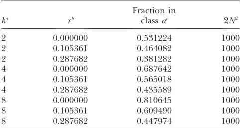
TABLE 1
The fraction of chromosomes in classaas a function ofkandr
ka rb
Fraction in
classac 2Nd
2 0.000000 0.531224 1000
2 0.105361 0.464082 1000
2 0.287682 0.381282 1000
4 0.000000 0.687642 1000
4 0.105361 0.565018 1000
4 0.287682 0.435589 1000
8 0.000000 0.810645 1000
8 0.105361 0.609490 1000
8 0.287682 0.447974 1000
aNumber of generations of look-ahead under the standard
neutral model. b
Per-generation per-sequence recombination rate. c
Average fraction of chromosomes in classaas determined from 10 million simulations. Chromosomes in classacannot potentially leave any trace in the future population that exists afterkgenerations.
d
generation as much as possible and avoid copying. If we eliminate some of the nonancestral chromosomes from any generation (seeappendix a), the fraction
of chromosomes for which explicit array copying is necessary decreases substantially.
4. Update the future genealogy by one more genera-tion. Repeat step 3. Remove nonpolymorphic loca-tions from the population at regular intervals. 5. Simulate the whole population during the lastk1 2
generations of the simulation (i.e., if the simulation is run forlgenerations, we explicitly simulate all the chromosomes from generationslk1 tol) as well as during the lastk12 generations up to the generation during which nonpolymorphic locations get removed from the population (i.e., if fixed mutations get removed every n generations, then we explicitly simulate all the chromosomes from generationsn
k1 ton, 2nk1 to 2n, 3nk1 to 3n,. . ., etc.). ½Note that this last step is essential because at the end of the simulation as well as during the generation at which nonpolymorphic locations get removed, we
require all the chromosomes present in the popula-tion (for example, to determine which chromosomal locations are nonpolymorphic) and not just the ones that can contribute to the future population.
The parameterkhas to be chosen optimally for this algorithm to work most effectively. There is a trade-off between the computational effort spent to look forward forkgenerations and the effort saved by the elimination of nonancestral chromosomes from the next genera-tion. In terms of run-time complexity, creating a new generation mainly involves array copy operations that take linear ½i.e.,O(N)time in terms of the number of mutations ½binary search takes O(ln(N)) time while exchanging the pointers takes constant time accumu-lated in the array. In contrast, looking forward for a few generations takes only constant time and is indepen-dent of the number of mutations carried.
The expected proportion of individuals in categoriesa
orbfirst increases as the depth of the look-ahead (i.e.,k) increases but eventually becomes nearly constant. So,
TABLE 2
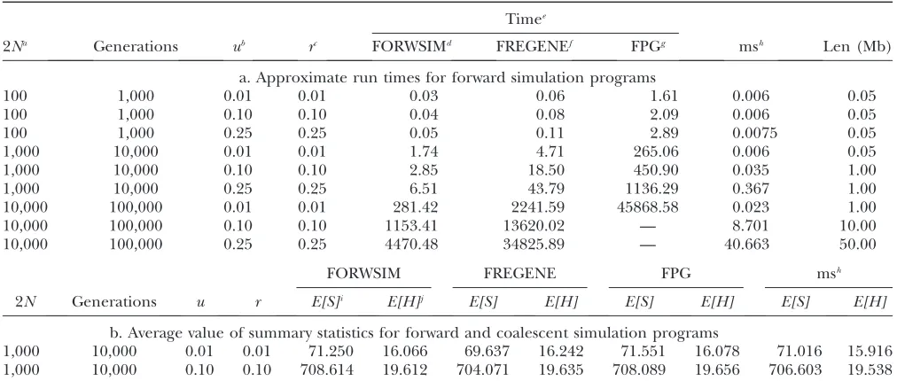
Approximate run times for forward simulation programs and average value of summary statistics for forward and coalescent simulation programs
Timee
2Na Generations ub rc FORWSIMd FREGENEf FPGg msh Len (Mb)
a. Approximate run times for forward simulation programs
100 1,000 0.01 0.01 0.03 0.06 1.61 0.006 0.05
100 1,000 0.10 0.10 0.04 0.08 2.09 0.006 0.05
100 1,000 0.25 0.25 0.05 0.11 2.89 0.0075 0.05
1,000 10,000 0.01 0.01 1.74 4.71 265.06 0.006 0.05
1,000 10,000 0.10 0.10 2.85 18.50 450.90 0.035 1.00
1,000 10,000 0.25 0.25 6.51 43.79 1136.29 0.367 1.00
10,000 100,000 0.01 0.01 281.42 2241.59 45868.58 0.023 1.00
10,000 100,000 0.10 0.10 1153.41 13620.02 — 8.701 10.00
10,000 100,000 0.25 0.25 4470.48 34825.89 — 40.663 50.00
FORWSIM FREGENE FPG msh
2N Generations u r E[S]i E[H]j E[S] E[H] E[S] E[H] E[S] E[H]
b. Average value of summary statistics for forward and coalescent simulation programs
1,000 10,000 0.01 0.01 71.250 16.066 69.637 16.242 71.551 16.078 71.016 15.916 1,000 10,000 0.10 0.10 708.614 19.612 704.071 19.635 708.089 19.656 706.603 19.538
aTotal number of chromosomes under the standard neutral Wright–Fisher model with constant population size and with
uni-form mutation and recombination rates. bPer-generation per-sequence mutation rate.
cPer-generation per-sequence recombination rate.
dFORWSIM is our C11program freely available at http://people.cornell.edu/pages/bp85. e
Time taken in seconds for a single run on a 2.2 Ghz 64-bit AMD processor machine with 8 GB of RAM. f
FREGENE is a C11program freely available at http://www.ebi.ac.uk/projects/BARGEN/download/FREGEN/fregeneweb.html. g
FPG is a C program freely available at http://lifesci.rutgers.edu/heylab/ProgramsandData/Programs/FPG/FPG_Documentation. htm#FilesinthisPackage. For FPG, the number of chromosome segments was always fixed at 500.
h
ms is a C program that simulates data sets under the coalescent framework and is freely available at http://home.uchicago.edu/ rhudson1/source.html. ms was run with population crossing-over rater¼4Nrand population mutation rateu¼4Nuand sample size of 20. (For details about ms, see Hudson2002.)
i
Total number of SNPs for a sample size of 20 chromosomes. Average values are based on 1000 simulations. j
increasingkbeyond a certain range will not be desirable. The expected proportion decreases as the per-generation per-sequence recombination rate increases, and there-fore this strategy becomes less effective for high values of r. Table 1 shows the expectation of the fraction of chromosomes in categoryaas a function ofkandrfor a population with 500 diploid individuals and evolving under the standard neutral model (also seeappendix a).
In all the simulations presented here, we use a fixed value of k¼ 8 and remove nonpolymorphic locations after everyN generations, where N denotes the size of the population (appendix bshows some run-time
com-parisons for different values of the look-ahead parameter). For models with natural selection, we simulate the evolution of selected and neutral sites separately. We first generate the future genealogical information by simulating the ancestry of all the chromosomes in the population considering only the selected sites. If the number of sites under selection remains small, this in-formation can be generated quickly. Then, using this information, we simulate the evolution of the remaining (neutral) sites according to the algorithm described earlier. Note that as the proportion of sites under selec-tion increases, the look-ahead strategy becomes relatively less effective.
Random number generation: Random numbers are generated using the Mersenne Twister algorithm
(Matsumotoand Nishimura1998). The external files
mtrand.cpp and mtrand.h are used along with our pro-gram to enable random number generation. mtrand.cpp is a fast and high-quality random number generator whose period length is a large prime number that is one less than a power of 2.
Comparison with other forward simulation pro-grams: We first compare the approximate running time of our simulation program (FORWSIM) with two other currently available forward-time simulation programs for the standard neutral model. These comparisons demon-strate that our look-ahead demon-strategy combined with other standard optimizations can result in large gains in run-time efficiency (Table 2a,appendix cshows some
run-time comparisons for models with natural selection at multiple sites). The comparisons also confirmed that, for all the programs tested, the means and distributions of some simple summary statistics are in agreement with coalescent simulations (Table 2b, Figure 1).
IS THE ANCESTRAL RECOMBINATION GRAPH A GOOD APPROXIMATION
TO THE EXACT SCENARIO?
Under the coalescent framework, the genealogy of a sample of sequences with recombination can be approx-imated by a graph called the ancestral recombination
graph (ARG) (e.g., see Hudson 1983; Griffiths and
Marjoram 1996). If s denotes the probability of
self-fertilization andF¼s/(2s), the genealogy of a sample for partial selfing (i.e., 0,s,1) can be approximated by an outcrossing version of the ARG with a rate of coa-lescence that is 11Ftimes faster and a rate of recom-bination that is 1stimes slower (see Nordborg2000).
The recombination graph makes two main assumptions:
1. It assumes that the lineages we follow backward in time recombine only with nonancestral lineages. This follows because we are tracing the ancestry of small samples in large populations and therefore the number of lineages ancestral to the sample remains small compared to the total population size.
2. It also assumes that in a large population all the re-combination events are independent of one another. We use forward simulations of the exact Wright– Fisher model with and without self-fertilization and compare the expected decay of pairwise linkage disequilibrium (LD) to values generated with equiv-alent coalescent simulations and verify the accuracy of these approximations.
When the recombination rate is high, the number of ancestral lineages in the recombination graph can be-come very large and so it is not obvious whether the first approximation will be accurate in finite populations. When there is partial selfing, going backward in time, a
pair of lineages resulting from a single recombination event can spend a significant amount of time together within the same ancestors before they find different parents or coalesce. Thus, it can be shown that there is a significant probability that such lineages may recom-bine again (i.e., overlapping recombinations) before they find different ancestors (see appendix d, Figure
2a). This clearly violates the assumption that all recom-bination events happen independently of one another. For models without selfing, the probability of such over-lapping recombination events is expected to be much smaller as long as the population size is reasonably large (seeappendix d, Figure 2b).
Figure 3 shows the expected decay of the absolute value of pairwiseD9(the normalized measure of LD that takes values between1 and 1) for forward-time simulations with selfing, forward-time simulations without selfing, and coalescent simulations with equivalent parameters. When simulating using the coalescent, we assume that recombination happens only with nonancestral chromo-somes, which ignores the chance of recombination events between ancestral lineages. Whenris high, the expected value of D9 is slightly higher in forward simulations without selfing than in comparable coalescent simula-tions presumably because the number of ancestral line-ages is large and recombinations with ancestral lineline-ages are not rare. Because recombination events with ancestral lineages will be associated with some coalescence, we
reach the most recent common ancestor slightly sooner in the exact case than in the ARG. Nevertheless, for models with only outcrossing, we see from results in Figures 1, 3, and from Table 2, that the expectations and distributions under the coalescent with recombination are close to the expectations under the exact scenario even for higher values ofr. We also compared the frequencies of some triplet based LD patterns (Padhukasahasramet al.2004,
2006) at different distances and reached similar conclu-sions (results not shown here). For models with selfing, the ARG remains a close approximation to reality as long as eitherrorsremains small (Figures 3 and 4, Table 3). Whenrandsare both very high, the ARG approximation breaks down due to overlapping recombination events and expected value ofD9is significantly higher in forward simulations compared to the equivalent coalescent model.
Figure3.—(a) The expected decay of pairwise
D9for coalescent simulations withr¼2.0 andu¼ 51.0 (shaded curve), forward simulations withr¼ 0.001,u¼0.0255, and 2N¼1000 (solid dashed curve), and forward simulations with selfing for
r¼0.05,u¼0.05, 2N¼1000, ands¼0.98 (solid curve). (b) The expected decay of pairwiseD9for coalescent simulations withr¼20.0 andu¼51.0 (shaded curve), forward simulations withr¼0.01,
u¼0.0255, and 2N¼1000 (solid dashed curve), forward simulations withr¼0.5,u¼0.05, 2N¼ 1000, ands¼0.98 ( solid curve), and forward sim-ulations withr¼0.05,u¼0.005, 2N¼10,000, and
SUMMARY
We have presented an exact forward-in-time algo-rithm that can efficiently simulate the evolution of a
finite population under the Wright–Fisher model of evolution. Comparisons with other currently available forward-in-time simulators show that our C11program is able to simulate data sets quickly and all the tested
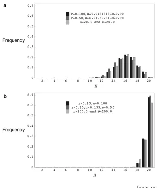
Figure4.—(a) The distribution of the number of distinct haplotypes H for coalescent simula-tions withr¼20.0 andu¼20.0, forward simula-tions withr¼0.100,u¼0.0181818,s¼0.90, and 2N¼1000 and forward simulations withr¼0.50,
u¼0.01960784,s¼0.98, and 2N¼1000. (b) The distribution of the number of distinct haplotypes
Hfor coalescent simulations withr¼200.0 and u¼200.0, forward simulations withr¼0.200,u¼ 0.1333333,s¼0.50, and 2N¼1000 and forward simulations withr ¼ 0.10, u¼ 0.10, and 2N ¼ 1000. H values are for samples of 20 chromo-somes drawn from the final population and for-ward simulation programs were run for 40N
generations for models with selfing and 20N gen-erations for models without selfing.
TABLE 3
Average value of summary statistics for forward simulations with and without selfing
FORWSIMe msf
2Na Generations ub rc sd E[S]g E[H]h E[S] E[H]
1,000 10,000 0.0100 0.0100 0.00 71.250 16.066 71.016 15.916
1,000 20,000 0.0182 0.1000 0.90 70.687 15.968 71.016 15.916
1,000 20,000 0.0196 0.5000 0.98 70.804 15.586 71.016 15.916
1,000 10,000 0.1000 0.1000 0.00 708.614 19.612 706.603 19.538
1,000 20,000 0.1333 0.2000 0.50 711.662 19.563 706.603 19.538
a
Total number of chromosomes under the standard neutral Wright–Fisher model with constant population size and uniform mutation and recombination rates.
b
Per-generation per-sequence mutation rate. c
Per-generation per-sequence recombination rate. d
Probability of selfing. e
FORWSIM is our forward simulation program written in C11 and is freely available at http://people. cornell.edu/pages/bp85.
f
ms is a C program that simulates data sets under the coalescent framework and is freely available at http:// home.uchicago.edu/rhudson1/source.html. ms was run with the population crossing-over rater¼4Nrand population mutation rateu¼4Nu.
gTotal number of SNPs for a sample size of 20 chromosomes. Average values are based on 1000 simulations.
hNumber of distinct haplotypes. Average values are based on a sample of 20 chromosomes and 1000
programs appear to function correctly. Further refine-ments to our algorithm are possible to improve its ef-ficiency. For example, instead of using a constant depth of look-ahead, we may change the depth during the run. Note that toward the later stages of a simulation, when the amount of polymorphism in the population becomes high, a deeper look-ahead might prove to be more advantageous. Also, it may be possible to de-termine other categories of chromosomes (apart from those in classesaorb) that cannot potentially leave any trace in the future population that exists after k gen-erations. Alternately, instead of using the look-ahead strategy described before, we may explicitly construct chromosomes for a small number of generations in terms of the chromosomes of gen(1) by generating the recombination breakpoints of the future (this may be useful whenris very high). Doing this will allow us to eliminate all the chromosomes that are nonancestral to the population that exists at gen(k11) but will require greater computational effort than the former look-ahead strategy. Finally, we anticipate that a parallel im-plementation of this algorithm that can simultaneously utilize a large number of computer processors (which can all access the same memory), can make forward-time simulations practical for very large populations.
We checked the accuracy of the ancestral recombina-tion graph approximarecombina-tion by comparing the expected decay of pairwise linkage disequilibrium in forward and coalescent simulations. Our results indicate that the standard coalescent with recombination will be a close approximation to the exact scenario for completely out-crossing populations with 2N¼1000 chromosomes or more, even for higher values ofr. The ARG is also a good approximation for models with selfing as long as either the selfing rate (s) or recombination rate (r) remains small. Whensandrare both very high, the scaled ARG for partial self-fertilization becomes slightly inexact due to substantial probability of overlapping recombination events. Therefore, for such parameter ranges, it is best to simulate data sets using exact Wright–Fisher simulations (or alternately modify existing coalescent simulation pro-grams to allow for overlapping recombination events).
We thank Andrew G. Clark and members of the Bustamante lab for providing comments on this project. This work was supported by National Science Foundation grant DBI-0606461 to Susan McCouch and Carlos D. Bustamante as well as by National Institutes of Health (NIH), Center for Excellence in Genomic Sciences grants HG-002790 and GM-069890 to Paul Marjoram and Magnus Nordborg. This work
was also supported in part by NIH grant R01-HG004049-02 to Jeffrey D. Wall, Paul Marjoram, and Magnus Nordborg.
LITERATURE CITED
Balloux, F., 2001 EASYPOP (Version 1.7): a computer program for
population genetics simulation. J. Hered.92:301–302.
Balloux, F., and J. Goudet, 2002 Statistical properties of
popula-tion differentiapopula-tion estimators under stepwise mutapopula-tion in a
fi-nite island model. Mol. Ecol.11:771–783.
Dudek, S. M., A. A. Motsinger, D. R. Velez, S. M. Williamsand
M. D. Ritchie, 2006 Data simulation software for whole-genome
association and other studies in human genetics. Pac. Sym.
Bio-comput.11:499–510
Griffiths, R. C., and P. Marjoram, 1996 Ancestral inference from
samples of DNA sequences with recombination. J. Comput. Biol.
3:479–502.
Guillaume, F., and J. Rougemont, 2006 Nemo: an evolutionary
and population genetics programming framework.
Bioinfor-matics22:2556–2557.
Hey, J., 2004 FPG: A computer program for forward population
ge-netic simulation. http://lifesci.rutgers.edu/heylab/HeylabSoftware. htm#FPG.
Hoggart, C., T. G. Clark, R. Lampariello, M. De Iorio, J.
Whittakeret al., 2005 FREGENE: software for simulating large
genomic regions. Technical Report. Department of Epidemiology and Public Health, Imperial College, London.
Hudson, R. R., 1983 Properties of a neutral allele model with
intra-genic recombination. Theor. Popul. Biol.23:183–201.
Hudson, R. R., 2002 Generating samples under a Wright–Fisher
neutral model of genetic variation. Bioinformatics18:337–338.
Kingman, J. F. C., 1982 The coalescent. Stochast. Proc. Appl.13:
235–248.
Matsumoto, M., and T. Nishimura, 1998 Mersenne Twister: a 623
dimensionally equidistributed uniform pseudorandom number
generator. ACM Trans. Model. Comput. Simul.8:3–30.
Nordborg, M., 2000 Linkage disequilibrium, gene trees, and
self-ing: an ancestral recombination graph with partial self-fertiliza-tion. Genetics154:923–929.
Padhukasahasram, B., P. Marjoram and M. Nordborg,
2004 Estimating the rate of gene-conversion on human
chro-mosome 21. Am. J. Hum. Genet.75:386–397.
Padhukasahasram, B., J. D. Wall, P. Marjoramand M. Nordborg,
2006 Estimating recombination rates from single-nucleotide
polymorphisms using summary statistics. Genetics174:1517–1528.
Peng, B., and M. Kimmel, 2005 simuPOP: a forward-time population
genetics simulation environment. Bioinformatics21:3686–3687.
Peng, B., and M. Kimmel, 2007 Simulations provide support for the
com-mon disease–comcom-mon variant hypothesis. Genetics175:763–776.
Pineda-Krch, M., and R. J. Redfield, 2005 Persistence and loss of
meiotic recombination hotspots. Genetics169:2319–2333.
Rosenberg, N. A., and M. Nordborg, 2002 Genealogical trees,
co-alescent theory and the analysis of genetic polymorphisms. Nat.
Rev. Genet.3:380–390.
Sanford, J., J. Baumgardner, W. Brewer, P. Gibsonand W. ReMine,
2007 Mendel’s accountant: a biologically realistic forward-time
population genetics program. Scalable Computing: Practice and
Experience.8:147–165
APPENDIX A: CALCULATIONS
Let gen(0) represent the current generation, gen(1) represent the generation being simulated and gen(2), gen(3), gen(4), . . ., etc., represent subsequent generations. Let 2N denote the total number of chromosomes in the population andkdenote the number of generations of look-ahead. Assuming random mating as follows:v(m), the probability thatmchromosomes do not get chosen for the next generation is (1m/2N)2N;q(m), the probability that a
chromosome is chosen exactlymtimes is2NC
m(1/2N)m(11/2N)2Nm.
Assumingncopies of a chromosome in the current generation, the probability that exactlymcopies get chosen in the next generation iss(n,m)¼2NC
m(n/2N)m(1n/2N)2Nm.
The chance that a chromosome does not recombine in any given generation is approximatelyer.
Assuming n copies of a chromosome in the current generation, the chance that none of the copies of the chromosome that get picked in the next generation, recombine, can be approximated as
plðn;rÞ ¼sðn;0Þ1sðn;1Þer1sðn; 2Þe2r . . .sðn;lÞelr; ðA1Þ whereldenotes the maximum number of copies that can be picked in the next generation.
Fork¼1 andr.0, a chromosome can be lost if it does not get picked in gen(2). Therefore, the chance that a chromosome is lost without its homolog having undergone recombination is
qð0Þp2Nð1;rÞ:
Fork¼2 andr.0, a chromosome can be lost if it does not get picked in gen(2) or gets picked 1 to 2N1 times in gen(2) but none of those copies get picked in gen(3). Therefore, the probability that all the copies of a chromosome are lost without any of their homologs having undergone any recombination is nearly
qð0Þp2Nð1; rÞ1½qð1Þvð1Þp2N1ð1;rÞp2Nð1;rÞ1 . . .qð2N 1Þvð2N 1Þp1ð1;rÞp2Nð2N 1;rÞ: ðA2Þ Note that if a chromosome gets pickedmtimes in the next generation, then its homolog can get picked at most 2Nm
times and therefore we have to chooselappropriately in the terms in Equation A2. We assume that if there arexcopies of a chromosome in any given generation, then there are alsox homologs, when calculating the probability that
FigureA1.—The fraction of chromosomes in category a as a function of recombination rate (r) and number of generations of look-ahead (k).
none of those homologs will recombine. There is a small chance that some of the copies of a chromosome will be homologs of one another in the next generation. Therefore, the probability given by Equation A2 is not exact.
In general, whenNis large,ais small andr.0, the chanceP(a) that all the descendants of a chromosome from gen(1) are lost at gen(a12) but not before that, without any of their homologs having undergone recombination is nearly Psð1;m1Þp2Nm1ð1;rÞsðm1;m2Þp2Nm2ðm1;rÞ. . .sðma1;maÞp2Nmaðma1;rÞsðma;0Þp2Nðma;rÞ, where m1,
m2,. . .,macan all vary from 1 to 2N 1. Therefore, fork. 0, the total probabilityT(k) that all the copies of a
chromosome are lost by gen(k11), without any of their homologs having undergone any recombination is nearly
sð1;0Þp2Nð1;rÞ1XPðaÞ; ðA3Þ whereavaries from 0 tok1. Table A1 shows the approximate probability given by (A3) as a function ofkandr. Figures A1 and A2 show different views of this likelihood surface.
Forr¼0,T(k) is exactly equal to
sð1;0Þ1 XUðaÞ; ðA4Þ
whereavaries from 0 tok1 andU(a)¼Psð1;m1Þsðm1;m2Þ. . .sðma1;maÞsðma;0Þ, wherem1,m2,. . .,maall vary
from 1 to 2N1.
APPENDIX B
TABLE A1
Approximate probability that a chromosome is in classaas calculated from Equation A3
ka rb Fraction in classac Fraction in classad 2Ne
2 0.000000 0.531224 0.531224 1000
2 0.105361 0.464134 0.464082 1000
2 0.287682 0.381373 0.381282 1000
4 0.000000 0.687639 0.687642 1000
4 0.105361 0.565068 0.565018 1000
4 0.287682 0.435686 0.435589 1000
8 0.000000 0.810644 0.810645 1000
8 0.105361 0.609553 0.609490 1000
8 0.287682 0.448077 0.447974 1000
a
Number of generations of look-ahead under the standard neutral model. b
Per-generation per-sequence recombination rate. c
Approximate probability that a chromosome is in classaas calculated from Equation A3. d
Probability that a chromosome is in classaas calculated from 10 million simulations. eTotal number of chromosomes in the diploid population.
TABLE B1
FORWSIM running times for different values of the look-ahead parameter
Timed
2Na Gen Length (Mb) ub rc No look-ahead ke¼2 k¼8 k¼12
10,000 100,000 1.0 0.01 0.01 381.35 210.73 170.28 198.59
10,000 100,000 20.0 0.10 0.10 2593.21 1082.32 771.02 786.98
10,000 100,000 50.0 0.25 0.05 6482.35 2329.72 1187.71 1151.42
10,000 100,000 50.0 0.25 0.25 7521.44 3546.32 2700.23 3006.86
20,000 200,000 20.0 0.01 0.01 2368.04 1192.49 915.21 1141.35
20,000 200,000 50.0 0.10 0.10 9505.73 3573.17 2192.54 2315.15
a
Total number of chromosomes in the diploid population. b
Per-generation per-sequence mutation rate. c
Per-generation per-sequence recombination rate. d
Time taken in seconds on a machine with two 2.66 GHz dual-core Intel Xeon processors and 8 GB of RAM. e
APPENDIX C
APPENDIX D
LetN be the total number of individuals in the population ands be the selfing probability and r be the per-generation per-sequence recombination rate. For a given chromosome, the chance of no recombination events in any given generation can be approximated byer. We first calculate the probability that, going backwards in time, a pair of
lineages resulting from a recombination event will eventually find two different ancestors.
The probability that it finds different ancestors in the first generation is (1s)(11/N) (i.e., not created by selfing and choose different ancestors).
The probability that it finds different ancestors in the second generation is (s/21(1s)/(2N))(1s)(11/N) ½i.e., probability of selfing but choosing different chromosomes in the same ancestor in the first generation (i.e.,s/2) or not created by selfing but picking different chromosomes within the same parent in the first generation (i.e., (1s)/ 2N) and then not created by selfing and choosing different ancestors in the second generation.
The probability that it finds different ancestors in the second generation without further recombination is (s/21(1s)/ (2N))(1s)(11/N)e2r.
In general, the probability that a pair finds different ancestors in the nth generation but not before that is: (s/21 (1s)/(2N))n1(1s)(11/N) and the probability that this happens without subsequent recombinations is (s/21
(1s)/(2N))n1(1s)(11/N)e(2n2)r.
Thus, the total probability that a recombination event will eventually split lineages into two separate ancestors is (summing up ton¼infinity) 2(1s)(11/N)/(2(s1(1s)/(N))). Now, the total probability that this happens without any subsequent recombination events is (summing appropriate terms up ton¼infinity) 2(1s)(11/N)/ (2 (s 1 (1 s)/(N))e2r
). Therefore, the probability of overlapping recombination events, given that after a recombination event the pair of lineages will find different ancestors is (s1(1s)/(N))(1e2r
)/(2(s1(1s)/
(N))e2r
). Figure 2a shows this probability as a function ofsandr.
Similarly, for models without self-fertilization, going backward in time, the probability that a pair of lineages finds different ancestors in the first generation is (11/N). The probability of finding different ancestors in the second generation is (11/N)/2N(i.e., pick different chromosomes in the same parent in the first generation (i.e., 1/2N) and pick different parents in the second generation, etc.). The probability of finding different ancestors in the second generation without subsequent recombination is (11/N)e2r
/2N.
In general, the probability that a pair of lineages finds different ancestors in the nth generation is (11/N)/
(2N)n1and the probability that this happens without subsequent recombinations is
ð11=NÞeð2n2Þr=ð2NÞn1:
The total probability that after a recombination event, a pair of lineages will eventually find two separate ancestors is (summing appropriate terms up to infinity) 2N2/(2N1) and the total probability that this happens without any subsequent recombination is 2N2/(2Ne2r). Therefore, the probability of overlapping recombination events,
given that a pair of lineages will eventually find two different individuals is: (1e2r)/(2
Ne2r). Figure 2b shows this
probability as a function ofNandr.
TABLE C1
Approximate run-times for models with positive selection at multiple sites
Timef
2Na Generations ub rc hd se NEWSELg FPGh
1,000 10,000 0.01 0.01 0.50 0.01 4.78 82.06
1,000 10,000 0.10 0.10 0.50 0.01 5.70 174.91
aTotal number of chromosomes under the standard Wright–Fisher model with constant population size and uniform mutation
and recombination rates.
bPer-generation per-sequence mutation rate.
cPer-generation per-sequence recombination rate.
dDominance. A value of 0.5 denotes incomplete dominance in heterozygotes.
eStrength of selection per sequence.
fApproximate time taken for a single run on a machine with two 2.66 GHz dual-core Intel Xeon processors and 8 GB of RAM.
gNEWSEL is our C11program freely available at http://people.cornell.edu/pages/bp85. We ran our simulation program un-der a simple model where 40 known sites are subject to positive selection and fitness effects are additive.
h