DOI: 10.1534/genetics.106.061317
Inference of Population Structure Under a Dirichlet Process Model
John P. Huelsenbeck*
,1and Peter Andolfatto
†*Department of Integrative Biology, University of California, Berkeley, California 94720 and†Section of Ecology, Behavior and Evolution, Division of Biological Sciences, University of California, San Diego, California 92093-0116
Manuscript received May 25, 2006 Accepted for publication December 24, 2006
ABSTRACT
Inferring population structure from genetic data sampled from some number of individuals is a for-midable statistical problem. One widely used approach considers the number of populations to be fixed and calculates the posterior probability of assigning individuals to each population. More recently, the assignment of individuals to populations and the number of populations have both been considered random variables that follow a Dirichlet process prior. We examined the statistical behavior of assignment of individuals to populations under a Dirichlet process prior. First, we examined a best-case scenario, in which all of the assumptions of the Dirichlet process prior were satisfied, by generating data under a Dirichlet process prior. Second, we examined the performance of the method when the genetic data were generated under a population genetics model with symmetric migration between populations. We examined the accuracy of population assignment using a distance on partitions. The method can be quite accurate with a moderate number of loci. As expected, inferences on the number of populations are more accurate when u ¼ 4Neu is large and when the migration rate (4Nem) is low. We also examined the sensitivity of inferences of population structure to choice of the parameter of the Dirichlet process model. Although inferences could be sensitive to the choice of the prior on the number of populations, this sensitivity occurred when the number of loci sampled was small; inferences are more robust to the prior on the number of populations when the number of sampled loci is large. Finally, we discuss several methods for summarizing the results of a Bayesian Markov chain Monte Carlo (MCMC) analysis of population structure. We develop the notion of the mean population partition, which is the partition of individuals to populations that minimizes the squared partition distance to the partitions sampled by the MCMC algorithm.
M
OST natural populations display some degree of population subdivision, either because they oc-cupy a large geographic area and cannot act as a single randomly mating population or because geographical barriers reduce migration between different areas. The consequence is that subpopulations from different geo-graphic regions occupied by a species show different allele frequencies. Population subdivision has pro-foundly important effects on the dynamics of alleles in populations and also on the statistical tests we might apply to genetic data sampled from individuals. It is well known that population subdivision affects the dynamics of alleles in a population under the influence of muta-tion, drift, and selection; hence, the eventual fate of an allele is affected by population subdivision (Wright1940, 1943). Moreover, undetected population sub-division has an important (and usually negative) effect on statistical tests that are commonly applied to ge-netic data sampled from populations. For example, sta-tistical tests of the presence of natural selection are
adversely affected by undetected population subdivi-sion, often having an inflated incidence of false posi-tives (Andolfatto and Przeworski 2000; Nielsen
2001; Przeworski 2002; Hammeret al.2003).
How can one identify the presence of population structure on the basis of genetic data sampled from some number of individuals? This is a long-standing problem in population genetics and has inspired a variety of approaches. One approach—F-statistics, developed by Wright(1951) and Male´ cot (1948)—
attempts to characterize the effect of population sub-division by its inbreeding-like effect on excess homozy-gosity. These approaches can be quite sophisticated
(e.g., Holsingeret al. 2002), but ultimately attempt to
characterize the potentially complex pattern of popu-lation subdivision with a single statistic;FST provides a
rather blunt tool for exploring population subdivision, with many different patterns of population subdivision, for example, producing a similar (positive)FST. Moreover,
these approaches rely on preexisting labels; the assign-ment of individuals to populations is considered to be known before the analysis of the genetic data begins.
More recently, several authors have developed meth-ods that do not rely upon a known assignment of 1Corresponding author: Section of Ecology, Behavior and Evolution,
Division of Biological Sciences, University of California, La Jolla, CA 92093-0116. E-mail: [email protected]
individuals to populations, instead inferring the pop-ulation structure. Perhaps the most widely used method is a Bayesian one developed by Pritchardet al. (2000).
In its simplest form, the method of Pritchard et al.
(2000) considers a fixed number of populations and, assuming linkage equilibrium and Hardy–Weinberg equilibrium of the alleles at the sampled loci, calculates the probability of assigning individuals to each of the populations. In its more fully developed form, the method has been modified to allow for admixture of individuals and linkage of the loci (Pritchard et al.
2000; Falushet al. 2003). Pritchardet al. (2000) use a
variant of Markov chain Monte Carlo (MCMC) to approximate the probabilities of assigning individuals to populations. The Bayesian method of Pritchard
et al. (2000) has the advantage that the uncertainty in the assignment of individuals to populations is easy to characterize. The method has also been of great practical importance, with uses in conservation genetics
(Moodleyand Harley2005; Smallet al. 2006),
epide-miology (Leoet al. 2005; Michel et al. 2005; Nejsum
et al. 2005; Ochsenreitheret al. 2006), and studies of
population demography (e.g., Rosenberget al. 2002),
and is often used as a first step in a genetic association study (Songand Elston2006; Tsaiet al. 2006; Yuet al.
2006).
The first step in many analyses of population struc-ture is to decide how many populations are needed to explain the observations. Statistically, this is viewed as a clustering problem; the goal is to cluster individuals into populations. The number of mixture components in the clustering algorithm is usually considered fixed. The approach of Pritchardet al. (2000), for example,
clus-ters individuals into one of a fixed number of popula-tions. Pritchardet al. (2000) suggest a method based
upon marginal likelihoods to determine the number of populations needed to explain the observations. Spe-cifically, the method is applied several times to the data, with a varying number of populations for each treat-ment (say, one, two, three, etc., populations). The mar-ginal likelihood can be calculated as the harmonic mean of the likelihoods sampled from the output of the MCMC method used to approximate the probability of assigning individuals to populations (Newtonand
Raftery 1994). Evanno et al. (2005) performed a
simulation study investigating how well the method based on marginal likelihoods can identify the true number of populations. They found that the method performed poorly and suggested another statistic based upon the rate of change in the log probability of the data between successive analyses with increasing num-bers of populations; thisad hocstatistic did a better job of correctly identifying the uppermost number of popula-tions necessary to explain the data. Corander et al.
(2003, 2004) take a different approach to clustering individuals into populations and allow the number of populations to vary to some degree. They start with the
individuals assigned to prospective populations. For example, consider 100 individuals that were evenly sampled from 10 prospective populations. With the method of Coranderet al. (2003, 2004), the minimum
number of populations, in this example, is one (all of the prospective populations are merged together into one, sharing a common set of allele frequencies) and the maximum number of populations is 10 (none of the 10 prospective populations are merged). The method uses MCMC (see Green 1995) to explore possible
patterns of merged and split prospective populations and has the advantage that the number of populations is allowed to vary within a limited range. However, with the method of Coranderet al. (2003), it is impossible to
escape the initial decision to place individuals together into the same prospective population.
More recently, Pellaand Masuda(2006) applied a
Dirichlet process prior to the problem of identifying population structure. Importantly, the Dirichlet process prior allows both the assignment of individuals to pop-ulations and the number of poppop-ulations to be random variables; the number of populations, then, can in principle be estimated. The method of Pella and
Masuda(2006) is similar to one proposed by Dawson
and Belkhir (2001). Dawson and Belkhir (2001)
propose both a maximum-likelihood and a Bayesian approach to infer the assignments of individuals to populations. Importantly, they also estimate the num-ber of populations. Their method mostly differs in the prior that they place on the population assignments. Here, we examine the statistical behavior of the Dirich-let process prior as applied to the problem of inferring population structure. Besides performing simulations that probe the performance of the method, we describe a new way to summarize the results of a Bayesian MCMC analysis of population structure by using the mean partition.
MATERIALS AND METHODS
Our goal is to infer the assignment of individuals to pop-ulations on the basis of allele information for each individual. In this section, we describe a method for doing this, first de-scribed by Pellaand Masuda(2006) that allows the number
of populations to be a random variable. Specifically, the number of populations and the assignment of individuals to populations are treated as random variables with a Dirichlet process prior distribution (Ferguson1973; Antoniak1974).
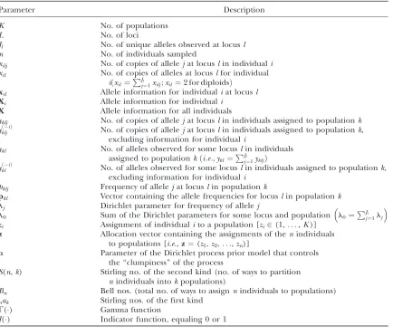
The description of the method entails considerable notation, and in Table 1 we provide a complete list of all the variables we consider.
Data:We assume that we have sampled the alleles forn in-dividuals atLloci. At locusl, we observeJlunique alleles. The number of copies of allelejat locuslin individualiis denoted xilj. Similarly, the number of copies of all alleles observed at locuslin individualiis denotedxil ¼
PJl
j¼1xilj. The allelic in-formation for individualiat locuslis contained in the vector,
xi1¼ ð0;0;0;1;0;0;0;1;0;0Þ
xi2¼ ð0;2;0;0;0;0Þ
xi3¼ ð0;0;0;0;0;0;0;0;0;0;1;0;1;0Þ
xi4¼ ð0;0;2Þ
xi5¼ ð1;0;0;0;1;0;0;0Þ;
where there areL¼5 loci with the loci havingJ1¼10,J2¼6, J3¼14,J4¼3,J5¼8 observed alleles. This example individual is homozygous at the second and fourth loci and heterozygous at the others. We denote the complete information for theith individual asXi¼(xi1,xi2,. . .,xiL). Similarly, we denote the information for all of thenindividuals asX¼(X1,X2,. . .,Xn).
The combinatorics of assigning individuals to populations:
Thenindividuals are assigned to one ofKpopulations. The information on the assignment of individuals to populations is contained in an assignment vector,z. Specifically, the assign-ment of individualito populationkis denotedzi¼k, where zi2(1,. . .,K). An example of an assignment vector forn¼5 individuals might look like
z¼ ð2;1;1;1;3Þ:
Here there are K ¼ 3 populations with individuals 2, 3, and 4 being assigned to the same population. The number of individuals that are assigned to the ith population is denotedhi.
The number of ways to assign n individuals to one ofk populations is given by the Stirling numbers of the second kind,
Sðn;kÞ ¼1 k!
Xk1
i¼0
ð1Þik
i
ðkiÞn:
For our example ofn¼5 individuals andK¼3 populations, there are a total ofS(5, 3)¼25 ways to partition the individuals among populations. The total number of ways to partition n individuals among populations is given by the Bell num-bers (Bell1934). The Bell numbers,B
n, are calculated as the sum
Bn¼
Xn
i¼0 Sðn;iÞ:
For example,n¼5 individuals can be partitioned among 1, 2, 3, 4, or 5 populations. The total number of ways to assign individuals to populations, then, is
P5
i¼0Sð5;iÞ ¼01111512511011¼52:
We label possible partitions of the individuals into pop-ulations using the restricted growth function notation of
TABLE 1
Definitions of parameters used in this study
Parameter Description
K No. of populations
L No. of loci
Jl No. of unique alleles observed at locusl
n No. of individuals sampled
xilj No. of copies of allelejat locuslin individuali xil No. of copies of alleles at locuslfor individual
iðxil ¼PJlj¼1xilj;xil ¼2 for diploidsÞ
xil Allele information for individualiat locusl
Xi Allele information for individuali
X Allele information for all individuals
yklj No. of copies of allelejat locuslin individuals assigned to populationk yðkljiÞ No. of copies of allelejat locuslin individuals assigned to populationk,
excluding information for individuali
ykl No. of alleles observed for some locuslin individuals assigned to populationkði:e:;ykl¼
PJl j¼1ykljÞ
yðkliÞ No. of alleles observed for some locuslin individuals assigned to populationk, excluding information for individuali
pklj Frequency of allelejat locuslin populationk
pkl Vector containing the allele frequencies for locuslin populationk
lj Dirichlet parameter for frequency of allelej
l0 Sum of the Dirichlet parameters for some locus and population l0¼ PJl
j¼1lj
zi Assignment of individualito a population [zi2(1,. . .,K)]
z Allocation vector containing the assignments of thenindividuals to populations [i.e.,z¼(z1,z2,. . .,zn)]
a Parameter of the Dirichlet process prior model that controls the ‘‘clumpiness’’ of the process
S(n,k) Stirling no. of the second kind (no. of ways to partition nindividuals intokpopulations)
Bn Bell nos. (total no. of ways to assignnindividuals to populations) nak Stirling nos. of the first kind
G() Gamma function
Stantonand White(1986), where elements are sequentially
numbered with the constraint that the index numbers for two individuals are the same if they are found in the same population. For example, the allocation vectorz¼ (2, 1, 1, 1, 3) is described using the restricted growth function notation as 1, 2, 2, 2, 3.
Assigning individuals to populations when K is fixed:
Pritchardet al. (2000) examined the case where the number
of populations,K, is considered to be fixed, but the allocation vector,z, is treated as a random variable. They treated the problem in a Bayesian context. In a Bayesian framework, infer-ences are based upon the posterior probability of a parameter. For the problem of assigning individuals to populations, ideally one would calculate the posterior probability of an assignment vectorf(zjX,K), which can be calculated using Bayes’ theorem as
fðzjX;KÞ ¼fðXjz;KÞfðzjKÞ fðXjKÞ :
Probabilities of assignment vectors, however, are rarely cal-culated. The posterior probability of an assignment vector cannot be calculated analytically and must instead be approx-imated using a numerical technique such as MCMC. When the number of individuals is large, there are a vast number of possible assignment vectors and the posterior probability for even the most probable can be quite small and difficult to approximate accurately. For example, whenn¼200 andK¼5 there are a total ofS(200, 5)¼5.186310137possible ways to partition individuals among populations; in this case, even the best partitioning scheme might have a tiny probability that is difficult or impossible to approximate using a method like MCMC.
Instead of calculating the probability of an assignment vector, the more practical solution is to calculate the marginal posterior probability of assigning individualito populationk,
fðzi¼kjX;KÞ ¼
fðXjzi¼k;KÞfðzi¼kjKÞ
fðXjKÞ ;
wheref(Xjzi¼k,K) is the likelihood (the probability of the observations when individualiis assigned to populationk) and f(zi¼kjK) is the prior probability of assigning individualito populationk. This is the approach taken by Pritchardet al.
(2000). They assume a uniform prior on populations, so that f(zi¼kjK)¼1/K. For their model without admixture and assuming that the allele frequencies for each population are in linkage equilibrium and in Hardy–Weinberg equilibrium, the probability of the information for individualiis
fðXijzi¼k;K;pk1;. . .;pkLÞ ¼
YL
l¼1
YJl
j¼1 pxilj
klj
!
:
Herepkljis the frequency of allelejat locuslin populationk; the vectorpkl contains the allele frequencies for locus l in populationk. The probability of the observations on all of the individuals is the product of the likelihoods for the individuals.
Pritchardet al. (2000), following the lead of Baldingand
Nichols(1995) and Rannalaand Mountain(1997), assume
that the allele frequencies have a flat Dirichlet prior probabil-ity distribution. The Dirichlet distribution has probabilprobabil-ity density
fðpklÞ ¼QJGðl0Þ l
j¼1GðljÞ
YJl
j¼1 plj1
klj ;
where l0¼ PJl
j¼1lj and G() is the Gamma function. The flat Dirichlet distribution has alllj¼1.
Pritchard et al. (2000) do not condition upon any
particular combination of allele frequencies when calculating the likelihood, instead integrating the likelihood over all possible combinations of allele frequencies, each combination being weighted by its probability under a flat Dirichlet prior. They then approximate the posterior probability using MCMC. Specifically, the program Structure—a program that imple-ments the method outlined above—uses Gibbs sampling to first sample allele frequencies for each locus conditioned on the assignment of individuals to populations. They then use another Gibbs sampling step to assign individuals to popula-tions (assuming that the allele frequencies are fixed). Repe-tition of these two Gibbs sampling steps allows the program Structure to integrate over allele frequencies and assignment vectors. If one is interested in the marginal posterior proba-bility that individualiis assigned to populationk, one simply records the fraction of the time that the individual was as-signed to that population; the fraction of the time the Markov chain has individualiin populationkis a valid approximation of the probability that the individual is assigned to the pop-ulation (Tierney1996).
For the simple problem of assigning individuals to popula-tions without admixture, one does not need to use this two-step Gibbs procedure; one can perform Gibbs sampling on the assignment of individuals to populations while analytically integrating over the possible allele frequencies (a point also made by Pellaand Masuda2006). The Gibbs sampling
pro-cedure works like this: Pick an individual denotedi. Reassign this individual to populationkwith probability
fðzi¼kjXiÞ ¼
fðXijzi¼kÞ1=K
PK
j¼1fðXijzi¼jÞ1=K
:
The likelihood,f(Xijzi¼k), is calculated by integrating over all possible combinations of allele frequencies:
fðXijzi¼kÞ ¼
YL
l¼1
ð
pkl
fðXijzi¼k;pklÞfðpkljXiÞdpkl:
When individual i is placed into population k, the allele frequencies may not follow the prior probability distribution (e.g., a flat Dirichlet distribution) because other individuals may also be included in that population, thus modifying the probability density of different allele frequency combinations. Instead, the allele frequencies are drawn from the posterior probability distribution of allele frequencies for that popula-tion with individualiexcluded. The notationXiis read ‘‘all of the observations, excluding the observations made on in-dividuali.’’ The likelihood is then
fðXijzi¼kÞ
¼Y L l¼1 ð pkl YJl j¼1 pkljxilj
!
Gðll01yklðiÞÞ
QJl
j¼1Gðljl1y
ðiÞ
klj Þ
YJl
j¼1 py
ðiÞ klj1llj1 klj
!
dpkl ð1Þ
¼Y
L
l¼1
Gðll01y ðiÞ
kl Þ
QJl
j¼1Gðljl1y ðiÞ
klj Þ
ð
pkl
YJl
j¼1 pxilj1y
ðiÞ klj 1llj1
klj dpkl
!
: ð2Þ
Here, ykljis the number of copies of allele jat locus l
yklj¼
Xn
i¼1
¼IðziÞxilj;
where I(zi) is an indicator function that equals one if indi-vidual i is assigned to population k (i.e., zi ¼ k) and zero otherwise. The summation ofyklj over all alleles is denoted ykl¼
PJl
j¼1yklj. Finally, the superscript ‘‘(i)’’ indicates that the count excludes individuali.
The integral in Equation 2 can be solved analytically. Re-membering that
ð
p Gða0Þ
QJl
j¼1GðajÞ
YJl
j¼1 paj1
j dp¼1
we have
Gðxil1y
ðiÞ
kl 1ll0Þ
QJl
j¼1Gðxilj1ykljðiÞ1lljÞ
3 ð
pkl YJl
j¼1 pxilj1y
ðiÞ
klj 1llj1
klj dpkl¼1
ð
pkl YJl
j¼1 pxilj1y
ðiÞ
klj 1llj1
klj dpkl¼
QJl
j¼1Gðxilj1y
ðiÞ
klj 1lljÞ
Gðxil1yðkliÞ1ll0Þ
:
This means that
fðXijzi¼kÞ
¼Y
L
l¼1
GðyklðiÞ1ll0Þ
QJl
j¼1Gðy
ðiÞ
klj 1lljÞ
3 QJl
j¼1Gðxilj1y
ðiÞ
klj 1lljÞ
Gðxil1y
ðiÞ
kl 1ll0Þ
! ð3Þ
¼Y
L
l¼1
GðyklðiÞ1ll0Þ
Gðxil1y
ðiÞ
kl 1ll0Þ
YJl
j¼1
Gðxilj1y
ðiÞ
klj 1lljÞ
GðyðkljiÞ1lljÞ
!
: ð4Þ
This result was first derived by Rannala and Mountain
(1997) and can be used to perform Gibbs sampling only with respect to the assignment of individuals to populations.
Assigning individuals to populations when Kis a random variable:Our goal is to assign individuals to populations while allowing both the allocation vector (z) and the number of populations (K) to both be random variables. To do this we assume that the joint prior probability of the allocation vector and the number of populations follows a Dirichlet process prior (Ferguson1973; Antoniak1974; Pellaand Masuda
2006). Specifically, under the Dirichlet process prior the joint probability ofzandKis
fðz;Kja;nÞ ¼ak
QK
i¼1ðhi1Þ!
Qn
i¼1ða1i1Þ
: ð5Þ
The parameter a is a concentration parameter that deter-mines the degree to which individuals are grouped together into the same population. In fact, the prior probability that two randomly chosen individuals (iandj) are grouped together in the same population is
fðzi¼zjjaÞ ¼
1 11a:
Clearly, whenais small, the prior probability of two individuals finding themselves in the same population is high. Moreover,
the probability of having K populations is obtained by summing over all possible partitions forKpopulations,
fðKja;nÞ ¼ naKa
K
Qn
i¼1ða1i1Þ
;
wherenakis the absolute value of the Stirling numbers of the first kind. Finally, the expected number of populations is
EðKja;nÞ ¼X
n
i¼1
ifðK¼ija;nÞ aln 11n a
:
The Dirichlet process prior model, then, can be understood by considering the following procedure: First, randomly draw the number of populations (K) and the allocation vector (z) from the probability distribution described by Equation 5; then, for each population randomly draw the allele frequen-cies from the Dirichlet probability distribution prior (in this study, we use a flat Dirichlet). We use the word ‘‘Dirichlet’’ in two different senses: first, to describe the prior probability distribution on allele frequencies (this is the ‘‘Dirichlet ability distribution’’) and, second, to describe the prior prob-ability distribution on the allocation vector and on the number of populations (this is the ‘‘Dirichlet process prior’’). Keep in mind that the Dirichlet probability distribution and the Dirichlet process prior are two different probability distributions.
We use Algorithm 3 from Neal (2000) to perform the
numerical integration over the possible allocation vectors and number of populations. Neal(2000) describes a Gibbs
sam-pling scheme for MCMC that works as follows. First, pick an individual,i, and remove it from the allocation vectorz. If the individual was alone in a population, then the population is removed from computer memory, and the total number of populations is decreased by one. Otherwise, the count of the number of individuals in the population,h, is decreased by one. Place individualiinto populationkwith probability
fðzi¼kjzi;XiÞ
¼bhkY
L
l¼1
ð
pkl
fðXijzi¼k;pklÞfðpkljXiÞdpkl
(see Equation 4) and into a new populationk(all by itself) with probability
baY
L
l¼1
ð
pkl
fðXijzi¼k;pklÞfðpklÞdpkl;
wheref(pkl) is the Dirichlet prior density distribution on allele frequencies andbis a normalizing constant.
Computer program:The methods described in this article have been implemented in a computer program called Structurama. The program, written in C11, implements a Gibbs MCMC sampling strategy for assigning individuals to populations when K is fixed and the strategy described by Neal(2000) when the number of populations is treated as a
random variable with a Dirichlet process prior. The program is available for free download from http://www.structurama.org. Each MCMC cycle of the program involves a Gibbs scan of all of the individuals; hence, the total number of MCMC cycles for the analyses of this study is the product of the reported number of MCMC cycles and the number of individuals in the analysis.
MCMC we implement needs only to integrate over the placement of individuals into populations; unlike other implementations, we analytically integrate over allele frequen-cies. Moreover, we implemented (though did not use in this article) a variant of MCMC called Metropolis-coupled Markov chain Monte Carlo [MCMCMC or (MC)3(Geyer1991)]. This
variant of MCMC better allows a Markov chain to explore the parameter space. We recommend not only that MCMCMC be used on difficult problems (those involving, say,$1000 individ-uals), but also that the results be checked carefully by comparing the inferences from multiple chains on the same data.
Summarizing the results of a MCMC analysis of population structure:Considerable attention has been paid to the prob-lem of how to summarize the results of a Bayesian analysis of population structure. The output of a Markov chain can be used to calculate the probabilities of assigning individuals to populations. For example, consider the following (arbitrarily constructed) output from a MCMC analysis of population structure:
Here N is the sample number and K is the number of populations. There are a number of ways to describe the current state of the Markov chain. One way is to simply assign each population an index. The column labeled ‘‘Arbitrary indexing’’ shows this strategy. In fact, this is the strategy taken in the program Structure. The last column shows the labeling of the population partition using the restricted growth function (RGF) notation of Stanton and White (1986).
The main problem with the arbitrary indexing scheme is that the labels are just that, arbitrary. In fact, if the Markov chain mixes properly, then it should be able to explore other, equivalent, indexing schemes for the partition. For example, the first and fifth samples shown in the example MCMC output, above, are equivalent in that they specify the same partition of individuals to populations. (Note that the first and fifth samples have the same description using the restricted growth function notation.) When there areK populations, there areK! equivalent arbitrary indexing schemes that can be applied to describe the same partition of individuals among populations. In other words, if the Markov chain mixes well (i.e., properly explores the parameter space), then the following six indexing schemes for the same partition should be visited by the Markov chain equally often: (1 1 1 2 2 2 3 3 3), (1 1 1 3 3 3 2 2 2), (2 2 2 1 1 1 3 3 3), (2 2 2 3 3 3 1 1 1), (3 3 3 1 1 1 2 2 2), (3 3 3 2 2 2 1 1 1). This problem was noted by Pritchard
et al. (2000) and Stephens (2000), but their method for
summarizing the results of the output of a MCMC analysis relies on the fact that in practice, only one of the equivalent labeling schemes for a partition is visited.
Here, we explore a number of different ways to summarize the results of a Bayesian MCMC analysis of population struc-ture. The first method we explore simply summarizes the probability that each of theðn2Þpairs of individuals are in the same population. The approximation of the probability that individuali and individual j are in the same population is simply the fraction of the time they were placed into the same population during the MCMC analysis and does not depend upon the labeling scheme for the partitions. The prior
prob-ability of any two individuals falling into the same population under the Dirichlet process prior is 1/(11a). This means that the Bayes factor in favor of individualsiandjbeing in the same population is
BFðzi¼zjÞ ¼
Prðzi¼zjjXÞ=ð1Prðzi¼zjjXÞÞ
ð1=ð11aÞÞ=ða=ð11aÞÞ
¼Prðzi¼zjjXÞ3a 1Prðzi¼zjjXÞ
:
Lavine and Schervish (1999) argue that Bayes’ factors
should be interpreted as the degree by which an investigator changes his or her mind about a hypothesis after making some observations. In the context of inferring population structure, the Bayes factor would indicate how strongly two individuals are grouped into the same population.
Another strategy we explore for summarizing the results of a Bayesian analysis of population structure relies on a distance on partitions, described by Gusfield(2002). The basic idea is
to find a partitioning of the individuals among populations that minimizes the squared distance to the partitions sampled by the MCMC algorithm (Figure 1). Here, we rely on the interpretation of the mean as minimizing the squared distance to a sample. For example, consider the usual interpretation of the mean ofnreal numbers,x1,x2,. . .,xn. Ifd(xi,m)¼(xim), then the value ofm that minimizesPni¼1dðxi;mÞ2 ism¼x. We consider the partition distance,dðzi;zjÞ, and define the mean partition to be the partition, z, that minimizes
PN
i¼1dðzi;zÞ2, where the summation is over all N of the partitions sampled by the MCMC algorithm. The partition distance,dðzi;zjÞ, is the minimum number of individuals that must be deleted from bothziandzjto make the two induced partitions the same. Equivalently, the partition distance of Gusfield(2002) can be thought of as the minimum number
of elements that must be moved between populations in one of the partitions to make it identical to the other partition. We search for the mean partition using the following algorithm. First, we start with an arbitrarily chosen partition. Here, we start with one of the partitions sampled by the Markov chain. We then attempt to place each element (individual) of the mean partition into each of the other clusters (populations) and also into a cluster all by itself. At each step, we keep track of the mean squared distance to all of the sampled partitions and move to partitions that result in a smaller mean squared distance. The algorithm stops when a partition is found in which perturbation does not result in a smaller mean squared distance to sampled partitions. Our experience is that this algorithm works well in finding the mean partition, even when the starting partition is distant from the sampled partitions.
Figure1.—Example of the calculation of the mean
parti-tion. The mean partition,z, minimizes the sum of the squared distances to the partitions sampled by the MCMC algorithm.
N K Arbitrary indexing RGF indexing
Analysis of real data:We explored the method of Pellaand
Masuda(2006) on three empirical data sets:
1. The first data set we explored is ofn¼216 Impala (Aepyceros melampus) individuals sampled atL¼8 microsatellite loci (Lorenzenet al.2004, 2006).
2. We also examined a data set of n ¼ 155 Taita thrush (Galbuseraet al.2000). Each bird was sampled atL¼7
microsatellite loci. The thrush data were also analyzed by Pritchardet al.(2000).
3. Finally, we examined Orthet al.’s (1998) data onn¼74
Mus musculus individuals sampled from Lake Casitas, California. The Mus data haveL¼7 loci.
We performed 11 analyses for each of the three data sets (Impala, thrush, and Mus). Specifically, we ran analyses in which the number of populations was fixed (K¼1,. . ., 7) and in which the number of populations follows a Dirichlet process prior with a prior mean ofE(K)¼2,E(K)¼5,E(K)¼10, andE(K)¼20. All MCMC analyses were run for a total of 1 million cycles.
Computer simulations: We used computer simulation to explore the statistical behavior of population assignment under the Dirichlet process prior. Specifically, we explored two different models for generating genetic data. First, we simulated data under the Dirichlet process prior. We simu-lated up to 1000 data sets, each consisting ofn¼ 100 indi-viduals under the Dirichlet process withE(K)¼5. This means that each simulated data set might differ in the number of populations (and almost certainly differed in the allocation vector), but that the average number of populations over the replicates was close to five. We explored two scenarios here. First, we varied the number of loci. This allows us to investigate the effect of the number of observations on the performance of the method. We also explored the robustness of the method to misspecification of the ‘‘clumpiness’’ parameter (a) of the Dirichlet process prior. We did this by generating data with a prior mean ofE(K)¼5, but analyzing the data with the prior mean set toE(K)¼5,E(K)¼10, orE(K)¼20. We designed the simulations to also allow us to check the validity of our implementation of the Dirichlet process prior. For example, when data are generated under the Dirichlet process prior and analyzed under the same model conditions [e.g., when we simulated and analyzed data with the prior mean of the number of populations set toE(K)¼5], a 95% credible set of the number of populations should contain the true number of populations with probability 0.95.
We also simulated data under a neutral coalescent model using the programms(Hudson2002). The model assumes an
infinite-sites mutation model and no recombination so that each new mutation results in an unique allele (haplotype). To evaluate the type I error of the Dirichlet process prior method we simulated a single panmictic population withu¼4Neu¼ (0.5, 1, 2, 4), whereNeis the effective population size anduis the mutation rate per generation. Our analyses of these sim-ulations with Structurama suggest that the Dirichlet process prior method has low type I error (i.e.,#5%) in the absence of population structure (see Table 3). While a full exploration of possible demographic models is beyond the scope of this study, a wide range of demographic models is straight-forward to implement using the program ms (see the program documentation, http://home.uchicago.edu/rhudson1/source/ mksamples.html). As a first-pass evaluation of Structurama’s ability to detect population structure, we modeled a symmetric equilibrium island model with 2, 4, and 10 demes of equal size whereu¼4Neu¼(0.5, 1.0, 2.0, 4.0),M¼4Nem¼(0.5, 1.0, 2.0, 4.0), andmis the migration rate per generation. In each case, 100 diploid individuals were sampled in total, with equal numbers of individuals being sampled from each deme. Clearly, this demographic model and sampling scheme are highly simplistic and are intended only to be illustrative. The ms command lines we implemented are listed in theappendix.
A perl script that digests the ms output into Structurama in-put is available on request to P. Andolfatto.
For each simulated data set, we ran a single Markov chain for a total of 100,000 cycles. We thinned the Markov chains by sampling every 25th sample and discarded samples taken during the first 12,500 cycles as the burn-in of the chain. The program Structurama, which can work in a batch-processing mode, was used for analysis of all simulated data.
RESULTS AND DISCUSSION
Figures 2–4 show the results of the analyses of the real data. Each figure shows the mean partition summariz-ing the MCMC samples for a particular analysis. Indi-viduals are arrayed along columns, and each row represents a different analysis. Individuals sharing a color are grouped together into the same population. As expected, the partitions differ when the fixed number
Figure2.—The mean partitions for analyses of the ImapalaAegyceros melampusdata (Lorenzenet al. 2004, 2006). Analyses were
of populations varies. Interestingly, the mean partition is rather insensitive to the choice of the clumpiness parameter,a, when a Dirichlet process prior probability distribution is applied to the assignment vector and the number of populations; note that the same mean partition results when the prior mean of the number of populations is varied fromE(K)¼5 toE(K)¼20.
The problem of summarizing the results of an MCMC analysis of population structure is a difficult one, be-cause the object of estimation—a partition representing the population structure—is not a standard statistical parameter. There is no natural way to order partitions, for example. In many ways, the problem of summarizing a collection of partitions (sampled, from say, a Markov chain) has parallels in the phylogenetics literature, where the object of inference is a phylogenetic tree. Trees, like partitions, cannot be naturally ordered. In the phylogenetics literature, a number of solutions have been considered, including consensus trees. Several methods have been suggested for summarizing the results of a MCMC analysis of population structure. As mentioned earlier, one solution is to arbitrarily assign indexes to populations. Although other choices of indexes will result in the same partition of individuals to populations, in practice the MCMC may fail to visit
these alternative labeling schemes; the summary of the population index to which each individual is assigned, then, may be useful. Dawsonand Belkhir(2001)
sug-gest a clustering method for summarizing the results of an MCMC analysis of population structure. Their method applies a hierarchical clustering algorithm to identify well-supported clusters of individuals. Stephens(2000),
on the other hand, takes a decision theoretic approach and attempts to find a partition that minimizes the posterior expected loss. Our method of constructing a mean partition best fits the decision theoretic ap-proach, with a loss function that is the squared distance between a sampled partition and the true partition. The weakness of our approach is that it relies upon a distance on partitions (one described by Gusfield2002), which
is itself arbitrary. Unfortunately, only the Gusfield
(2002) metric on partitions exists; other metrics on par-titions are surely possible and could be usefully applied to the problem of summarizing the results of a MCMC analysis of population structure.
Figure 5 shows an alternative method for summariz-ing the results of the MCMC analysis of population structure. These plots—dubbed ‘‘plaid plots’’ by one of us—show the probabilities of all possible pairs of indi-viduals being grouped together into the same population.
Figure3.—The mean partitions for analyses of the Taita thrush data (Galbuseraet al.2000). Analyses were performed in which
the number of populations was fixed (K¼1,K¼2,K¼3,K¼4,K¼5,K¼6,K¼7) or in which the number of populations was a random variable with a Dirichlet process prior [E(K)¼2,E(K)¼5,E(K)¼10,E(K)¼20]. The assignment of individuals (boxes) is indicated by color.
Figure4.—The mean partitions for analyses of theMus musculusdata (Orthet al.1998). Analyses were performed in which the
The plots are rather complicated to read, at least on a first pass. The top left corner of each triangle shows the probability of individuals 1 and 2 being grouped into the same population. The top right corner of each graph shows the probability of individuals 1 and n
finding themselves in the same population. Finally, the bottom right corner of each plot shows the probability of individualsnandn1 being grouped together in the same population. The color red indicates a probability
.0.9 of two individuals being in the same population. One finds blocks of individuals all of whom share a high probability of being grouped together in the same population, but a low probability of being grouped with any other individuals (this is indicated by the ‘‘stair case’’-like pattern of red coloration in the plots). Figure 5 also shows the Bayes factors for all pairs of individuals being grouped together in the same population. The Bayes factor measures the strength of the evidence grouping individuals together. Formally, it measures the
degree by which an individual changes his or her mind about the grouping of a pair of individuals after ob-serving the genetic data. Generally speaking, Bayes’ factors .10 are considered ‘‘positive’’ or ‘‘strong’’ evi-dence in favor of a hypothesis ( Jeffreys1961), in this
case the hypothesis being that individuals i and jare in the same population. Similarly, a Bayes factor,1
10 can be considered strong evidence against two individ-uals being in the same population. One advantage of the plaid plots is that they are invariant to the labeling of populations; all that is considered is whether two individuals are assigned to the same population or to different populations.
How many populations are required to explain the data? Figure 6 shows the approximate marginal like-lihoods for varying numbers of populations for the three empirical data sets. The marginal likelihoods were calculated by taking the harmonic mean of the like-lihoods for samples taken by the MCMC algorithm
Figure 5.—The probabilities and Bayes’
fac-tors of all pairs of individuals being grouped to-gether into the same population. Each triangle shows all ðn2Þ pairs of individuals. The top left corner of a triangle shows the probability/Bayes’ factor for individuals 1 and 2, the top right corner of the triangle shows the probability/Bayes’ fac-tor for individuals 1 andn, and the bottom cor-ner of the triangle shows the probability/Bayes’ factor for individuals n 1 and n. Generally speaking, Bayes’ factors.10 are strong evidence for two individuals being grouped together in the same population whereas Bayes’ factors ,1
(Newton and Raftery 1994) when the number of
populations is considered fixed. Note that it is difficult to explain the data with only a few populations (e.g., one or two), but that the marginal likelihoods are similar for larger numbers of populations. Typically, one picks the number of populations that is a compromise between the ability to explain the data (i.e., pickingKsuch that the marginal likelihood is high) and parsimony (i.e., pickingKas small as possible). One can do this using, for example, the Akaike information criterion (Akaike
1973) in which the marginal likelihood is penalized by the number of parameters (populations). Our approach involves sampling only assignments of individuals to
populations and analytically integrates over uncertainty in allele frequencies; it is likely that our estimates of the marginal likelihood are more accurate than approaches that use MCMC to integrate over uncertainty in allele frequencies. Even so, Raftery et al.(2006) point out
that while the harmonic mean is an unbiased estimator, it can have an infinite variance and is generally an unstable estimate of the marginal likelihood.
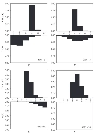
Inference of the number of populations is automatic to the procedure when the number of populations and the assignment of individuals to populations are both considered random variables that follow a Dirichlet process prior. Figure 7 shows the prior and posterior probability distributions forKfor four analyses of the Impala data set. The maximum posterior probability (MAP) estimate of the number of populations isK¼4 for three of the four analyses. When the prior mean of the number of populations isE(K)¼2,E(K)¼5, or
E(K)¼10, most of the posterior probability is onK¼4. Only when the prior mean isE(K)¼20 does the MAP estimate of the number of populations shift toK¼5. In this study, we assumed a fixed value for the concentra-tion parameter,a. For ease of interpretation, we seta
using the prior mean on the number of populations; that is, we first chose a prior mean forKand then found the a that gives the desired prior mean. In some Bayesian analyses under a Dirichlet prior process, however, a probability distribution is put on the con-centration parameter,a. Typically, a Gamma hyperprior is placed ona. We implemented the Gamma hyperprior in Structurama, but did not explore the effect of this approach on the inferences.
How well can we expect to assign individuals to populations under the Dirichlet process model? We used simulation to explore the statistical behavior of the method. Table 2 summarizes the results for our first set of simulations. The first set of simulations was designed to explore the behavior of the method in a best-case scenario, in which all of the assumptions of the method are satisfied. We simulated data under a Dirichlet process prior in which E(K) ¼ 5. We then analyzed the data under precisely the same model [i.e., with
E(K)¼5] and under situations in which the prior is misspecified [i.e., withE(K)¼10 andE(K)¼20]. In the simulations, we varied the number of loci fromL¼
10 to L ¼100. Note that the average distance of the partitions sampled by the MCMC algorithm to the true partition (zT) decreases as the number of loci increases.
This result is to be expected; as the number of obser-vations increases, inferences about the population assignment become more accurate. Here, we use the partition distance to measure the distance of the sampled partitions to the true partition in each simula-tion (Gusfield2002). Also, as expected, inferences are
less accurate when the concentration parameter,a, is misspecified. However, the effect of number of loci is much stronger than the effect of prior misspecification.
Figure6.—The marginal likelihoods Pr(XjK) when the
number of populations (K) is fixed to different values (K ¼ 1, 2, . . ., 7). (a) Impala data (Lorenzen et al. 2004,
2006); (b) Taita thrush data (Galbusera et al. 2000); (c)
We also noted the coverage probability for all the simulations. For each MCMC analysis of the simulated data, we constructed a 95% credible set for the number of populations. If the method is behaving correctly, a 95% credible set should contain the true number of populations 95% of the time. One can see that when the
prior forais not misspecified, the coverage (probability that the 95% credible set contains the true number of populations) is0.95. However, when the prior model is misspecified, the 95% credible set contains the true number of populations with a probability ,0.95. For example, in one of the simulations ofL¼10 loci, data
Figure 7.—The prior, Pr(K), and posterior,
Pr(KjX), probability distributions for the num-ber of populations for the Impala data set when the prior mean of the number of populations varies.
TABLE 2
Results of simulations under the Dirichlet process prior withE(K)¼5
n L E(K) E[E(KjX)KT] Coverage E[d(z,zT)] No. replicates
100 10 5 0.056 0.954 5.08 1000
10 1.034 0.896 5.63
20 2.656 0.527 6.77
100 20 5 0.014 0.954 1.20 1000
10 0.400 0.940 1.36
20 0.955 0.817 1.70
100 100 5 0.002 0.950 0.016 500
were simulated with a prior mean of 5, but analyzed assuming a prior mean for the number of populations of 20. In this set of simulations, the 95% credible set contained the true number of populations only 53%
of the time. Importantly, the simulations suggest that misspecification of the prior on the number of popula-tions becomes less important when the data have many loci. For instance, the coverage probability for the TABLE 3
Results of simulations under a population genetics model when there is one population and the prior mean of the number of populations is 5, 10, or 20
E[E(KjX)KT] E[d(z, zT)] Coverage
KT L u 5 10 20 5 10 20 5 10 20
1 10 0.5 0.04 0.08 0.15 0.04 0.08 0.16 0.98 0.97 0.97
1 10 1.0 0.01 0.03 0.06 0.01 0.03 0.06 0.97 0.95 0.96
1 10 2.0 0.02 0.04 0.07 0.02 0.04 0.08 0.98 0.99 0.95
1 10 4.0 0.04 0.07 0.14 0.05 0.08 0.14 0.97 0.91 0.95
1 100 0.5 0.00 0.00 0.00 0.00 0.00 0.00 0.98 0.97 0.96
1 100 1.0 0.00 0.00 0.00 0.00 0.00 0.00 0.93 0.93 0.95
1 100 2.0 0.00 0.00 0.00 0.00 0.00 0.00 0.98 0.95 0.94
1 100 4.0 0.00 0.00 0.00 0.00 0.00 0.00 0.97 0.87 0.99
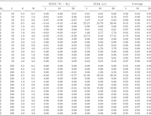
TABLE 4
Results of simulations under a population genetics model when there are two populations and the prior mean of the number of populations is 5, 10, or 20
E[E(KjX)KT] E[d(z, zT)] Coverage
KT L u M 5 10 20 5 10 20 5 10 20
2 10 0.5 0.5 0.00 0.00 0.01 0.01 0.01 0.02 0.92 0.94 0.95
2 10 0.5 1.0 0.01 0.01 0.00 0.63 0.63 0.16 0.97 0.90 0.94
2 10 0.5 2.0 0.07 0.09 0.07 5.27 6.18 6.64 0.89 0.90 0.93
2 10 0.5 4.0 0.44 0.43 0.46 25.21 24.79 26.84 0.53 0.56 0.57
2 10 1.0 0.5 0.00 0.00 0.00 0.00 0.00 0.00 0.95 0.93 0.96
2 10 1.0 1.0 0.00 0.00 0.00 0.01 0.01 0.01 0.97 0.96 0.95
2 10 1.0 2.0 0.03 0.03 0.01 1.68 2.17 1.70 0.93 0.91 0.97
2 10 1.0 4.0 0.22 0.35 0.28 12.74 0.43 17.15 0.73 0.66 0.72
2 10 2.0 0.5 0.00 0.00 0.00 0.00 0.00 0.00 0.92 0.98 0.98
2 10 2.0 1.0 0.00 0.00 0.00 0.00 0.00 0.00 0.96 0.96 0.97
2 10 2.0 2.0 0.01 0.02 0.03 0.02 0.03 0.04 0.96 0.99 0.94
2 10 2.0 4.0 0.10 0.08 0.05 5.73 4.76 3.78 0.84 0.89 0.91
2 10 4.0 0.5 0.00 0.00 0.00 0.00 0.00 0.00 0.96 0.93 0.90
2 10 4.0 1.0 0.00 0.00 0.00 0.00 0.00 0.00 0.93 0.94 0.94
2 10 4.0 2.0 0.00 0.00 0.01 0.01 0.01 0.01 0.95 0.97 0.95
2 10 4.0 4.0 0.00 0.01 0.02 0.04 0.05 0.56 0.97 0.96 0.96
2 100 0.5 0.5 0.00 0.00 0.00 0.00 0.00 0.00 0.91 0.96 0.96
2 100 0.5 1.0 0.00 0.00 0.00 0.00 0.00 0.00 0.88 0.92 0.97
2 100 0.5 2.0 0.00 0.02 0.01 0.00 1.00 0.50 0.95 0.92 0.92
2 100 0.5 4.0 0.82 0.79 0.77 41.00 39.50 38.50 0.18 0.19 0.23
2 100 1.0 0.5 0.00 0.00 0.00 0.00 0.00 0.00 0.97 0.98 0.91
2 100 1.0 1.0 0.00 0.00 0.00 0.00 0.00 0.00 0.95 0.95 0.97
2 100 1.0 2.0 0.00 0.00 0.00 0.00 0.00 0.00 0.93 0.95 0.95
2 100 1.0 4.0 0.25 0.30 0.24 12.50 15.00 12.00 0.73 0.69 0.73
2 100 2.0 0.5 0.00 0.00 0.00 0.00 0.00 0.00 0.94 0.93 0.97
2 100 2.0 1.0 0.00 0.00 0.00 0.00 0.00 0.00 0.94 0.91 0.94
2 100 2.0 2.0 0.00 0.00 0.00 0.00 0.00 0.00 0.99 0.93 0.98
2 100 2.0 4.0 0.00 0.00 0.00 0.00 0.00 0.00 0.95 0.93 0.96
2 100 4.0 0.5 0.00 0.00 0.00 0.00 0.00 0.00 0.92 0.96 0.93
2 100 4.0 1.0 0.00 0.00 0.00 0.00 0.00 0.00 0.93 0.97 0.94
2 100 4.0 2.0 0.00 0.00 0.00 0.00 0.00 0.00 0.94 0.95 0.95
number of populations did not appear to be affected for the simulations ofL¼100 loci. Finally, the bias in the estimates of the number of populations appears to be moderate in the simulations under the Dirichlet process prior. We measured bias as the difference between the average of the number of populations sampled by the MCMC algorithm and the true number of populations (E[E(KjX)KT]). Generally, the number of
popula-tions was slightly overestimated when the prior mean chosen for the analysis was larger than the prior mean used to simulate the data.
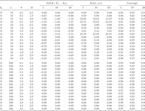
In our second set of simulations, we simulated data under a model completely different from the Dirichlet process prior model under which the data were ana-lyzed. Specifically, we simulated data under a population genetics model with K¼1, K¼ 2,K¼ 4, orK ¼10 populations. We allowed u ¼ 4Nu to vary and also assumed a symmetric migration model between pop-ulations with varying migration rates (M¼4Nm). Tables 3–6 summarize the results of these simulations. Again,
we measured the accuracy of the method as the average distance of the sampled partitions to the true partition. We also noted the bias (the degree by which the number of populations is over- or underestimated) and the coverage probability (the probability that a 95% credi-ble set contains the true number of populations). Because there were only 100 simulations for each combination of parameter values, one should take the values for the coverage probabilities with a grain of salt; it is difficult to accurately determine coverage probabil-ities with only 100 replicates. Generally speaking, the simulations show that inferences of population struc-ture are more accurate when (1) more loci are used, (2) migration rates are low, and (3)uis large.
Generally speaking, the results of the simulation study are in accord with what intuition would suggest: (1) Increasing the number of loci improves the ability of the method to correctly identify the partition, (2) estima-tion can suffer when the parameter of the Dirichlet process model,a, is misspecified, and (3) inference of TABLE 5
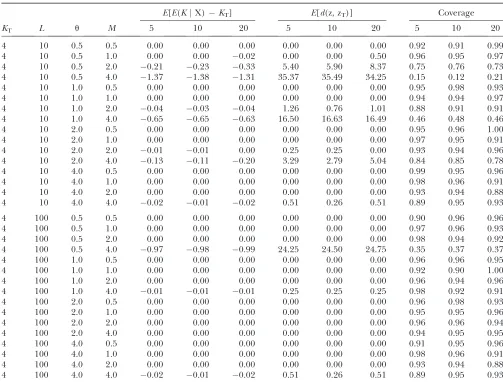
Results of simulations under a population genetics model when there are four populations and the prior mean of the number of populations is 5, 10, or 20
E[E(KjX)KT] E[d(z, zT)] Coverage
KT L u M 5 10 20 5 10 20 5 10 20
4 10 0.5 0.5 0.00 0.00 0.00 0.00 0.00 0.00 0.92 0.91 0.99
4 10 0.5 1.0 0.00 0.00 0.02 0.00 0.00 0.50 0.96 0.95 0.97
4 10 0.5 2.0 0.21 0.23 0.33 5.40 5.90 8.37 0.75 0.76 0.73
4 10 0.5 4.0 1.37 1.38 1.31 35.37 35.49 34.25 0.15 0.12 0.21
4 10 1.0 0.5 0.00 0.00 0.00 0.00 0.00 0.00 0.95 0.98 0.93
4 10 1.0 1.0 0.00 0.00 0.00 0.00 0.00 0.00 0.94 0.94 0.97
4 10 1.0 2.0 0.04 0.03 0.04 1.26 0.76 1.01 0.88 0.91 0.91
4 10 1.0 4.0 0.65 0.65 0.63 16.50 16.63 16.49 0.46 0.48 0.46
4 10 2.0 0.5 0.00 0.00 0.00 0.00 0.00 0.00 0.95 0.96 1.00
4 10 2.0 1.0 0.00 0.00 0.00 0.00 0.00 0.00 0.97 0.95 0.91
4 10 2.0 2.0 0.01 0.01 0.00 0.25 0.25 0.00 0.93 0.94 0.96
4 10 2.0 4.0 0.13 0.11 0.20 3.29 2.79 5.04 0.84 0.85 0.78
4 10 4.0 0.5 0.00 0.00 0.00 0.00 0.00 0.00 0.99 0.95 0.96
4 10 4.0 1.0 0.00 0.00 0.00 0.00 0.00 0.00 0.98 0.96 0.91
4 10 4.0 2.0 0.00 0.00 0.00 0.00 0.00 0.00 0.93 0.94 0.88
4 10 4.0 4.0 0.02 0.01 0.02 0.51 0.26 0.51 0.89 0.95 0.93
4 100 0.5 0.5 0.00 0.00 0.00 0.00 0.00 0.00 0.90 0.96 0.96
4 100 0.5 1.0 0.00 0.00 0.00 0.00 0.00 0.00 0.97 0.96 0.93
4 100 0.5 2.0 0.00 0.00 0.00 0.00 0.00 0.00 0.98 0.94 0.92
4 100 0.5 4.0 0.97 0.98 0.99 24.25 24.50 24.75 0.35 0.37 0.37
4 100 1.0 0.5 0.00 0.00 0.00 0.00 0.00 0.00 0.96 0.96 0.95
4 100 1.0 1.0 0.00 0.00 0.00 0.00 0.00 0.00 0.92 0.90 1.00
4 100 1.0 2.0 0.00 0.00 0.00 0.00 0.00 0.00 0.96 0.94 0.96
4 100 1.0 4.0 0.01 0.01 0.01 0.25 0.25 0.25 0.98 0.92 0.91
4 100 2.0 0.5 0.00 0.00 0.00 0.00 0.00 0.00 0.96 0.98 0.93
4 100 2.0 1.0 0.00 0.00 0.00 0.00 0.00 0.00 0.95 0.95 0.96
4 100 2.0 2.0 0.00 0.00 0.00 0.00 0.00 0.00 0.96 0.96 0.94
4 100 2.0 4.0 0.00 0.00 0.00 0.00 0.00 0.00 0.94 0.95 0.95
4 100 4.0 0.5 0.00 0.00 0.00 0.00 0.00 0.00 0.91 0.95 0.96
4 100 4.0 1.0 0.00 0.00 0.00 0.00 0.00 0.00 0.98 0.96 0.91
4 100 4.0 2.0 0.00 0.00 0.00 0.00 0.00 0.00 0.93 0.94 0.88
population structure is more reliable whenuis large and
M (migration rates) are low. The main result of the simulations, however, is not intuitive: One can accu-rately infer the number of populations in a sample using genetic data under a Dirichlet process model. Impor-tantly, the number of loci necessary to accurately infer the number of populations is moderate in size and in the range of many published studies of population structure. Also, one can accurately infer the number of populations even when the parameter of the Dirichlet process model is misspecified (as long as the number of loci is moderately large).
Demographic models that are relevant to real pop-ulations are likely to be much more complex than the simple symmetric island model we have explored. In addition, markers used to infer population structure are often ascertained in a smaller sample of individuals and geographic sampling schemes can vary widely from study to study. Fortunately, Structurama is easy to use
in conjunction with programs like ms (Hudson 2002;
seematerials and methods) and it is straightforward
to evaluate the program’s performance under virtually any arbitrary sampling scheme and demographic model. Future work could concentrate on the relative performance of different methods for inferring pop-ulation structure. This work might benefit from consid-eration of the methods we devised in this article to measure the accuracy of population structure methods (such as the application of a distance on partitions).
This work was supported by National Science Foundation grant DEB-0445453 and National Institutes of Health grant GM-069801 awarded to J.P.H.
LITERATURE CITED
Akaike, H., 1973 Information theory as an extension of the
maxi-mum likelihood principle, pp. 267–281 in Second International Symposium on Information Theory, edited by B. N. Petrovand F.
Csaki. Akademiai Kiado, Budapest.
TABLE 6
Results of simulations under a population genetics model when there are 10 populations and the prior mean of the number of populations is 5, 10, or 20
E[E(KjX)KT] E[d(z, zT)] Coverage
KT L u M 5 10 20 5 10 20 5 10 20
10 10 0.5 0.5 0.00 0.00 0.00 0.00 0.00 0.00 0.95 0.97 0.91
10 10 0.5 1.0 0.07 0.09 0.06 0.70 0.90 0.60 0.90 0.85 0.90
10 10 0.5 2.0 1.08 1.20 1.18 10.85 12.04 11.87 0.38 0.24 0.27
10 10 0.5 4.0 5.53 5.25 5.37 55.71 53.04 54.33 0.01 0.00 0.00
10 10 1.0 0.5 0.00 0.00 0.00 0.00 0.00 0.00 0.95 0.98 1.00
10 10 1.0 1.0 0.01 0.03 0.02 0.10 0.30 0.20 0.94 0.88 0.95
10 10 1.0 2.0 0.30 0.34 0.32 3.01 3.41 3.21 0.68 0.71 0.68
10 10 1.0 4.0 2.51 2.54 2.51 25.33 25.63 25.41 0.06 0.05 0.07
10 10 2.0 0.5 0.00 0.00 0.00 0.00 0.00 0.00 0.92 0.96 0.95
10 10 2.0 1.0 0.00 0.01 0.00 0.00 0.10 0.00 0.95 0.97 0.95
10 10 2.0 2.0 0.07 0.08 0.05 0.70 0.80 0.50 0.88 0.89 0.90
10 10 2.0 4.0 0.70 0.74 0.59 7.08 7.52 6.09 0.43 0.44 0.55
10 10 4.0 0.5 0.00 0.00 0.00 0.00 0.00 0.00 0.96 0.96 0.97
10 10 4.0 1.0 0.00 0.01 0.01 0.00 0.10 0.10 0.91 0.95 0.92
10 10 4.0 2.0 0.03 0.06 0.09 0.30 0.60 0.90 0.94 0.87 0.90
10 10 4.0 4.0 0.30 0.25 0.35 3.14 2.65 3.80 0.68 0.72 0.66
10 100 0.5 0.5 0.00 0.00 0.00 0.00 0.00 0.00 0.95 0.98 0.95
10 100 0.5 1.0 0.00 0.00 0.00 0.00 0.00 0.00 0.95 0.91 0.94
10 100 0.5 2.0 0.00 0.00 0.00 0.00 0.00 0.00 0.93 0.97 0.94
10 100 0.5 4.0 0.42 0.51 0.43 4.20 5.10 4.30 0.63 0.60 0.65
10 100 1.0 0.5 0.00 0.00 0.00 0.00 0.00 0.00 0.93 0.97 0.96
10 100 1.0 1.0 0.00 0.00 0.00 0.00 0.00 0.00 1.00 0.93 0.93
10 100 1.0 2.0 0.00 0.00 0.00 0.00 0.00 0.00 0.96 0.91 0.94
10 100 1.0 4.0 0.00 0.00 0.00 0.00 0.00 0.00 0.91 0.96 0.93
10 100 2.0 0.5 0.00 0.00 0.00 0.00 0.00 0.00 0.92 0.91 0.95
10 100 2.0 1.0 0.00 0.00 0.00 0.00 0.00 0.00 0.91 0.95 0.96
10 100 2.0 2.0 0.00 0.00 0.00 0.00 0.00 0.00 0.97 0.94 0.96
10 100 2.0 4.0 0.00 0.00 0.00 0.00 0.00 0.00 0.92 0.95 0.92
10 100 4.0 0.5 0.00 0.00 0.00 0.00 0.00 0.00 0.96 0.91 0.97
10 100 4.0 1.0 0.00 0.00 0.00 0.00 0.00 0.00 0.99 0.93 0.99
10 100 4.0 2.0 0.00 0.00 0.00 0.00 0.00 0.00 0.94 0.93 0.95
Andolfatto, P., and M. Przeworski, 2000 A genome-wide
depar-ture from the standard neutral model in natural populations of Drosophila. Genetics156:257–268.
Antoniak, C. E., 1974 Mixtures of Dirichlet processes with
applica-tions to non-parametric problems. Ann. Stat.2:1152–1174. Balding, D. J., and R. A. Nichols, 1995 A method for quantifying
differentiation between populations at multi-allelic loci and its implications for investigating identity and paternity. Genetica
96:3–12.
Bell, E. T., 1934 Exponential numbers. Am. Math. Mon.41:411–
419.
Corander, J., P. Waldmannand M. J. Sillanpa¨ a¨, 2003 Bayesian
analysis of genetic differentiation between populations. Genetics
163:367–374.
Corander, J., P. Waldmann, P. Marttinenand M. J. Sillanpa¨ a¨,
2004 BAPS2: enhanced possibilities for the analysis of popula-tion structure. Bioinformatics20:2363–2369.
Dawson, K. J., and K. Belkhir, 2001 A Bayesian approach to the
identification of panmictic populations and the assignment of in-dividuals. Genet. Res.78:59–77.
Evanno, G., S. Regnautand J. Goudet, 2005 Detecting the
num-ber of clusters of individuals using the software Structure: a sim-ulation study. Mol. Ecol.14:2611–2620.
Falush, D., M. Stephensand J. K. Pritchard, 2003 Inference of
population structure using multilocus genotype data: linked loci and correlated allele frequencies. Genetics164:1567–1587. Ferguson, T. S., 1973 A Bayesian analysis of some nonparametric
problems. Ann. Stat.1:209–230.
Galbusera, P., L. Lens, E. Waiyaki, T. Schenckand E. Mattysen,
2000 Effective population size and gene flow in the globally, critically endangered Taita thrush,Turdus helleri. Conserv. Genet.
1:45–55.
Geyer, C. J., 1991 Markov chain Monte Carlo maximum likelihood,
pp. 156–163 inComputing Science and Statistics: Proceedings of the 23rd Symposium on the Interface, edited by E. M. Keramidas.
Inter-face Foundation, Fairfax Station, VA.
Green, P. J., 1995 Reversible jump MCMC computation and
Bayes-ian model determination. Biometrika82:711–732.
Gusfield, D., 2002 Partition-distance: a problem and class of perfect
graphs arising in clustering. Inform. Process. Lett.82:159–164. Hammer, M. F., F. Blackmer, D. Garrigan, M. W. Nachmanand J. A.
Wilder, 2003 Human population structure and its effects on
sampling Y chromosome sequence variation. Genetics 164:
1495–1509.
Holsinger, K. E., P. O. Lewisand D. K. Dey, 2002 A Bayesian
ap-proach to inferring population structure from dominant markers. Mol. Ecol.11:1157–1164.
Hudson, R. R., 2002 Generating samples under a Wright-Fisher
neutral model of genetic variation. Bioinformatics18:337–338. Jeffreys, H., 1961 Theory of Probability, Ed. 3. Oxford University
Press, Oxford.
Lavine, M., and M. J. Schervish, 1999 Bayes factors: what they are
and what they are not. Am. Stat.53:119–122.
Leo, N. P., J. M. Hughes, X. Yang, S. K. S. Poudel, W. G. Brogdon
et al., 2005 The head and body lice of humans are genetically distinct (Insecta: Phthiraptera, Pediculidae): evidence from dou-ble infestations. Heredity95:34–40.
Lorenzen, E. D., and H. R. Siegismund, 2004 No suggestion of
hy-bridization between the vulnerable black-faced impala (Aepyceros melampus petersi) and the common impala (A. m. melampus) in Etosha NP, Namibia. Mol. Ecol.13:3007–3019.
Lorenzen, E. D., P. Arctanderand H. R. Siegismund, 2006
Re-gional genetic structuring and evolutionary history of the impala Aepyceros melampus. J. Hered.97:119–132.
Male´ cot, G., 1948 Les Mathe´matiques D l’He´re´dite´. Masson et Cie, Paris.
Michel, A. P., M. J. Ingrasci, B. J. Schemerhorn, M. Kern, G. LeGoff
et al., 2005 Rangewide population genetic structure of the African malaria vector Anopheles funestus. Mol. Ecol.14:4235– 4248.
Moodley, Y., and E. H. Harley, 2005 Population structuring in
mountain zebras (Equus zebra): the molecular consequences of divergent demographic histories. Conserv. Genet.6:953–968. Neal, R. M., 2000 Markov chain sampling methods for Dirichlet
process mixture models. J. Comput. Graph. Stat.9:249–265. Nejsum, P., E. D. Parker, J. Frydenberg, A. Roepstorff, J. Boeset al.,
2005 Ascariasis is a zoonosis in Denmark. J. Clin. Microbiol.43:
1142–1148.
Newton, M. A., and A. E. Raftery, 1994 Approximate Bayesian
in-ference with the weighted likelihood bootstrap. J. R. Stat. Soc. B
56:3–48.
Nielsen, R., 2001 Statistical tests of neutrality in the age of
ge-nomics. Heredity86:641–647.
Ochsenreither, S., K. Kuhls, M. Schaar, W. Presber and G.
Schonian, 2006 Multilocus microsatellite typing as a new tool
for discrimination of Leishmania infantum MON-1 strains. J. Clin. Microbiol.44:495–503.
Orth, A., T. Adama, W. Dinand F. Bonhomme, 1998 Hybridation
naturelle entre deux sous espe´ces de souris domestiqueMus mus-culus domesticus etMus musculus castaneuspre´s de Lake Casitas (Californie). Genome41:104–110.
Pella, J., and M. Masuda, 2006 The Gibbs and split-merge sampler
for population mixture analysis from genetic data with incom-plete baselines. Can. J. Fish. Aquat. Sci.63:576–596.
Pritchard, J. K., M. Stephensand P. Donnelly, 2000 Inference of
population structure using multilocus genotype data. Genetics
155:945–959.
Przeworski, M., 2002 The signature of positive selection at
ran-domly chosen loci. Genetics160:1179–1189.
Raftery, A. E., M. A. Newton, J. M. Satagopanand P. N. Krivitsky,
2006 Estimating the Integrated Likelihood via Posterior Simulation Us-ing the Harmonic Mean Identity(Memorial Sloan-Kettering Cancer Center Department of Epidemiology and Biostatistics Working Paper Series, Working Paper 6).
Rannala, B., and J. L. Mountain, 1997 Detecting immigration by
using multilocus genotypes. Proc. Natl. Acad. Sci. USA94:9197– 9201.
Rosenberg, N. A., J. K. Pritchard, J. L. Weber, H. M. Cann, K. K.
Kidd et al., 2002 Genetic structure of human populations.
Science298:2981–2985.
Small, M. P., A. E. Frye, J. F. Von Bargen and S. F. Young,
2006 Genetic structure of chum salmon (Oncorhynchus keta) pop-ulations in the lower Columbia River: Are chum salmon in Cascade tributaries remnant populations? Conserv. Genet.7:65–78. Song, K. J., and R. C. Elston, 2006 A powerful method of
combin-ing measures of association and Hardy-Weinberg disequilibrium for fine-mapping in case-control studies. Stat. Med.25:105–126. Stanton, D., and D. White, 1986 Constructive Combinatorics.
Springer-Verlag, New York.
Stephens, M., 2000 Dealing with label-switching in mixture models.
J. R. Stat. Soc. Ser. B62:795–809.
Tierney, L., 1996 Introduction to general state-space Markov chain
theory, pp. 59–74 inMarkov Chain Monte Carlo in Practice. Chap-man & Hall, London.
Tsai, H. J., J. Y. Kho, N. Shaikh, S. Choudhry, M. Naqviet al.,
2006 Admixture-matched case-control study: a practical ap-proach for genetic association studies in admixed populations. Hum. Genet.118:626–639.
Wright, S., 1940 Breeding structure of populations in relation to
speciation. Am. Nat.74:232–248.
Wright, S., 1943 Isolation by distance. Genetics28:114–138.
Wright, S., 1951 The genetical structure of populatons. Ann.
Eu-gen.15:323–354.
Yu, J. M., G. Pressoir, W. H. Briggs, I. V. Bi, M. Yamasakiet al.,
2006 A unified mixed-model method for association mapping that accounts for multiple levels of relatedness. Nat. Genet.38:
203–208.
APPENDIX: COMMAND LINES USED FOR MS COALESCENT SIMULATIONS TO EVALUATE THE PERFORMANCE OF STRUCTURAMA
One population (panmixia):
./ms 200 10000 -t 0.5.ms.t0.5_p1 ./ms 200 10000 -t 1.ms.t1_p1 ./ms 200 10000 -t 2.ms.t1_p2 ./ms 200 10000 -t 4.ms.t1_p4
Two populations:
./ms 200 10000 -t 0.5 -I 2 100 100 0.5.ms.t0.5_p2_m0.5 ./ms 200 10000 -t 0.5 -I 2 100 100 1.ms.t0.5_p2_m1 ./ms 200 10000 -t 0.5 -I 2 100 100 2.ms.t0.5_p2_m2 ./ms 200 10000 -t 0.5 -I 2 100 100 4.ms.t0.5_p2_m4 ./ms 200 10000 -t 1 -I 2 100 100 0.5.ms.t1_p2_m0.5 ./ms 200 10000 -t 1 -I 2 100 100 1.ms.t1_p2_m1 ./ms 200 10000 -t 1 -I 2 100 100 2.ms.t1_p2_m2 ./ms 200 10000 -t 1 -I 2 100 100 4.ms.t1_p2_m4 ./ms 200 10000 -t 2 -I 2 100 100 0.5.ms.t2_p2_m0.5 ./ms 200 10000 -t 2 -I 2 100 100 1.ms.t2_p2_m1 ./ms 200 10000 -t 2 -I 2 100 100 2.ms.t2_p2_m2 ./ms 200 10000 -t 2 -I 2 100 100 4.ms.t2_p2_m4 ./ms 200 10000 -t 4 -I 2 100 100 0.5.ms.t4_p2_m0.5 ./ms 200 10000 -t 4 -I 2 100 100 1.ms.t4_p2_m1 ./ms 200 10000 -t 4 -I 2 100 100 2.ms.t4_p2_m2 ./ms 200 10000 -t 4 -I 2 100 100 4.ms.t4_p2_m4
Four populations:
./ms 200 10000 -t 0.5 -I 4 50 50 50 50 0.5.ms.t0.5_p4_m0.5 ./ms 200 10000 -t 0.5 -I 4 50 50 50 50 1.ms.t0.5_p4_m1 ./ms 200 10000 -t 0.5 -I 4 50 50 50 50 2.ms.t0.5_p4_m2 ./ms 200 10000 -t 0.5 -I 4 50 50 50 50 4.ms.t0.5_p4_m4 ./ms 200 10000 -t 1 -I 4 50 50 50 50 0.5.ms.t1_p4_m0.5 ./ms 200 10000 -t 1 -I 4 50 50 50 50 1.ms.t1_p4_m1 ./ms 200 10000 -t 1 -I 4 50 50 50 50 2.ms.t1_p4_m2 ./ms 200 10000 -t 1 -I 4 50 50 50 50 4.ms.t1_p4_m4 ./ms 200 10000 -t 2 -I 4 50 50 50 50 0.5.ms.t2_p4_m0.5 ./ms 200 10000 -t 2 -I 4 50 50 50 50 1.ms.t2_p4_m1 ./ms 200 10000 -t 2 -I 4 50 50 50 50 2.ms.t2_p4_m2 ./ms 200 10000 -t 2 -I 4 50 50 50 50 4.ms.t2_p4_m4 ./ms 200 10000 -t 4 -I 4 50 50 50 50 0.5.ms.t4_p4_m0.5 ./ms 200 10000 -t 4 -I 4 50 50 50 50 1.ms.t4_p4_m1 ./ms 200 10000 -t 4 -I 4 50 50 50 50 2.ms.t4_p4_m2 ./ms 200 10000 -t 4 -I 4 50 50 50 50 4.ms.t4_p4_m4
Ten populations: