DOI: 10.1534/genetics.107.084293
Nonparametric Methods for Incorporating Genomic Information Into
Genetic Evaluations: An Application to Mortality in Broilers
Oscar Gonza´lez-Recio,*
,†,1Daniel Gianola,
†,‡Nanye Long,
‡Kent A. Weigel,
†Guilherme J. M. Rosa
†and Santiago Avendan
˜o
§*Departamento de Produccio´n Animal, E.T.S.I. Agro´nomos–Universidad Polite´cnica de Madrid, 28040 Madrid, Spain, †Department of Dairy Science and‡Department of Animal Sciences, University of Wisconsin, Madison,
Wisconsin 53706 and§Aviagen Ltd., Newbridge EH28 8SZ,Scotland,United Kingdom Manuscript received November 7, 2007
Accepted for publication February 8, 2008
ABSTRACT
Four approaches using single-nucleotide polymorphism (SNP) information (F‘-metric model, kernel regression, reproducing kernel Hilbert spaces (RKHS) regression, and a Bayesian regression) were compared with a standard procedure of genetic evaluation (E-BLUP) of sires using mortality rates in broilers as a response variable, working in a Bayesian framework. Late mortality (14–42 days of age) records on 12,167 progeny of 200 sires were precorrected for fixed and random (nongenetic) effects used in the model for genetic evaluation and for the mate effect. The average of the corrected records was computed for each sire. Twenty-four SNPs seemingly associated with late mortality were included in three methods used for genomic assisted evaluations. One thousand SNPs were included in the Bayesian regression, to account for markers along the whole genome. The posterior mean of heritability of mortality was 0.02 in the E-BLUP approach, suggesting that genetic evaluation could be improved if suitable molecular markers were available. Estimates of posterior means and standard deviations of the residual variance were 24.38 (3.88), 29.97 (3.22), 17.07 (3.02), and 20.74 (2.87) for E-BLUP, the linear model on SNPs, RKHS regression, and the Bayesian regression, respectively, suggesting that RKHS accounted for more variance in the data. The two nonparametric methods (kernel and RKHS regression) fitted the data better, having a lower residual sum of squares. Predictive ability, assessed by cross-validation, indicated advantages of the RKHS approach, where accuracy was increased from 25 to 150%, relative to other methods.
L
ARGE amounts of genomic information havebecome available in recent years for many species of domestic animals (e.g., Hayeset al. 2004; Wonget al.
2004). Genomic information can be used to detect polymorphisms contributing to variation in economi-cally important traits, such as disease resistance in farm animals. For instance, some authors have found quan-titative trait loci (QTL) or genetic markers associated with diseases in chickens (Liuet al. 2001; Lamontet al.
2002). Diseases in broilers often increase mortality in farms and in selection nucleus flocks, elevating costs and reducing profitability. Recently, genetic markers known as single-nucleotide polymorphisms (SNP) have attracted attention, because they are very abundant throughout the genome of all species. For instance, Wong et al.
(2004) mapped2.8 million SNPs in the chicken ge-nome. The chicken polymorphism database (ChickVD) is available at http://chicken.genomics.org.cn/index.jsp (Wanget al. 2005), which constitutes a valuable inventory
of markers potentially usable as predictors of genetic components underlying disease resistance.
In the context of animal breeding, an interesting application of SNPs is in prediction of performance of progeny groups,e.g., progeny of dairy sires, as an alter-native to a standard progeny test. Currently, predictions are based on pedigree indexes (information from an-cestors), but without using molecular markers. To the extent that there is an association between genetic markers and progeny performance, genomic informa-tion might enhance the accuracy of genetic evaluainforma-tions. For example, SNP information on candidate sires could be used to make early decisions on which of these should be progeny tested. Hence, it is of interest to study whether genotyping sires for SNPs improves the accu-racy of predictions over and above that attained with pedigree indexes.
Some methods have been proposed for dealing with the large amount of genomic information currently available (Meuwissen et al. 2001; Gianola et al. 2003;
Xu2003). An issue is whether or not all SNPs should be
included in a predictive model. For example, excluding irrelevant SNPs led to more accurate classification in an association study (Longet al. 2007). Further,
incorpo-1Corresponding author: Department of Dairy Science, University of
Wisconsin, 1465 Observatory Dr., Madison, WI 53706. E-mail: [email protected]
rating the massive genomic information into genetic evaluations is not trivial from statistical and computa-tional points of view. Many issues need to be considered when using SNPs in the context of traditional methods,
e.g., the distributional assumptions made, the fact that the number of SNPs can exceed by far the number of observations in the data, and the difficult problem of estimating and interpreting nonadditive genetic effects. Gianolaet al. (2006) and Gianolaand VanKaam(2008,
accompanying article, this issue) proposed nonparamet-ric methods for predicting genomic values. These meth-ods use weaker assumptions than traditional fully parametric models and allow accounting for nonadditive effects without explicit modeling.
The objective of this study was to compare a standard method (a Bayesian counterpart of empirical best linear unbiased prediction) against methods including geno-mic information, for genetic evaluation of mortality using data from a broiler population. Four methods in-cluding genomic information were used: three methods using 24 ‘‘informative’’ SNPs (a widely used linear F‘
-metric regression and two nonpara-metric methods, ker-nel regression and reproducing kerker-nel Hilbert spaces regression) and a Bayesian regression using 1000 SNPs along the genome. Mortality in chickens is a trait with low heritability, thus providing a stringent test of the poten-tial effectiveness of genomic assisted evaluations.
MATERIALS AND METHODS
Phenotypic data and SNP selection: Data consisted of
binary mortality records from birds between 14 and 42 days of age, referred to as ‘‘late mortality’’ (LM), from a commercial broiler chicken line in the breeding program of Aviagen Ltd. This trait was scored as 0/1 (alive/dead) and recorded under lower hygiene conditions, to resemble the environment in commercial farms, since in the latter, hygiene level can differ from that in the nucleus. The data set included 12,167 records on the progeny of 200 genotyped sires. Prior to the analyses, the individual bird binary records were adjusted for environ-mental and mate effects as described in Yeet al. (2006). The sire-specific means of adjusted records were transformed to a log scale (after shifting the distribution to make all records positive), since their distribution was skewed, and standard-ized by subtracting their grand mean and dividing by their standard deviation in the log scale.
Pedigree information was tracked six generations back, ending up with 1103 sires in the pedigree file. Sires were genotyped for 5523 SNPs chosen among the 2.8 million SNPs identified in the chicken genome sequencing project (Wong et al. 2004). Twenty-four SNPs, selected with the filter and wrapper strategy of Longet al. (2007) applied to the same data, were used in this research for three of the four methods including genomic information. The filter reduces the origi-nal thousands of SNPs to a smaller number (e.g., 50), by using an information gain measure. In the wrapper step, a naive Bayesian classifier (using cross-validation prediction accuracy) evaluates each SNP subset’s usefulness, eventually arriving at the 24 SNPs having the highest performance (Long et al. 2007).
Models: Four statistical methods, including genomic
in-formation plus a standard genetic evaluation procedure
ignoring markers, were implemented to analyze sires’ trans-formed adjusted progeny means as a response variable. Lety (20031) be the data vector consisting of standardized log-transformed means of adjusted records, to which the following models were fitted.
Model 1—standard genetic evaluation (E-BLUP): A genetic evaluation using the pedigree as sole source of genetic information was implemented using a Bayesian approach. The method is a Bayesian equivalent of empirical best linear unbiased prediction for predicting sires’ transmitting abilities, as described by Henderson(1975). The linear model was
y¼Zu1e;
whereu¼ fuigis a vector of sire effects,uiis the effect of sirei
in the pedigree (i¼1, 2,. . ., 1103), andZis an incidence matrix of order 20031103 linkinguto the observed data.A priori, the sire effects were assumed to be distributed as uNð0;As2
uÞ, where Ais the additive relationship matrix between sires and s2
u is the variance between sires. The residuals e were assumed distributed as Nð0;R¼N1s2
eÞ, where N¼ fnig is a diagonal matrix, with its diagonal
elements ni being the number of progeny of sire i. This
dispersion structure foreweights the residuals according to the number of progeny each sire has (Sorensenand Gianola 2002; Varonaet al. 2007). Independent scale inverse chi-square prior distributions were assigned to the sire and residual variances ass2
uyus2ux
1
yu and s
2 eyes2ex
1
ye,
respec-tively, whereyu¼5 andye¼3 were the degrees of freedom, and s2
u¼0:1 and s2e¼8:67 were the corresponding scale parameters. Posterior means of the variance components, as well as of sire effects, were calculated using Gibbs sampling, as described by Wanget al. (1993, 1994). Posterior means were used as estimates of sire merit (transmitting ability).
Model 2—F‘-metric model (linear regression on SNPs):A model with ‘‘fixed’’ additive effects at each of the SNP loci was fitted following the F‘-metric model (linear regression on SNPs) (F‘-metric) parameterization described by Van Der Veen (1959),
y¼X
q
i¼1
xiaai1e;
whereaia is the regression of phenotype (y) on the additive
effect of SNPi, withq¼24 being the number of SNPs fitted, and e is a residual. The regressors xia relating regression
coefficients for SNPitoywere set up as described by VanDer Veen(1959) and Zenget al. (2005). The codes used were
xia ¼
1 for a homozygous SNPðsay;AAÞ 0 for a heterozygous SNPðsay;AaÞ 1 for a homozygous SNPðsay;aaÞ
8 < :
withAbeing the allele with the highest frequency at theith locus. Residuals were assumed distributed as in model 1. The estimated genomic value (EGV) of each sire was calculated by summing up the product of the regression coefficient esti-mates for additivity at each SNP times the code of the respective genotype.
Model 3—kernel regression on SNPs: A nonparametric pro-cedure was used to infer effects of the different SNPs combinations of sires on performance without making strong assumptions. Consider the model
yi¼gðxiÞ1ei
(Gianolaet al. 2006), whereyi is the transformed average progeny group mean of sirei, as described earlier, andxiis a
q¼24 SNPs. Here, gðxiÞ is some unknown function of the
whole SNP genotype for each sire, representing the expected phenotypic value of sires possessing this 24-dimensional SNPs combination,i.e., the conditional expectation functionEðyijxiÞ.
The random vector of residuals,e¼ feig, was assumed
distrib-uted independently ofxiand centered at zero. The conditional
expectation function given by
gðxÞ ¼
Ð
ypðx;yÞdy pðxÞ
was inferred using the Nadaraya–Watson estimator (Nadaraya 1964; Watson1964). Following Silverman(1986) and Gianola et al. (2006), the numerator and the denominator in the expression above can be estimated as
ð
ypðx;yÞdy 1 nhq
Xn
i¼1
yiKhðxxiÞ
and
pðxÞ 1 nhq
Xn
i¼1
KhðxxiÞ;
respectively, where n is the number of sires with SNP in-formation,q¼24 (as before) is the dimension of vectorx, and KhðxxiÞis a kernel function, with smoothing parameterh,
which acts as a measurement of ‘‘genomic distance’’ between two SNP combinations: the observed combination and the focal point. The focal point is any SNP genotype combination at which the functiongðxiÞis evaluated. A Gaussian kernel is
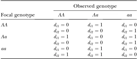
often employed (Nadaraya 1964; Watson 1964), but a trinomial kernel was adopted instead (Gianola and Van Kaam 2008), considering the three possible genotypes for every SNP. The incidence of the three genotypes can be described with two free dummy variates. Letdi1anddi2be the number of disagreements between a focal SNP combination and the observed combination in sireifor two of the three possible genotypes. In this case, the observed genotypes were AA,Aa, oraa, withAbeing the allele with the largest frequency, andd
1andd2were calculated as the sum of disagreements over loci from observing genotypes at the corresponding locus. An agreement was coded as 0, whereas a disagreement was coded as 1. Table 1 illustrates the values thatd1andd2 take at a given locus for each of the nine possible combinations of observed and focal genotypes. The trinomial kernel function had the formKh1;h2ðxxiÞ ¼h1di1h di2
2 ð1h1h2Þ2qdi1di2;
where x is the focal genomic combination and xi is the
observed genomic combination in sire i. The smoothing parametersh1 andh2 take values in the interval (0, 1) and also satisfy 0,h11h2,1 so thatKh1;h2ðxxiÞ is a suitable
candidate kernel. The EGV for each sire was the nonparamet-ric estimate using its corresponding genomic configuration as a focal point. The smoothing parameters (h1,h2) were tuned using the generalized (direct) cross-validation method de-scribed in Wahba et al. (2002). For simplicity, a single pa-rameterh1¼h2¼hwas tuned.
A Java code application was developed for computing the kernel regression on SNPs, which is available from the authors upon request.
Model 4—reproducing kernel Hilbert spaces regression:A second nonparametric procedure, a reproducing kernel Hilbert spaces (RKHS) regression, was used to estimate the effect of different genomic combinations on LM without making strong assumptions. A brief description of the RKHS is given here, and
additional details can be found in Kimeldorf and Wahba (1971), Wahba (1990, 1999), Mallick et al. (2005) and Gianolaand VanKaam(2008). This method assumes that distances in the Euclidean space can be represented in an isomorphic and isometric space, with a kernel matrix measur-ing distances between objects (focal points) in the Hilbert space. In our case, the focal points are the SNP genotypes of each individual, and the kernels involve the distance between objects. In these spaces, the penalized sum of squares has the form
J½gðxÞ jl
¼1
2½yXbgðxÞ9R
1½yXbgðxÞ1l 2kgðxÞ k
2 H ð1Þ
(Wahba 1990, 1999), where b is a vector of nuisance parameters, X is an incidence matrix, R is the residual covariance matrix, andgðxÞis a vector of unknown functions of SNP genotypes. The second term in this equation acts as a penalty, adding up some deviance depending on the value of the unknown parameterl. The termkgðxÞk2
His a norm under
a Hilbert space. Kimeldorfand Wahba(1971) found that the functiong(x) that minimizes (1) admits the representation
gðxÞ ¼a01
Xn
i¼1
aiKðxxiÞ;
where a¼ ½a0;a1;. . .;an9 is a vector of unknown
coeffi-cients,nis the number of sires genotyped, andKðxxiÞis a
reproducing kernel used as a basis function, possibly depend-ing on some smoothdepend-ing parameter(s) h. Since data were preadjusted in advance, effects other than the genomic combinations were not included in the model. In our implementation of RKHS, the intercepta0 was included in the model as the sole element ofb. The following exponential kernel meets the requirements of the RKHS structure,
KðxxiÞ ¼exp½ScoreðxxiÞ;
where ScoreðxxiÞwas a score of similarity between two SNPs
sequences. The score assigned to each pair of SNP sequences was based on the pairwise sequence alignment (Needleman and Wunsch1970), with some modifications. Theappendix shows the score system in detail. Contrary to the kernels used in Gianolaet al. (2006) and Gianolaand VanKaam(2008), this kernel does not need tuning smoothing parameters inside of the kernel.
Then, a matrix of kernelsKwith dimension 2003200, and with rows in the formk9i¼ KðxixjÞ
,j¼1, 2,. . ., 200, was TABLE 1
Disagreement scores for the heterozygote (di1) and homozygote
(di2) dummy variates considered in the trinomial kernel,
regarding the focal and the observed genotype
Observed genotype
Focal genotype AA Aa aa
AA di1¼0 di1¼1 di1¼0
di2¼0 di2¼0 di2¼1
Aa di1¼1 di1¼0 di1¼1
di2¼0 di2¼0 di2¼1
aa di1¼0 di1¼1 di1¼0
constructed. The matrixKis symmetric and positive definite and can be interpreted as a correlation matrix between genomic combinations. The minimizer gðxÞ of (1) can be expressed in a vectorial manner as
gðXÞ ¼
k91
.. .
k9j
.. .
k9n 2 6 6 6 6 6 6 4 3 7 7 7 7 7 7 5
a¼Ka:
Embedding this expression in (1) and considering thatb includes only an intercept, the function to be minimized becomes
J½m;ajl ¼1
2½y1mKa9R
1½y1mKa1l 2a9Ka;
wheremis a scalar common to all observations and1is a 2003 1 vector of ones. After setting the gradients with respect tom andato0(Mallicket al. 2005; Gianolaet al. 2006; Gianola and Van Kaam 2008), and noting the dependence on parametersl, the RKHS regression equations can be formu-lated in matrix form as
19R11 19R1K
K9R11 K9R1K1 1 l1K
ˆ ml ˆ al
¼ 19R1y
K9R1y
; ð2Þ
where R¼N1s2
e; recall that N¼ fnig, where ni is the
number of progeny of sirei. Equivalently, the RKHS approach can be formulated in terms of the random-effects model
y¼1m1Ka1e;
with the nonparametric coefficients (a) and the residuals as-sumed to be independently distributed asajlNð0;K1s2
aÞ andeNð0;RÞ, withs2
a¼l
1. This model was fitted within a
Bayesian framework withlunknown. Scale inverse chi-square prior distributions were assigned to s2
a and to the residual variance; i.e., s2
ayasa2x 1
ya and s 2 eyes2ex
1
ye, where ya¼4
andye¼3 were the degrees of freedom, ands2a¼0:75 and s2
e¼8:67 were the respective prior scale parameters. System (2) resembles the well-known mixed-model equations in animal breeding (Henderson 1975). In fact, additional fixed and random effects (including parametric genetic effects) can be included in the model if necessary (Gianola et al. 2006). Finally, the EGV of each sire was the nonparametric estimate of its corresponding genomic combination; i.e., gˆiðxiÞ ¼k9iaˆ,
whereaˆ is the posterior mean ofa. A Fortran-90 software was developed to implement the RKHS regression.
Model 5—Bayesian regression: An adapted version of the Bayesian regression proposed by Xu (2003) with Gaussian prior distributions assigned to markers (SNPs) was performed using 1000 SNPs randomly chosen from the whole genome. This model allows each SNP marker to have its own variance, producing differential shrinkage of marker effects. The model was
y¼Xb1e:
Here,b¼{bi} is 100031, andbiis a regression coefficient
for SNPi(i¼1, 2,. . ., 1000) assumed normally distributeda prioriasNð0;s2
iÞ, wheres 2
i is the unknown variance associated
with markeri. The elements of the incidence matrixXwith dimension equal to the number of records (n¼200) times the number of markers (p¼1000), relating regression coefficients for SNPs toy, were set up as in model 2 for additivity. The residuals e were assumed distributed as Nð0;RÞ, with R
constructed as in previous models. Details of the Markov chain Monte Carlo (MCMC) sampling method are in Xu (2003). The EGV of each sire was inferred by summing up the product of the Bayesian estimates (posterior means) of the regression coefficients, times the code of the respective genotype.
In summary, model 1 accounted for polygenic additive effects, and models 2 and 5 considered only additive effects of markers (24 and 1000, respectively). On the other hand, models 3 and 4 are expected to account for all additive and epistatic effects involving the 24 SNPs chosen. Models 1, 2, 4, and 5 were implemented using Bayesian methods via MCMC procedures, specifically the Gibbs sampler. Each of the analyses was based on a chain of 200,000 iterations, with the first 50,000 iterations discarded as burn-in. There were 15,000 samples used for posterior inference, obtained by drawing every 10th iteration from the chain following burn-in.
Model fit: After obtaining predicted transmitting abilities
(PTA) (model 1) and EGVs (models 2–5) of all sires, these were matched with the observed mortality rates (adjusted and raw progeny means) in the original data set. These averages were modeled via a local weighted regression using the PTA or the EGV as an explanatory variable, to examine whether the PTA or the EGV bore any relationship with mortality rates. Local weighted regression is a nonparametric approach to fitting curves to data on the basis of smoothing (Cleveland 1979). This method approximates the relationship between mortality rates (response variable) and the PTA or EGV estimates (explanatory variables) locally by a smooth curve based on a parametric function, using locally weighted least squares. Weights are assigned such that points close (in the Euclidean distance) to the predictor value of interest receive a higher weight. For convenience, fitting was such that one-fifth of the points in the plot were allowed to influence the smooth at each value. The regressions were computed using the R software (R Development Core Team 2007). The mean square error (MSE) for each method was calculated as the average of the squares of the differences between the actual average and the local weighted regression estimate at each point.
Predictive ability: The ability of predicting yet to be
observed mortality rates was studied by cross-validation for the four methods. Five subsets of data were generated by excluding 20% of the sire progeny means at random. The process was without replacement, so that all sires had missing values in only one of the subsets. This analysis was done for each method, using the variances and smoothing parameters estimated previously. The estimates for sires without pheno-typic records were obtained by treating the missing data via the data augmentation algorithm (Tanner and Wong 1987). Thus, each sire had a PTA or an EGV for scenarios with and without records for each of the five methods.
Correlations between predicted and observed adjusted means of the progeny of each sire were calculated for each subset and method. Also, a ‘‘global’’ correlation was calculated using the predicted values from the five subsets together. The model producing the highest correlation was regarded as the one with the best predictive ability of yet to be observed records.
RESULTS AND DISCUSSION
standardized log-transformed means had a fairly sym-metric distribution with mean 0 and standard deviation of 1, as expected. The combinations of 24 SNPs pro-duced 200 unique genotypes, so that each sire could be identified uniquely from its own genomic combination. Table 2 shows the variance estimates for models 1, 2, 4, and 5. The posterior mean estimates of the residual variance were 24.38, 29.97, 17.07, and 20.74 for models 1, 2, 4 and 5, respectively. This suggests that RKHS accounted for more variability than the parametric models. Using a larger number of markers with Bayesian regression (BR) did not reduce residual variance relative to RKHS, but it did in comparison to E-BLUP, which is supposed to account for all polygenic additive effects. The posterior mean of the sire variance for the E-BLUP model was 0.10, and the genetic variance explained by the markers (sum of the variances of the 1000 SNPs) for BR was 10 times larger (1.05). Hence, BR seemed to account for more genetic variance than E-BLUP. The heritability estimate of LM using E-BLUP was low (0.02), as expected, and it seems unlikely (on the basis of the posterior intervals) that the true value of this parameter exceeds 0.05. A slightly larger heritability (0.06) was reported by De Greef et al. (2001) for ascites-related
mortality, with even higher heritability estimates for heart-failure syndrome-related mortality (0.10), major heart–lung-related mortality (0.15), and total mortality (0.22). Janss and Bolder(2000) found a heritability
estimate of 0.12 for mortality 28 days after infection with Salmonella. However, comparisons should be done cautiously, because traits were different and the esti-mates in the present study were based on 200 sires only (e.g., note that the 95% highest posterior density regions for heritability ranged from 0.004 to 0.05). Also, esti-mates with linear models are frequency dependent. The nonparametric coefficient variance (s2
a, the reciprocal
of the smoothing parameter l) was estimated at 0.40
(0.07) with RKHS. The interpretation of this parameter is not obvious; in general, the smaller it is, the smoother
ˆ
gðxÞis (Hastieand Tibshirani1990). Model 3 (kernel
regression) does not lead to variance estimates directly. The hsmoothing parameter for kernel regression was estimated at 0.45. Comparison of these nonparametric results with those from other studies is not possible, since such methodology has not been used previously in quantitative genetics. The choice and design of kernels are of great importance in nonparametric regression, and they deserve further research for applications in genomic selection.
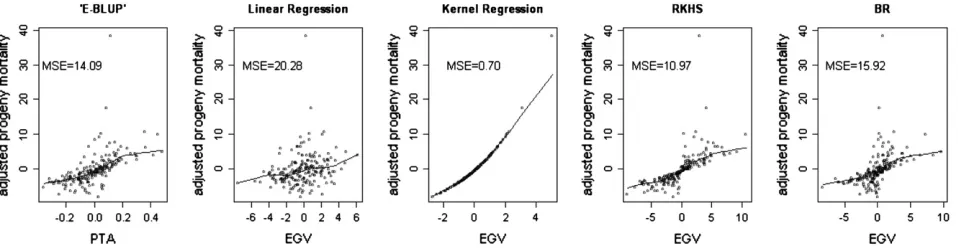
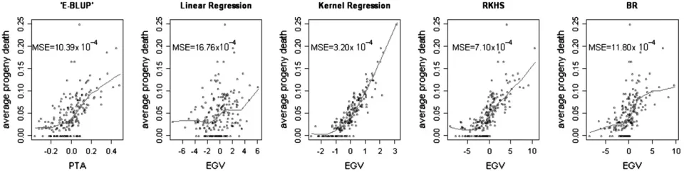
Figures 2 and 3 show the nonparametric fits relating adjusted and raw mortality in the progeny to the PTA or the EGV, respectively, for each of the five models. There was an association between PTA or EGV and progeny mortality. Sires with higher PTA or EGV had higher progeny mortality rates. Kernel regression and RKHS appeared to reproduce the data accurately, with a much smaller dispersion of average progeny LM across the regression surface than other methods. The kernel regression model fitted almost perfectly the adjusted LM (MSE ¼ 0.70; Figure 2) and produced also the smallest MSE (3.20 3104; Figure 3) with raw average progeny mortality. This is probably due to the fact that each sire had a unique marker genotype. The ranked fitted values were in exactly the same order as the ranked sire means. The nonparametric methods produced greater agreement between sire estimates and average mortality of the corresponding progeny group, and the
F‘-metric regression model fitted to the data the worst.
Predictive ability: Spearman (rs) and Pearson (rp)
correlations between estimates of sire effects from the different models ranged from 0.27 to 0.93 (Table 3). E-BLUP had a higher agreement with the BR method (rs
¼0.91,rp¼0.92) than with either kernel regression or
RKHS. This illustrates that the polygenic model
vides a close approximation to a BR model with a large number of markers having additive effects. The F‘
-metric genomic evaluation had the weakest correlations with the other methods, including the two nonpara-metric procedures, even thoughF‘, kernel regression,
and RKHS used the same information (phenotype and genomic information). This indicates that the F‘
approach produced predictions that were distinct from those from other methods. Also, E-BLUP (which does not incorporate genomic information) and the RKHS methods gave different results, and E-BLUP had a higher correlation with BR than with RKHS, as noted earlier.
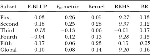
Results from the predictive cross-validation are shown in Table 4, for each of the methods. RKHS showed better predictive ability in three of the five subsets, whereas the E-BLUP and BR models were better only in one of the subsets each. RKHS had the best global predictive ability when all subsets were pooled, with the correlation being 25, 100, and 150% larger than for BR, E-BLUP, andF‘-metric, respectively. Even though LM
has a very low heritability, the RKHS incorporating
genomic information from only 24 SNPs attained better predictive ability than either E-BLUP or BR, the latter having 1000 markers in the explanatory structure. The models including genomic information had better pre-dictive ability than E-BLUP in four of five subsets (P,
0.01 under binomial sampling), and the RKHS method had a better predictive ability in three of these four subsets (P ¼ 0.05 under binomial sampling). Within methods considering genomic information, RKHS and kernel regression models can potentially account for nonadditive genetic effects (e.g., dominance and epis-tasis). The Bayesian regression did not perform better than RKHS, in spite of using a much larger amount of genomic information. This might be due to the strong assumptions placed on BR such as linearity, multivariate normality, or absence of interactions among SNPs. Further studies should deal with the inclusion of large amounts of information in the RKHS regression model and with a comprehensive comparison between meth-ods incorporating SNPs along the whole genome and those based on filtering SNP information, as in Long
et al. (2007).
Figure2.—Nonparametric locally weighted regression of adjusted progeny mortality scores on estimated sire predicted trans-mitting ability (PTA) or genomic value (EGV) for each of the five models. Mean squared errors (MSE) are given for each method. Points in the plots are the adjusted progeny average mortality for each sire. Each method led to different associations between the points and the PTA or the EGV. E-BLUP, Bayesian linear model without genomic information;F‘-metric, linear regression on SNPs based on theF‘-metric model; kernel regression, nonparametric kernel regression with SNPs within sire treated as a genomic com-bination; RKHS, reproducing kernel Hilbert spaces regression with SNPs within sire treated as a genomic comcom-bination; BR, Bayesian regression on 1000 SNPs based on Xu(2003).
TABLE 2
Posterior means (m), standard deviation (SD) (in parentheses), and highest posterior densities (HPD) regions for the residual (s2
e), sire (s 2
u), nonparametric coefficient (s 2
a), and marker (s
2
m) variances, and
heritability (h2), by model
Parameter Posterior features E-BLUP F‘-metric RKHS BR
s2
e m(SD) 24.38 (3.88) 29.97 (3.22) 17.07 (3.02) 20.74 (2.87)
HPD (95%) 16.88–32.04 24.33–36.86 11.78–23.64 15.65–26.98
Variancea m(SD) 0.10 (0.06) — 0.40 (0.07) 1.05 (0.88)
HPD (95%) 0.03–0.24 — 0.28–0.55 0.67–2.02
h2 m(SD) 0.02 (0.01) — — —
HPD (95%) 0.004–0.050 — — —
E-BLUP, Bayesian linear model;F‘-metric, linear regression on SNPs based on theF‘-metric; RKHS, repro-ducing kernel Hilbert spaces regression; BR, Bayesian regression.
aSire variance (s2
u) for E-BLUP, nonparametric coefficient variances (s2a) for RKHS, and genetic variance associated with the 1000 markers (s2
An important difference between the two nonpara-metric methods was the kernel used. Almost identical results were found when the same kernel was used in kernel regression and in RKHS; however, a trinomial kernel in RKHS would violate theoretical assumptions. Kernel regression is computationally straightforward and fast, because it can be executed without MCMC sampling. However, if some nuisance effects are to be fitted simultaneously with the marker information, a two-step method would be necessary, as described in Gianola et al. (2006), increasing computational time
and software complexity. On the other hand, RKHS is methodologically and computationally self-contained.
Nonparametric methods are expected to have a better predictive ability than parametric models when relation-ships between variables are cryptic. However, the in-terpretation of parameters is not straightforward, or even useful, since the focus is on description and prediction. A low heritability and the categorical nature of LM provided a challenge to all methods, but there was some advantage for the RKHS approach using genomic information. Bootstrapping might give a clearer picture of the uncertainty about differences in predictive abil-ity between methods. However, it is computationally demanding.
Legarraet al. (2007) found that methods
incorpo-rating genomic information had better predictive ability than BLUP in a model with independent families. In a simulation, Gianola et al. (2006) found that RKHS
regression had higher accuracy of prediction of geno-typic values than linear random regressions, mainly under additive3additive epistasis. Also, these authors assumed a different penalty structure for the nonpara-metric coefficients and used a Gaussian kernel. The kernel and scoring system developed in this study performed better than the kernel described in Gianola
et al. (2006) (results not shown).
Other authors have proposed parametric methods for including genomic information into genetic
evalua-tions. For instance, Meuwissenet al. (2001) compared
least-squares, BLUP, and two Bayesian methods with different prior distributions for the QTL effects, using simulated data. They found that Bayesian methods as-signing specific prior distributions to marker effects were more reliable, but their priors matched the sim-ulated parameter values. Also, Gianolaet al. (2003) and
Xu(2003) dealt with markers over the entire genome to
estimate polygenic effects by applying Bayesian meth-ods. Strong assumptions are needed for these methods, as mentioned earlier.
Pedigree and genomic information were not com-bined in any of the methods used in this study, due to the small number of sires. However, including both sources of information in analyses with a larger amount of data might improve predictive ability of the methods presented here.
Implications:Three methods using information from 24 SNPs associated with chicken mortality in broilers,
Figure3.—Nonparametric locally weighted regression of raw progeny mortality rate on estimated sire predicted transmitting ability (PTA) or genomic value (EGV) for each of the five models. Mean squared errors (MSE) are given for each method. Points in the plots are the raw progeny average mortality rate for each sire. Each method led to different associations between the points and the PTA or the EGV. E-BLUP, Bayesian linear model without genomic information;F‘-metric, linear regression on SNPs based on theF‘-metric model; kernel regression, nonparametric kernel regression with SNPs within sire treated as a genomic combination; RKHS, reproducing kernel Hilbert spaces regression with SNPs within sire treated as a genomic combination; BR, Bayesian regres-sion on 1000 SNPs based on Xu(2003).
TABLE 3
Spearman (above diagonal) and Pearson correlations (below diagonal) between estimates of sire effects
from the five different methods
E-BLUP F‘-metric Kernel RKHS BR
E-BLUP — 0.44 0.77 0.84 0.91
F‘-metric 0.48 — 0.33 0.36 0.46
Kernel 0.66 0.27 — 0.93 0.76
RKHS 0.84 0.36 0.79 — 0.85
BR 0.92 0.50 0.58 0.80 —
which is a lowly heritable trait, and one method using 1000 SNPs across the whole genome were used for ge-nomic evaluation of late mortality. Comparison of these methods against a standard genetic evaluation using pedigree information indicated that predictive ability was similar for E-BLUP, LM, kernel regression, and BR, but RKHS increased predictive correlations by 0.04 over BR, by 0.10 over E-BLUP, and by 0.12 over a linear regression on SNPs using the F‘-metric model. The
kernel regression and the RKHS procedure fitted the data better than E-BLUP, BR, orF‘-metric, producing a
smaller MSE. It seems that incorporating information on SNPs into genetic evaluation is feasible with non-parametric models, with the RKHS being appealing, because of its ability to deal with complex gene action as well as include parametric components in the model (Gianolaand VanKaam2008). Further, RKHS had the
highest accuracy when predicting performance of sires without progeny records in the analysis. This study suggests that RKHS using just some SNPs having an association with the trait may provide better predictive ability than a BR using markers over the entire genome. This is an important issue in the development of genomic selection procedures that must be considered in future studies in a thorough manner.
Nonparametric methods for incorporating genomic information into genetic evaluations should be studied further, since they are appealing for handling large numbers of SNPs and their interactions. At present, SNP chip developments allow genotyping thousands of SNPs for many individuals. If these methods prove to be better than existing ones, breeding companies could genotype candidates and make earlier decisions on breeding pro-grams and progeny testing, with the potential for in-creasing the rate of genetic progress (Schaeffer2006).
Developing suitable kernels to measure the extent by
which haplotypes differ from each other and that allow for weighting the most relevant SNPs differentially constitutes an important research challenge.
Useful comments made by Jan-Thijs van Kaam and Gustavo de los Campos are appreciated. Research was supported by National Science Foundation grant DMS-044371 to Daniel Gianola and by Aviagen Ltd.
LITERATURE CITED
Cleveland, W. S., 1979 Robust locally weighted regression and
smoothing scatterplots. J. Am. Stat. Assoc.74:829–836.
deGreef, K. H., L. L. Janss, A. L. J. Vereijken, R. Pitand C. L.
Gerritsen, 2001 Disease-induced variability of genetic
correla-tions: ascites in broilers as a case study. J. Anim. Sci.79:1723–1733. Gianola, D., and J. B. C. H. M.vanKaam, 2008 Reproducing kernel
Hilbert spaces regression methods for genomic assisted predic-tion of quantitative traits. Genetics178:2289–2303.
Gianola, D., M. Perez-Encisoand M. A. Toro, 2003 On marker
assisted prediction of genetic value: beyond the ridge. Genetics
163:347–365.
Gianola, D., R. L. Fernandoand A. Stella, 2006 Genomic-assisted
prediction of genetic value with semiparametric procedures. Ge-netics173:1761–1776.
Hastie, T. J, and R. J. Tibshirani, 1990 Generalized Additive Models.
Chapman & Hall, London.
Hayes, B., J. Laerdahl, D. Lien, A. Adzhubei and B. Høyheim,
2004 Large scale discovery of single nucleotide polymorphism (SNP) markers in Atlantic Salmon (Salmo salar). AKVAFORSK, Institute of Aquaculture Research, Aas, Norway. www.mabit.no/ pdf/hayes.pdf.
Henderson, C. R., 1975 Best linear unbiased estimation and
predic-tion under a selecpredic-tion model. Biometrics31:423–447. Janss, L. L. G., and N. M. Bolder, 2000 Heritabilities of and genetic
relationships between salmonella resistance traits in broilers. J. Anim. Sci.78:2287–2291.
Kimeldorf, G., and G. Wahba, 1971 Some results on
Tchebychef-fian spline functions. J. Math. Anal. Appl.33:82–95.
Lamont, S. J., M. G. Kaiserand W. Liu, 2002 Candidate genes for
re-sistance toSalmonella enteritidiscolonization in chickens as detected in a novel genetic cross. Vet. Immun. Immunopathol.87:423–428. Legarra, A., J. M. Elsen, E. Manfredi and C. Robert-Granie,
2007 Validation of genomic selection in an outbred mice pop-ulation. Proceedings of the 58th Annual Meeting of European Association for Animal Production, August 26–29, 2007, Dublin, Ireland, Session 18, Abstract 1071.
Liu, H. C., H. H. Cheng, V. Tirunagaru, L. Soferand J. Burnside,
2001 A strategy to identify positional candidate genes confer-ring Marek’s disease resistance by integrating DNA microarrays and genetic mapping. Anim. Genet.32:351–359.
Long, N., D. Gianola, G. J. M. Rosa, K. Weigeland S. Avendan˜ o,
2007 Machine learning classification procedure for selecting SNPs in genomic selection: application to early mortality in broilers. J. Anim. Breed. Genet.124(6): 377–389.
Mallick, B. K., D. Ghoshand M. Ghosh, 2005 Bayesian
classifica-tion of tumours by using gene expression data. J. R. Stat. Soc. B
67:219–234.
Meuwissen, T. H. E., B. J. Hayesand M. E. Goddard, 2001
Pre-diction of total genetic value using genome-wide dense marker maps. Genetics157:1819–1829.
Nadaraya, E. A., 1964 On estimating regression. Theor. Probab.
Appl.9:141–142.
Needleman, S. B., and C. D. Wunsch, 1970 A general method
ap-plicable to the search for similarities in the amino acid sequence of two proteins. J. Mol. Biol.48:443–453.
R DevelopmentCoreTeam, 2007 Statistical Computing.R
Founda-tion for Statistical Computing. Vienna. http://www.R-project.org. Schaeffer, L. R., 2006 Strategy for applying genome-wide selection
in dairy cattle. J. Anim. Breed. Genet.123(4): 218–223. Silverman, B. W., 1986 Density Estimation for Statistics and Data
Anal-ysis.Chapman & Hall, London.
Sorensen, D. A., and D. Gianola, 2002 Likelihood, Bayesian and
MCMC Methods in Quantitative Genetics, pp. 588–595. Springer-Verlag, New York.
TABLE 4
Pearson correlations between predicted and actual values of the progeny average of each sire for late mortality in each
subset (20% sires predicted in each subset) and by method
Subset E-BLUP F‘-metric Kernel RKHS BR
First 0.03 0.26 0.05 0.27a 0.13
Second 0.18 0.25 0.28 0.37 0.12
Third 0.18 0.13 0.06 0.01 0.17
Fourth 0.04 0.12 0.13 0.28 0.15
Fifth 0.17 0.06 0.23 0.15 0.25
Global 0.10 0.08 0.14 0.20 0.16
E-BLUP, Bayesian linear model without genomic informa-tion;F‘-metric, linear regression on SNPs based on theF‘ -metric model; kernel, nonpara-metric kernel regression with SNPs within sire treated as a genomic combination; RKHS, re-producing kernel Hilbert spaces regression with SNPs within sire treated as a genomic combination; BR, Bayesian regres-sion on 1000 SNPs based on Xu(2003).
aHigher values indicate more accurate predictions. The
Tanner, M. A., and W. H. Wong, 1987 The calculation of posterior
distributions by data augmentation. J. Am. Stat. Assoc.81:82–86. VanDerVeen, J. H., 1959 Tests of non-allelic interaction and
link-age for quantitative characters in generations derived from two diploid pure lines. Genetica30:201–232.
Varona, L., D. A. Sorensenand R. Thompson, 2007 Analysis of
lit-ter size and average litlit-ter weight in pigs using a recursive model. Genetics177:1791–1799.
Wahba, G., 1990 Spline Model for Observational Data.Society for
In-dustrial and Applied Mathematics, Philadelphia.
Wahba, G., 1999 Advances in Kernel Methods: Support Vector Machines,
Reproducing Kernel Hilbert Spaces and the Randomized GAVC, edited by B. Scholkopf, C. Burgesand A. Smola, pp. 68–88. MIT Press,
Cambridge, MA.
Wahba, G., Y. Lin, Y. Leeand H. Zhang, 2002 Optimal properties
and adaptive tuning of standard and non-standard support vec-tor machines, pp. 125–143 inNonlinear Estimation and Classifica-tion, edited by D. Denison, M. Hansen, C. Holmes, B.
Mallickand B. Yu. Springer, New York.
Wang, C. S., J. J. Rutledgeand D. Gianola, 1993 Marginal
infer-ences about variance components in a mixed linear model using Gibbs sampling. Genet. Sel. Evol.25:41–62.
Wang, C. S., J. J. Rutledgeand D. Gianola, 1994 Bayesian analysis
of mixed linear models via Gibbs sampling with an application to litter size in Iberian pigs. Genet. Sel. Evol.26:91–115. Wang, J., X. He, J. Ruan, M. Dai, J. Chenet al., 2005 ChickVD: a
sequence variation database for the chicken genome. Nucleic Acids Res.33:D438–D441.
Watson, G. S., 1964 Smooth regression analysis. Sankhya Ser. A26:
359–372.
Wong, G. K., B. Liu, J. Wang, Y. Zhang, X. Yanget al., 2004 A
ge-netic variation map for chicken with 2.8 millions single nucleo-tide polymorphism. Nature432:717–722.
Xu, S., 2003 Estimating polygenic effects using markers of the entire
genome. Genetics163:789–801.
Ye, X., S. Avendan˜ o, J. C. M. Dekkersand S. J. Lamont, 2006
Asso-ciation of twelve immune-related genes with performance of three broiler lines in two different hygiene environments. Poult. Sci.85:1555–1569.
Zeng, Z. B., T. Wangand W. Zou, 2005 Modeling quantitative trait
loci and interpretation of models. Genetics169:1711–1725. Communicating editor: J. B. Walsh
APPENDIX
A score system was developed to account for differ-ences between two sequdiffer-ences of SNPs observed in two individuals (or between a focal point and an observed genotype). This score was used as argument in the
exponential kernel employed in the reproducing kernel Hilbert spaces model. The scoring was based on a pro-cedure described by Needlemanand Wunsch(1970),
who used an algorithm to search for similarities in the amino acid sequence of two proteins. The procedure was modified and adapted to search similarities in a se-quence of SNPs within chromosomes. The score was calculated using a dynamic programming algorithm described next.
Letxiandxjbe two sequences of SNPs within a given
chromosome, with the SNPs sorted in ascending order regarding their position in the chromosome. First, calculate the frequencies (fsk) at locussof genotypek
(with k ¼ 1, 2, or 3 being one of the three possible genotypes,i.e.,AA,Aa, oraa). Then, initialize the score
S¼0. The algorithm for scoring similarity between two sequencesiandjis computed fromsgoing from 1 to the number of SNPs in a given chromosome as
if SNPsi¼SNPsj0subscore¼subscore3fsk
SNPsi6¼SNPsj0S¼S1subscore; subscore¼1:
Above, S is the score for the similarity of two sequences of SNP in a given chromosome, and subscore is a temporary variable in the algorithm that is initialized to 1 at the beginning of the algorithm and every time the sequences differ in their genotypes. The final score between both sequences is given by the sum of the scores for each chromosome as
ScoreðxxiÞ ¼
X
no:chromosomes
chr¼1
Schr:
The lower the score, the more similar the SNP sequences are. Further, the more uncommon SNPs two sequences share, the lower the score is. This score was
introduced in the exponential kernel as
KhðxxiÞ ¼exp½ScoreðxxiÞ, so that the more