Resource
Allocation
through
Goal Programming
KENNETH E. BOTTOMS AND E. T. BARTLETT
Highlight: One of the major weaknesses of using linear programming in natural resource management is that only a single criterion for determining the optimal strategy is allowed. A goal programming model is presented that allows for multiple, conflicting goals. Results are provided for a management area in northern Colorado. The trade offs between goals are demonstrated by comparison of results from multiple runs in which the order of goal preferences is varied. Goal programming is shown to be a very flexible decision aiding tool which can handle any decision problem formulated by linear programming more efficiently.
Public pressure and limited quan- tities of natural resources necessitate development of more reliable decision making techniques. Modern natural resource managers are rapidly be- coming aware of new decision aiding techniques which are capable of re- viewing, utilizing, and organizing vast quantities of resource data.
During the past decade, many models utilizing operation research techniques have been developed to aid range and other resource managers. To date, the most common technique used has been linear programming (Nielsen et al., 1966; McConnen et al., 1965; D’Aquino, 1974; Bartlett et al., 1974).
Decision makers realize, however, that linear programming models are single objective or single goal systems; the objective has commonly been prof- it maximization or cost minimization. Organizations seldom have a single goal; in fact, in public land manage-
Authors are research associate and assistant professor, Department of Range Science, Colorado State University, Fort Collins 80523.
This research is supported by NSF Grant No. ESR72-03396-A02 to the Regional Systems Program at Colorado State Uni- versity. Paper presented at the 27th Annual Meeting, Society for Range Management, Tucson, Arizona, February 3-8, 1974.
The authors wish to acknowledge the assistance of the following people for manu- script review: Dr. C. Wayne Cook, Dr. Donald A. Jameson, and Dr. David R. Betters.
Manuscript received December 11, 1974.
ment, the classical economic objective of maximum net revenue often rates only a low priority. Linear pro- gramming has been modified in order to allocate resources when multiple conflicting goals are present (Charnes and Cooper, 1961). The procedure is called goal programming.
The traditional method of solving multiple goal problems has been to define all goals in a common unit (usually dollars). Managers and most economists have been highly critical of this procedure as all goals cannot be translated into strictly economic terms. In goal programming, there is no requirement that the objectives be defined in the same value, terms. In fact, multiple goals may be in terms of board feet of timber, number of cattle, or dollars, as well as number of sales and regional incomes.
The only requirement in goal pro- gramming is that the manager can attach ordinal priorities or rankings to the goals that reflect the importance of each goal. For example, if the manager has two goals, (1) red meat production and (2) economic efficien- cy, he must rank one above the other before using goal programming. Once goals have been defined and ranked according to importance, a solution via goal programming can be obtained. The decision maker can then change the goal priorities, and by examining the solutions, he can obtain an esti- mate of the trade offs between goals.
The general logic of goal pro- gramming will be discussed, and the application t 0 natural resources explained. A discussion of an application to a forest in northern Colorado has been completed. The results of the goal program have been compared to the results of a linear program.
Goal Programming
The concept of goal programming evolved as a result of unsolvable linear programming problems and the occur- rence of conflicting multiple goals. Many allocation decisions arise in natural resource management because demands on the resource base exceed the supply capability of the eco- systems. In such instances, a linear programming model such as that de- veloped by D’Aquino (1974) will provide the manager with three words, “no feasible solution.” Goal pro- gramming will provide solutions to infeasible linear programs. In fact, the basic concept of goal programming is “whether goals are attainable or not, an objective may be stated in which optimization gives a result which comes ‘as close as possible’ to the indicated goals” (Lee, 1972). Goal programming provides the manager with estimates of achievement or non- achievement of his defined and ranked goals.
A simple example is needed to explain goal attainment. Let us assume a manager wanted to carry as close to 500 cow-calf units as possible on his ranch. Goal programming allows either overachievement or underachievement, depending on the particular decision problem. Overachievement would be any point above the 500 level, and underachievement, any point below this level. The objective of goal pro- gramming is to minimize the non- achievement of each actual goal level. If nonachievement is minimized to zero, the exact attainment of the goal has been accomplished. Using the example above, the manager might be concerned with minimizing the under- achievement, while overachievement might be more than acceptable and therefore not minimized.
the decision maker. In problems with more than one goal, the manager must rank the goals in order of importance. The procedure is to minimize the deviational variables of the highest priority goal, and proceed to the next lower goal. Deviation from this goal is then minimized with the additional constraint that attainment of the first goal cannot be lessened. The other goals are considered in order of priority but lower order goals are only achieved as long as they do not detract from the attainment of higher priority goals. Several solutions can be obtained by changing the priorities in order to indicate how the order of the goals affect planning strategies.r,.2
The goal programming model formulation used was a modification of the one developed by D’Aquino (1974). The difference between the two model formulations, of course, concerns the goals. D’Aquino’s model was composed of constraints and a single objective function, in contrast to the goal programming formulation, which contains constraints and multiple objective functions.
Since goal programming requires that each goal be assigned an impor- tance level, the concept results in a multiple objective function wherein the number of objectives is equal to the number of importance levels. Each goal does not, however, result in a separate objective function. If two or more goals can be expressed in the same units of measure, they can be within the same importance level. Dollars of budget and dollars of profit can therefore be represented in the same importance level.
In order to minimize either under- or overachievement of a particular goal, a variable called a “deviational variable” is assigned to the goal. This variable represents the magnitude by which the goal level is not achieved. If the value of the deviational variable is small, the goal is more nearly achieved than if the value is relatively large. Thus, the value of the deviational variable is minimized in an attempt to achieve the goal. Optimality occurs
’ Readers desiring an indepth discussion of goal programming should refer to Goal Bogramming for Decision Analysis by Sang M. Lee.
ZAdditionally REACT II-A Goal Program- ming Computer Program is available from the RANN Project, Department of Range Science, Colorado State University.
JOURNAL OF RANGE MANAGEMENT 28(6), November 1975 443
-
Scala in Miles
NOR lli MICHIGAN
CREEK STATE RECREATI
5 1
COLORADO
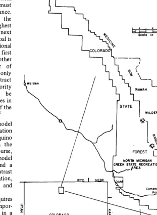
Fig. 1. The geographic location of the Colorado State Forest.
when the deviational variables of the different goals have been minimized to the smallest possible value in order of importance.
Study Area
Goal programming was applied to a resource decision problem on the mountainous Colorado State Forest, located in northern Colorado (Fig. 1). The area is approximately 9,050 acres of the southern portion of the State Forest, which ranges in elevation from 8,500 feet to over 11,000 feet. The area has been, and may increasingly become, a conflict area due to its location and its basic resource compo- sition.
Winter may begin the last of August and continue through May. Therefore, resource use is concentrated in the 3-month period from June to August.
Average precipitation ranges between 18 and 21 inches annually, with most precipitation falling as snow.
Soils in this area vary greatly but are composed mostly of granitic residues on shale or slate. Soil depth varies from 15 to 25 inches. Most of the forest soils are very susceptible to slippage and tend to be somewhat acidic. Soils in this area are very susceptible to erosion; when used intensively, great care should be taken to prevent the potential erosion.
Vegetation of the study site is extremely diverse and can be broken into several distinct types: willow carrs
and marshy meadows, grassland
meadows, sage brush meadows,
Table 1. Acreage by major vegetative types.
Vegetative type Grassland meadows Sagebrush meadows Spruce-fir
Lodgepole pine Willow bottomland
Sagebrush-lodgepole ecotone Total acres
Area (acres)
1950 2000 1450 2600 570 480 9050
Lakes cover an additional 82 acres with approximately 10.4 miles of streams. The major streams are the North Fork of the North Michigan River, its tributaries, and Grass Creek. The annual discharge from the ap- proximately 18-square-mile area of this watershed is nearly 12,500 acre feet. Sedimentation also occurs and an average production of 7.5 tons/acre/ year is considered a reasonable limit.
Recreational resources are many. The 66-acre North Michigan Reservoir along with several miles of trout stream provides a varied trout fishery, including cutthroat, rainbow, and brook trout. Camping also accounts for a significant portion of the recre- ational use, in addition to hiking and backpacking.
The timber resource at present is
capable of yielding approximately 1,275 cubic feet of lodgepole pine and 200 cubic feet of spruce-fir per acre in each of the respective ecosystems.
Results of pellet group counts give estimates of deer and elk populations that range between .12 and .15 days use per acre, which is typically related to total deer and elk population levels. Considering only areas on the site that are believed to be valuable to deer and elk, it was thought that approximately SO-60 deer and 50-60 elk frequent the area during the available season of 150 days.
Model Formulation
Several products have been identi- fied on the study area: cow-calf months of grazing, steer months of grazing, recreation user days of camping, board feet of lodgepole pine and spruce-fir timber, and deer and elk months of grazing. Each of the products is derived from one or more of the seven available resources of the study area: domestic forage, phos- phorus, protein, wildlife forage, fish, lodgepole pine, and spruce-fir, Table 2 outlines the quantities of the resources needed to produce one unit of each
Table 2. Quantities of resources needed to produce one unit of each product.
product. These values are based on the best available research results for areas similar to the study area.
Within each of the six vegetation types, several management alternatives have been defined, each of which would be expected to change the levels of production and some of the re- sources. Estimates of the expected effect of the management alternatives of the yields of the various resources for each of the vegetation types, to- gether with projected unit costs, are summarized in Tables 3 through 8. These estimates were based either on existing data in the area or research conducted on similar areas (Morrison, 1949; Stoddart and Smith, 1955; Vallentine, 197 1; and Cook, 1968). The rates for the recreation user days were calculated on an opportunity cost basis in which the acreage was assumed used for recreational purposes and therefore removed from other resource production.
No n-product-oriented goals in Table 9 were identified for manage- ment. Goals as used here became linear equations, each of which must be composed of homogeneous units al-
Products
Cow-calf Steer Recreation MBF Deer Elk
months of months user days lodgepole MBF months months
Resources grazing of grazing of camping pine spruce-fir of grazing of grazing
Domestic forage (lb) * 1209 776 0.042 753. 3080.
Phosphorus (lb) ** 2.51 1.55
Protein (lb)** 141.4 77.6
Wildlife forage (lb) * 0.057 5270 5133
Fish (lb) 1.5
Lodgepole pine (bd ft) 1000.
Spruce-fir (bd ft) 1000.
Revenue ($) 5.40 4.50 174. 408.
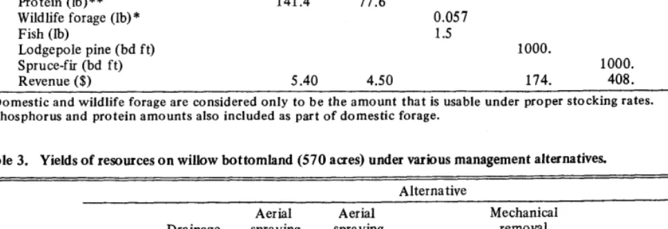
*Domestic and wildlife forage are considered only to be the amount that is usable under proper stocking rates. **Phosphorus and protein amounts also included as part of domestic forage.
Table 3. Yields of resources on willow bottomland (570 acres) under various management alternatives. Alternative
Resources
No action
Drainage of wet
lands
Aerial Aerial spraying spraying of willow with grass
land seeding
Mechanical removal
Size of action 1.0
Sediment 2.5
Domestic forage 1270.0
Phosphorus 2.54
Protein 94.0
Wildlife forage 1500.0 Fish
1.0 1.0 1.0 1.0
6.5 5.0 4.35 9.5
1459.0 647 .O 1730.0 1786.0
2.92 3.30 3.46 3.57
108.0 122.0 128.0 132.0
975.0 150.0 75.0 750.0
Recreation
Variable cost 0.00 125.00 3.50 8.50 25 .OO 25.50 6.00
Mechanical removal with grass
seeding
2 1.0 8.5 249.0 4.50 161.0 375.0
Fertili- Campground zation develoument Units _
1.0 2.0 2006.0 4.01 148.0 1875.0
3.0 Acres 27.0 Tons/acre/year
Pounds/acre Pounds/acre Pounds/acre 2250.0 Pounds/acre 2000.0 Pounds stocked/
year 1750.0 User days 2700.0 Dollars/unit
action
Table 4. Yields of resources on sagebrush vegetation type (2,000 acres) under various management alternatives,
Alternative
Mechanical Mechanical Aerial
removal removal spraying Spraying
No Mechanical with grass grass seeding Aerial with grass grass seeding, Grass
Resources action removal seeding fertilization spraying seeding fertilization interseeding units
Size of action 1.0 1.0 1.0 1.0 1.0 1.0 1.0 1.0 Acres
Sediment 9.75 10.0 9.25 7.00 5.75 5.5 5.0 6.5 Tons/acre/year
Domestic forage 825 .O 1918.0 2475 .O 2681.0 1031 .o 1116.0 125 6.0 947.0 Pounds/acre
Phosphorus .99 2.30 2.97 3.22 1.24 1.34 1.51 1.14 Pounds/acre
Protein 33.8 78.7 161.0 110.0 42.3 45.7 51.5 38.8 Pounds/acre
Wildlife forage 2500.0 1000.0 875.0 750.0 1500.0 1375 .o 1125.0 2375 .O Pounds/acre
Variable cost 0.00 15.00 17.50 32.50 3.00 18.00 20.50 7.50 Dollars/unit
action
though the units may differ between goals. The goal level is the amount of each goal unit desired, such as number of cow months, board feet of timber, acre feet of water, etc.
The initial results indicate that goal programming will mimic the linear programming solution if the objective function of the linear program is the lowest priority goal or if only one objective is considered in the goal program. Conventional linear pro- gramming requires all constraints be met before profit is maximized. The same requirement must be made of goal programming before it can mimic linear programming. Setting all goals at a higher priority than the linear pro- gramming objective or only using one objective accomplishes the same end. The goals, goal levels, and priorities are shown in Table 9. In the linear pro- gram, profit maximization was the objective function and the remaining eight goals were entered as minimum constraint requirements.
The results from the linear and goal programs were identical with all goals being met or exceeded. The number of steers and amount of lodgepole pine and spruce-fir timber were exceeded
Table5. Yields of resources on sagebrush-lodgepole ecotone (480 acres) under various management alternatives.
Alternatives
Wildlife Campground habitat
Resources No action development development Units
Size of action 1.0 3.0 1.0 Acres
Sediment 5.65 25.35 9.82 Ton/acre/year
Domestic forage 525.0 Pounds/acre
Phosphorus .79 Pounds/acre
Protein 28.4 Pounds/acre
Wildlife forage 1418.0 2979.0 2128.0 Pounds/acre
Fish 3200.0 Pounds stodced/year
Recreation 2700.0 User days
Variable cost 0.00 25 00.00 35 0.00 Dollars/unit action
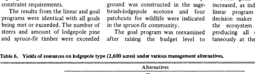
because of the contribution to the objective function of the linear pro- gram or the profit goal in the goal program. The ecosystems produced an ample amount of wildlife forage; con- sequently, animal numbers exceeded the minimum. With two exceptions the ecosystems were managed under the “no action” alternative. One camp- ground was constructed in the sage- brush-lodgepole ecotone and four patchcuts for wildlife were indicated in the spruce-fir community.
The goal program was reexamined after raising the budget level to
$90,500 and then to $135,750 (Table 9). Profit increased as a result of an increase in spruce-fir production and a slight increase in steers without an increase in cows. The only change in the management alternatives was an increase in the number of patchcuts in the spruce-fir ecosystem.
Some goals of the model were increased, as indicated in Table 10. A linear program will not aid the decision maker in this case, because the ecosystem is not capable of producing all of the goals simul- taneously at the given budget levels.
Table 6. Yields of resources on lodgepole type (2,600 acres) under various management alternatives.
Alternatives
Resources No action
Clearcut harvest
Clearcut replant nursery stock
Patch cutting
Campground
development units Size of action
Sediment Domestic forage Phosphorus Protein Wildlife forage Fish
Recreation Lodgepo le pine Variable cost
1.0 1.0 1.0 40.0
6.5 9.05 7.65 350.0
225 .O 786.0 28064.0
.38 1.34 47.6
15.0 52.6 1880.0
337.0 565.0 168.0 26941.0
562.5 11250.0 14062.0 18000.0
0.00 400.00 489.00 11000.00
3.0 27.75
606.0 1500.0 2000.0 2700.00
Acres Tons/acre/year Pounds/acre Pounds/acre Pounds/acre Pounds/acre Pounds sto eked/year User days
Board feet Dollars/unit action
Table 7. Yields of resources on spruce-fir type (1,450 acres) under various management alternatives.
Alternatives
Resources No action Clearcut
Size of action Sediment Domestic forage Phosphorus Protein Wildlife forage Fish
Recreation Spruce-fir Variable cost
1.0 1.0
7.0 9.25
40.0 1.0
0.39 0.78
15.4 30.9
125.0 200.0
350.0 7000.0
0.00 452.00
Clear cut
replant Selective Patchcut Campsite
nursery stock cut for wildlife development Units
;:!: 9.75 1.0 350.00 40.0 28.5 3.0 Acres Tons/acre/year
348.0 14744.0 Pounds/acre
0.59 25.2 Pounds/acre
23.2 988.0 Pounds/acre
100.0 250.0 12480.0 112.5 Pounds/acre
1200.0 Pounds stocked/year
500.0 User days
7700.0 2100.0 280000.0 Board feet
5 10.00 376.00 10000.00 2700.00 Dollars/unit action
Table 8. Yields of resources on grassland type (1,950 acres) under various management alternatives.
Resources No action Interseeding
Disking and Disk, interseed
interseeding and fertilizer Disk Units
Size of action 1.0
Sediment 1.5
Domestic forage 2450.0
Phosphorus 3.92
Protein 66.2
Wildlife forage 625 .O
Variable cost 0.00
1.0 1.0 1.0 1.0 Acres
3.5 8.25 8.0 8.5 Tons/acre/year
2817.0 3062.0 3552.0 2940.0 Pounds/acre
4.51 4.90 5.63 4.7 Pounds/acre
76.1 82.7 95.9 79.4 Pounds/acre
469.0 250.0 125.00 312.0 Pounds/acre
6.50 7.95 12.45 7.00 Dollars/unit action
Table 9. Results of linear and goal programs with varying budget levels.
Results Constraint (LP) Priority for
or goal level (GP)’ goal program
Linear program
Goal programs
1 2 3
Budget 0) -
Cow-calf months of grazing 200.
Steer months of grazing 50.
Recreation user days 3,000.
Lodgepole pine (MBF) 240.
Spruce-fir (MBF) 120.
Sediment (tons) 67,875.
EIk months of grazing 50.
Deer months of grazing 25.
Profit ($) 2,000,000.
i 2 3 4
5 -
6 7 8 9
45,250. 45,250. 90,5 00. 135,750.
200. 200. 200. 200.
3,846. 3,846. 3,868. 3,890.
3,000. 3,000. 3,000. 3,000.
1,463. 1,463. 1,463. 1,463.
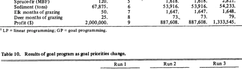
1,618. 1,618. 2,821. 4,025.
5 3,916. 53,916. 54,233. 54,549.
1,647. 1,647. 1,648. 1,649.
73., 73. 79. 85.
887.608. 887,608. 1,333,545. 1,779,481. ‘LP= linear programming; GP = goal programming.
Table 10. Results of goal program as goal priorities change.
Run 1 Goal
priority Level
Goal Goal level ranking achieved
Profit ($) 2,000,000. 1 926,337.
Cow-calf months of grazing 200. 2 0.
Steer months of grazing 50. 3 4,214.
Recreation user days 45,000. 4 0.
Lodgepole pine (MBF) 240. 5 1,463.
Spruce-fir (MBF) 120. 6 1,711.
Sediment (tons) 67,875 7 5 3929.
Elk months of grazing 500. 8 1,107.
Deer months of grazing 600. 9 600.
Budget (8) 45,250. - -
Run 2 Goal
priority Level ranking achieved
4 434,500.
2 200.
3 3,808.
1 38,613.
5 1,463.
6 508.
8’
5 3,764. 1,096.
9 600.
-
Run 3 Goal
priority Level ranking achieved
4 434300.
2 200.
1 3,808.
3 38,613.
5 1,463.
6 508.
7 5 3,764.
8 1,096.
9 600.
-
Run 4 Goal
priority Level ranking achieved
4 2,000,000.
2 200.
3 5,229.
1 45,000.
5 1,153.
6 7,759.
7 64,139.
8 1,418.
9 600.
10 1,391,089.
Conflict for scarce resources forces the manager to sacrifice some of his goals in order to meet others. Multiple runs using linear programming would not show any trade offs between goals and would be many times more expensive. In such a situation, information con- cerning the trade off between goals would greatly aid the resource manager. To provide such information, the goal programming model was solved using several different orders of goal priorities. Such varying of the order of goals will be defined as parametric goal programming.
Table 10 outlines the results of the three parametric goal programming runs, each of which has a different top priority goal. Table 10 also shows how the results differ if the budget is entered as a goal instead of a futed constraint.
Run one was based on profit max- imization as the top priority goal. Steers were favored over cow-calf units, spruce-fir over lodgepole pine with no user days produced. The only alternative other than “no action” alternatives was 4.5 forty-acre patch- cuts in spruce-fir. The profit generated was $926,337. All goals, whether com- pletely achieved or not, were met to the fullest possible extent given the priority ranking.
The second test had user day pro- duction as the highest priority goal with priority of profit dropping to fourth. User day production increased to 38,613, which is the maximum given a fixed budget of $45,250. Eighteen campgrounds were indicated on the sagebrush-lodgepole ecotone. The cow-calf goal was met in this run because profit was no longer over- riding this alternative. Steer pro- duction dropped because of recreation and the presence of cow-calves. Spruce-fir production dropped because the budget was consumed in recreation development instead of timber harvest- ing; thus no patchcuts were indicated. Table 11. Management alternatives selected
priority rather than a constraint goal.
Elk numbers decreased slightly because of the overall decrease in wildlife forage being produced on the area. The profit was approximately one-half that of the first run.
The third test had steer production as the highest goal, followed by COW-
calf, recreation, and profit. The results are the same as when recreation was the highest goal because the low goal level is met on all runs. This indicates to the manager that steer production is not a critical goal except as it relates to profit.
In the last test, the budget con- straint was changed from a constraint to the last priority goal (tenth). In this case, all levels of the other goals were met but at a cost of $1,39 1,089. This is over 30 times the budget level of $45,250. The management alternatives indicated in the solution are shown in Table 11.
Conclusions
The public ideally views the sound- ness of a decision-making process by the degree that goals are achieved by a decision. Goal programming measures the degree of goal attainment and has the ability to solve problems involving multiple conflicting goals according to an ordinal priority structure.
Goal programming enables the manager to program multi-objective problems. Goal programming is par- ticularly applicable as a planning aid to agencies such as the Forest Service and the Bureau of Land Management, where multiple resource management is essential.
The goal-programming procedure is one more tool available to natural resource decision makers. We, as resource managers, must strive to improve our decision-making processes. Any tool which can, in any way, aid the decision maker in arriving at good solutions to complex problems should be reviewed, evaluated, and used when feasible.
under the goal program with budget as a last
Model formulations have shown great promise as effective decision- aiding tools for natural resource allocation (D’Aquino, 1974; Bartlett et al., 1974). The idea of using the level of goal attainment as objective functions rather than the conventional profit or cost seems to more closely approximate the actual thinking process of the manager. Quantification of this nature sets the foundation for an iterative updating system so neces- sary if operation research tools are to be used in practical applications to natural resource allocation processes.
Literature Cited
Bartlett, E. T., G. R. Evans, and R. E Bement. 1974. A serial optimization model for ranch management. J. Range Manage. 27:233-239.
Charnes, A., and W. W. Cooper. 1961. Management models and industrial ap- plications of linear programming: I and II. John Wiley and Sons, Inc., N.Y. Cook, C. Wayne, and L. E. Harris. 1968.
Nutritive value of seasonal ranges. Utah State Univ. Agr. Exp. Sta. Bull. NO. 472, Logan. 55 p.
D’Aquino, Sandy A. 1974. Optimum al- location of resources: A programming approach. J. Range Manage. 27 : 228-233. Lee, Sang M. 1972. Goal programming for decision analysis. Auerbach Publishers Inc., Philadelphia, Pa. 387 p.
McConnen, R. J, D. K. Navon, and E. L Amidon. 1965. Efficient development and use of forest lands: An outline of a prototype computer-oriented system for operation planning, p 18-32. In Mathe- matical models in forest management. Forestry Commission, Forest Record No. 59.
Morrison, Frank B. 1949. Feeds and feeding. The Morrison Publishing Company, Ithaca, N.Y. 1207 p. Nielsen, Darwin B., William G. Brown,
Dillard H. Gates, and Thomas R. Bunch. 1966. Economics of federal range use and improvement for livestock pro- duction. Oregon Agr. Exp. Sta. Tech. Bull. No. 92. 40 D.
Stoddart, Laurence A., and Arthur D. Smith. 1955. Range management. McGraw-Hill Book Co., Inc., N.Y. 433 p. Vallentine, John F. 1971. Range develop- ments and improvements. Brigham Young Univ. Press, Provo, Utah. 516 p.
Alternative Amount
Fertilization of willow bottomland (acres) 570.
Campgrounds in sagebrush-lodgepole ecotone (3 acres) 0.
Wildlife habitat development in sagebrush-lodgepole ecotone (3 acres) 480.
Patchcut for wildlife in lodgepole pine (40 acres) 64.
CLYDE ROBIN
NATIVE SEEDSCampgrounds in lodgepole pine (3 acres) 12.3
Selective cut in spruce-fir (acres) 313.
Patchcut for wildlife in spruce-fir (40 acres) 25.
Campgrounds in spruce-fir (3 acres) 41.
Castro Valley, California 94546