Compositional Variations of Titan's Impact Craters Indicates Active Surface Erosion

(1)

Scholarship@Western

Electronic Thesis and Dissertation Repository

7-30-2018 2:00 PM

Compositional Variations of Titan's Impact Craters Indicates

Active Surface Erosion

Alyssa Werynski

The University of Western Ontario

Supervisor

Neish, Catherine D.

The University of Western Ontario Graduate Program in Geophysics

A thesis submitted in partial fulfillment of the requirements for the degree in Master of Science © Alyssa Werynski 2018

Follow this and additional works at: https://ir.lib.uwo.ca/etd

Part of the Geology Commons

Recommended Citation Recommended Citation

Werynski, Alyssa, "Compositional Variations of Titan's Impact Craters Indicates Active Surface Erosion" (2018). Electronic Thesis and Dissertation Repository. 5585.

https://ir.lib.uwo.ca/etd/5585

This Dissertation/Thesis is brought to you for free and open access by Scholarship@Western. It has been accepted for inclusion in Electronic Thesis and Dissertation Repository by an authorized administrator of

(2)

i

Impact craters on Titan are relatively scarce but provide ample information about the

subsurface properties and modification processes present there. This study utilizes impact

craters to examine compositional variations across Titan’s surface and their subsequent

modification. Fifteen craters and their ejecta blankets were studied. Subsurface composition

was inferred from emissivity data from Cassini’s RADAR instrument, and surficial composition from Cassini’s Visible and Infrared Mapping Spectrometer (VIMS). Results

show subsurface composition of these craters is controlled by their degradation state and

local environment. Older craters are more infilled with organics than younger, and dunes

craters show more organic enrichment than plains craters. Surficial composition is only

controlled by the local environment (i.e. dunes or plains regions). Since degraded craters

show organic rich subsurfaces, but varying surface compositions, it is likely there is an active

surface process clearing the surface of sediments and infilling the craters’ subsurface

fractures.

Keywords

(3)

ii

Co-Authorship Statement

Chapter 3 is a version of a manuscript for publication submission titled “Compositional

Variations in Titan’s Impact Craters Indicates Active Surface Erosion”. Co-authors are Dr.

Catherine Neish, Dr. Alice Le Gall, Dr. Michael Janssen, and the Cassini RADAR team.

Mapping techniques and the first method of analysis was completed by A. Werynski. The

second method of analysis was completed by Dr. Le Gall. Interpretations and suggestions

(4)

iii

Acknowledgments

Thank you to Dr. Catherine Neish for not only providing me with a thesis topic I thoroughly

enjoyed but also for the unconditional and helpful guidance in this work. Thank you

especially for understanding the delicate balance and intricate relationship between work and

personal life. Thank you for pushing me, supporting me, and reminding me that I can do it!

Thank you for sending me to so many different conferences – these were all truly enjoyable

and of course, educational. An additional thank you to Dr. Alice Le Gall for all of her helpful

insights and feedback in this work.

Thank you to my friends near and far who helped me through the last year whether it was

with my research, field work, or enjoying my time in London. Thanks to Lindsay especially

for kicking my writing into gear. Thanks to Jordan and Sarah (and Lindsay) for keeping me

sane and introducing me to a lot of new things. Thanks to Liam for sharing a love of sports.

And of course, thanks to Josh for his helpful MATLAB guidance whenever Mathematica

failed me.

Finally, thank you to my parents. Thank you for unconditionally supporting me in

everything I want to do – whether it be moving to a new state or country, deciding to go back

to school, or wanting to travel the world. Thank you for putting up with me and thank you

(5)

iv

List of Tables

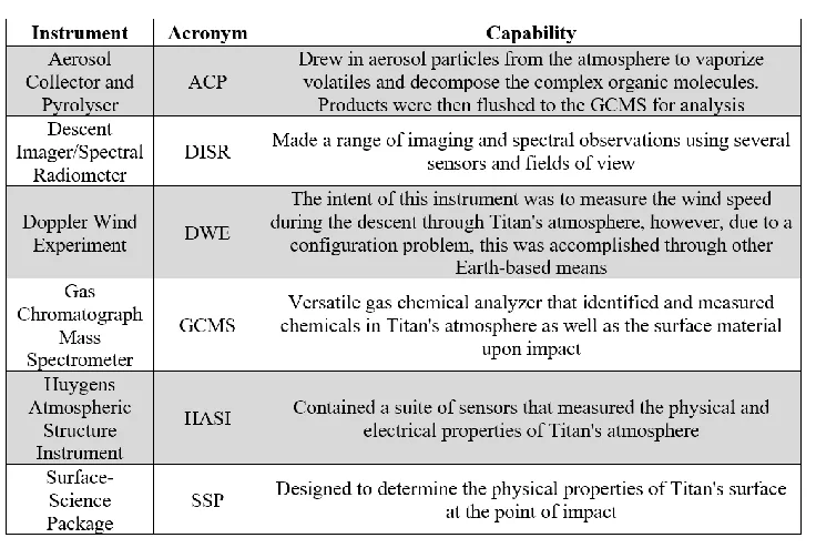
Table 1: Instrument suite for the Huygens probe... 5

Table 2: Payload suite onboard the Cassini spacecraft. ... 6

Table 3: Environmental Conditions on Titan... 7

Table 4: Relative depths for 10 craters on Titan. ... 65

Table 5: Calculated high and low resolution mean emissivity for 15 craters on Titan ... 67

(8)

vii

List of Figures

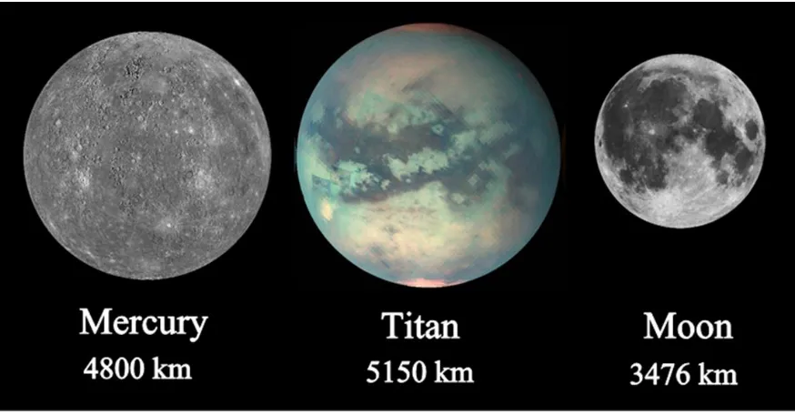
Figure 1: Size comparison of Mercury, Titan, and Earth's Moon. Approximate diameters

(km) for each body listed here. Image created from NASA's image archive. ... 2

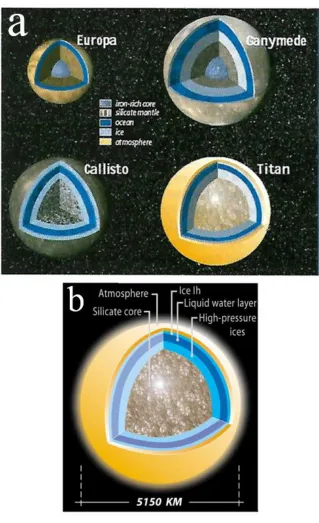
Figure 2: a) Hypothesized interior structures of the icy Galilean satellites, Europa,

Ganymede, and Callisto in comparison to Titan. Figure 2a from Sotin et al., 2009. b)

Modeled interior structure of Titan, which likely has a silicate, or mix of ice and rock, core,

surrounded by high pressure ices. Beneath the icy crust there is likely a liquid water ocean.

Figure 2b from Tobie et al., 2005. ... 3

Figure 3: Spectral plot obtained from VIMS image v1525115629_1 centered at ~32°N,

12°W. The atmospheric windows are illustrated by the wavelength peaks. ... 7

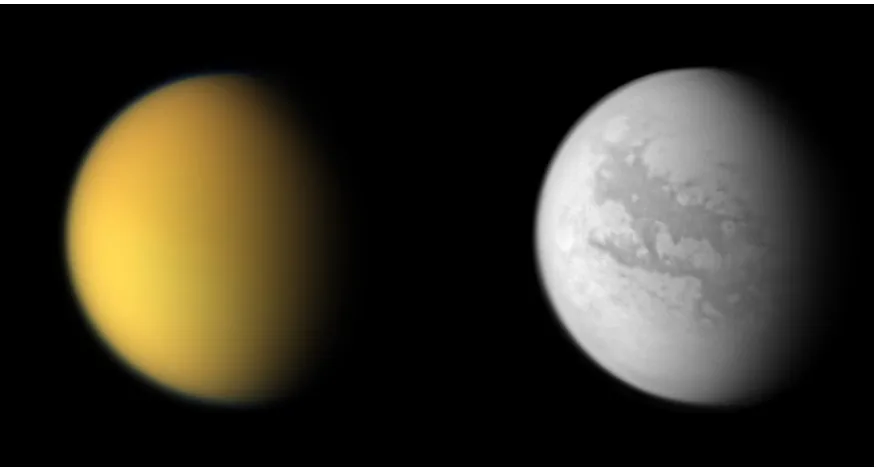
Figure 4: Titan in different wavelengths of light. The left image shows what Titan would

look like to the human eye. The right image shows a near-infrared wavelength image (0.938

µm), capable of viewing the surface (NASA, 2018). Both images were acquired by Cassini’s

Imaging Science Subsystem (ISS). ... 8

Figure 5: Map of major geomorphologic units on Titan. Labyrinth terrain represented in red,

undifferentiated plains in green, hummocky/mountainous terrain in yellow, and sand dunes in

purple. Cassini ISS map underneath available RADAR image swaths to provide context.

Image from Lopes et al., 2016. ... 9

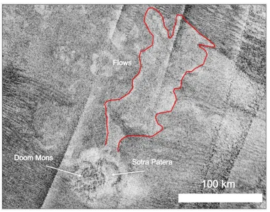
Figure 6: Radar image of potential cryovolcanic feature called Sotra Facula. Here, North is

up. A 1450 m high mountain, Dooms Mons is to the west of Sotra Patera, a 1700 m deep pit.

The associated lobate flows are outlined in red, flowing in a NE direction. ... 11

Figure 7: Cat scratch features (~16°N, 93°W) shown by the radar as dark streaks flanking the

western and eastern sides of the image. These were later determined to be longitudinal dune

features. Image from NASA’s image archive. ... 12

Figure 8: a) Visible images taken by the Huygens probe DISR showing dark, dendritic fluvial

(9)

viii

to be classified as a sea, named Ligeia Mare. These images are in polar projection (modified

from Lopes et al., 2010). ... 13

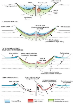
Figure 9: Series of schematic cross-sections depicting the three main stages in the formation

of simple (left) and complex (right) craters. Modified from Osinski et al., 2011. ... 15

Figure 10: Radar map of Titan with the 90 craters circled in red. The size of the circle is

proportional to the crater's diameter. Note the lack of craters near the poles. Image from

Hedgepeth et al., 2018. ... 18

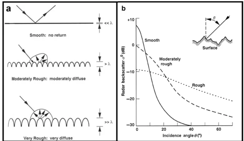
Figure 11: a) Schematic showing how a surface will scatter the radar energy in certain

directions based on the wavelength-scale roughness of its surface. b) Radar backscatter also

depends on the incidence angle of the beam. Smoother surfaces can have strong returns

when the incidence angle is close to the surface slope angle, but have very weak returns at

incidence angles greater than 30°. Image from Neish and Carter, 2014, adapted from Farr,

1993... 29

Figure 12: Cassini RADAR image of Santorini crater located at 2.2°N, 147.7°W. Radar

bright regions correspond with the rough crater rim and ejecta blanket. Radar dark regions

correspond with the smooth surrounding sand dunes and sediment infill in the crater interior.

Sand dunes appear smooth in radar because grain size is only a few hundred microns and the

radar senses surface roughness at centimeter scales. ... 30

Figure 13: The Sun’s spectrum (black) in relation to a perfect emitter, or blackbody (green),

at the same temperature. The Sun is considered a blackbody but note how the Sun’s

spectrum does not match up evenly with a laboratory spectrum of a similar temperature

blackbody. In nature, nothing is ‘perfect’, therefore objects in nature will have emissivity

values less than 1. Image from Physics Stack Exchange. ... 32

Figure 14: Global emissivity map of Titan from Janssen et al., 2016. Higher emissivities are

represented by warmer colors and indicate organic enrichment. Lower emissivity values are

represented by cooler colors and are interpreted as water-ice enrichment. ... 33

Figure 15: An example of volume scattering of sunlight on a tree top. Leaves, as well as

(10)

ix

Figure 16: Global VIMS mosaic of Titan from Cassini observations by Barnes et al., 2007.

Colors are mapped with red as 4.8-5.2 μm, green as 2.0 μm, and blue as 1.28 μm. Reds are

either clouds or evaporites, blue represents water-ice, browns are sand dunes, and green is an

unknown unit, likely a mix of organics and water-ice. Figure modified from Neish et al.,

2015... 36

Figure 17: Spectra of pure water-ice shown from a wavelength range of 0.8-3.0 microns.

Note the large absorption bands at ~1.5 and 2.0 microns (Kokaly et al., 2017). ... 37

Figure 18: VIMS spectra from 3 distinct units on Titan. a) VIMS brown spectra, indicative

of organics. b) VIMS blue spectra, indicative of a water-ice enrichment. c) VIMS green

spectra, an unknown unit, potentially a mix of water-ice and organics. ... 38

Figure 19: VIMS spectra for Sinlap crater and the surrounding region on Titan. The RGB

image shown is a band ratio image (R: 1.59/1.27, G: 2.03/1.27, and B: 1.27/1.08). Blue

regions and spectra correspond with a proposed water-ice unit, brown regions and purple

spectra are likely organic, white regions and red and black spectra represent an unknown

unit. The green spectra is derived from a single pixel and could be affected by a cosmic ray,

however, this pixel has been captured in previous images and likely represents a surface

heterogeneity. I/F is the observed spectral radiance divided by the solar irradiance (Le

Mouelic et al., 2007). ... 39

Figure 20: VIMS-IR images of the same area of Titan at 3 different wavelengths. As the

wavelength gets shorter, there are more scattering effects caused by the haze in the

atmosphere (McCord et al., 2006). ... 40

Figure 21: Surface mass to charge ratios acquired from the GCMS on board the Huygens

probe. Data was taken starting upon impact until signal was lost (Niemann et al., 2005). ... 41

Figure 22: Cassini RADAR basemap comprised of all available radar images. ... 42

Figure 23: Interpolated global elevation map of Titan obtained from Corlies et al., 2017.

(11)

x

Figure 24: Image showing process of creating the high resolution emissivity mosaic. a) The

global, low resolution, emissivity dataset for Titan. b) All high resolution, BIBQI-, radar

images of Titan. These images were acquired at the same time as the highest resolution

emissivity swatches and therefore match up with each other. c) The radar swatches shown in

b) were used to extract the emissivity data from a) to create the high resolution data product

shown here. ... 45

Figure 25: Three VIMS images with the color scheme outlined in Barnes et al., 2007

showing Sinlap crater. The highest resolution image is placed on top. The lowest resolution

is placed on the bottom, providing more context to the region. ... 47

Figure 26: Cassini RADAR map of Titan. All 15 craters in this study are shown in red and

labeled. ... 57

Figure 27: Cassini RADAR images of the 15 craters (outlined in red) studied in this work, in

order of size. North points up in all images. a) Menrva, D ~ 425 km. b) Forseti, D ~ 139 km.

c) Paxsi, D ~ 120 km. d) Afekan, D ~ 115 km. e) Hano, D ~ 100 km. f) Sinlap, D ~ 82 km.

g) Selk, D ~ 80 km. h) Soi, D ~ 78 km. i) Guabonito, D ~ 68 km. j) Nath, D ~ 58 km. k)

Unnamed crater discovered in flyby T104, D ~ 57 km. l) Momoy, D ~ 40 km. m) Ksa, D ~

39 km. n) Shikoku, D ~ 35 km. o) Santorini, D ~33 km. ... 58

Figure 28: 2.18 cm emissivity data overlain on Cassini RADAR images of the 15 craters of

interest on Titan (outlined in red), in order of size. North points up in all images. a) Menrva,

D ~ 425 km. b) Forseti, D ~ 139 km. c) Paxsi, D ~ 120 km. d) Afekan, D ~ 115 km. e)

Hano, D ~ 100 km. f) Sinlap, D ~ 82 km. g) Selk, D ~ 80 km. h) Soi, D ~ 78 km. i)

Guabonito, D ~ 68 km. j) Nath, D ~ 58 km. k) Unnamed crater discovered with flyby T104,

D ~ 57 km. l) Momoy, D ~ 40 km. m) Ksa, D ~ 39 km. n) Shikoku, D ~ 35 km. o)

Santorini, D ~33 km. ... 60

Figure 29: Available VIMS data overlain on Cassini RADAR images for 12 of the 15 craters,

outlined in red. VIMS spectra colors: blue is 1.28 µm, green is 2 µm, and red is 4.8-5.2 µm.

Blue units are water-ice, green units are an unknown unit potentially organics and water-ice,

(12)

xi

crater discovered with flyby T104 (smaller), d) Afekan, e) Sinlap, f) Selk, g) Soi, h)

Guabonito, i) Nath, j) Ksa, and k) Santorini. ... 61

Figure 30: Cassini RADAR image of Forseti crater. Radar bright regions here correlate with

the crater’s rough rim and ejecta blanket, outlined in red. The radar dark material in the crater

floor may be smooth sediments deposited there by aeolian or/and fluvial activity. A possible

central uplift as inferred from crater diameter and radar imagery is observed on the floor as

well. ... 62

Figure 31: Cassini RADAR image of Forseti crater with global emissivity data overlain. The

NE segment of the crater shows the higher resolution emissivity data available whereas the

SW segment of the crater is covered by the lower resolution data set. ... 63

Figure 32: Left: Outlines of the Forseti crater (black) and radiometry footprints (blue) over

the crater region. Right: Emissivity of the crater area as a function of the areal filling factor

by the crater rim and ejecta of each radiometry footprint and associated linear fit (solid line).

... 66

Figure 33: Mean emissivity versus (a) crater longitude (°W), (b) crater latitude and (c) crater

elevation. The dashed lines represent average global background values for the high

resolution data set in addition to the low resolution data set. Blue boxes correspond to the

low resolution data set, black circles represent the high resolution data set. ... 69

Figure 34: Mean emissivity for crater rim and ejecta blankets on Titan versus relative crater

depth. Craters with larger relative depths (more degraded) have higher emissivity than

craters with smaller relative depths (less degraded). However, composition also depends on

location. Here we see Santorini and Shikoku (dunes craters) with higher emissivities than

Soi, the most degraded crater. This will be discussed further in section 3.3.2. The arrow

indicates that this is an upper limit to Forseti’s relative depth. ... 70

Figure 35: Filling factor emissivity of the ejecta blanket + rim and the floor of 12 craters on

Titan. Cooler colors correspond with lower emissivities and warmer colors represent higher

emissivities. The crater ejecta blanket + rim and floor emissivities were obtained by

extrapolation of the emissivity for a filling factor of 100% (see section 3.2.2). There is a

(13)

xii

Santorini which have been observed with radiometry footprints including more than 50% of

other terrains. Note that, except for Sinlap, the crater floors are always more emissive than

the crater ejecta blankets + rims, most likely because these are sinks for organics. ... 72

Figure 36: Emissivity difference between crater floor and crater ejecta blanket + rim versus

relative depth. The dashed line represents an equivalent emissivity for the crater interior and

exterior. The solid blue line shows the general trend of the craters. Sinlap is the only crater

with a lower emissivity value in the interior, implying extreme youth. As craters degrade

toward intermediate ages, this difference increases. As craters become heavily degraded, this

difference becomes minimal again. ... 73

Figure 37: Top images show radar images, center images show VIMS data, bottom images

show 2.18-cm emissivity data of Sinlap, Santorini, and Soi. The ejecta of Sinlap, a dunes

region crater, exhibits a bright green VIMS spectra, potentially a mix of organics and

water-ice. The emissivity data shows a blue signature, indicative of a lower value that is interpreted

as water-ice. Santorini, a relatively degraded dunes crater, but less degraded than Soi, shows

a VIMS green spectra on its ejecta blanket. The emissivity data shows a heavily organic

region, represented by the dark red hue. The ejecta of Soi crater, a degraded plains crater,

shows VIMS dark blue unit, suggestive of water-ice. The emissivity data shows a reddish

hue, indicating a higher value or an organic-rich composition. ... 75

Figure 38: Hypothesis for the evolution of a crater in the dunes region. In the pre-impact

stage, the surface shows a brown spectra, indicative of sand dunes, and a high emissivity,

indicative of an organic-rich substrate. Immediately post-impact, a well-preserved crater is

formed. The ejecta blanket and rim shows a surficial VIMS green spectra, likely a mix of

organics and water-ice. The ejecta blanket and rim shows a water-ice rich subsurface. Over

time, as this crater degrades, the VIMS signature of the ejecta blanket remains the same due

to active surface processes, but the subsurface becomes more organic-rich as the fractures are

infilled by sediment. A similar process happens in the plains regions: the VIMS spectra

(14)

Chapter 1

1

Introduction

Impact cratering affects virtually all solid rocky and icy surfaces in the solar system. By

studying the cratering processes on different planetary bodies, more can be learned about

the process as a whole, as well as provide clues about the characteristics and exogenic

processes on the target body. Since this process affects a wide range of planetary

surfaces with various differing geologic characteristics, it is possible to learn how

different factors control the process. For instance, the effects of an atmospheric

component on the cratering process could be studied. Additionally, impact cratering

reveals valuable information about the target subsurface and its composition, something

that would otherwise remain hidden from study. Researching this process is especially

important for bodies at great distances from Earth – it is difficult and costly for missions

to reach these locations, so we must be as prepared as possible for what environments

will be encountered. For example, Saturn’s moon Titan is in the outer solar system, and

by studying its craters, we are learning that it is a dynamic place. We do not, however,

understand how craters on Titan are modified over time and what that implies about its

modification processes.

1.1 Titan

Titan was discovered by Dutch astronomer Christiaan Huygens on March 25, 1655. It

was the first Saturnian moon discovered and is the largest of Saturn’s 62 known satellites,

as well as the second largest satellite in the entire solar system. It has a mean radius of

2,576 km and is larger than the smallest planet, Mercury, which has a radius of 2,440 km

(Figure 1). The sheer grandness of Titan inspired its name, suggested by John Herschel.

Titan is tidally locked to Saturn, therefore its rotational period and orbital period are

equivalent, completing a full orbit or rotation during a period of 15.945 days (Coustenis,

(15)

Figure 1: Size comparison of Mercury, Titan, and Earth's Moon. Approximate

diameters (km) for each body listed here. Image created from NASA's image

archive.

The interior structure of Titan is believed to be somewhat similar to the icy Galilean

satellites of Jupiter (Figure 2). Callisto likely has a rocky core, surrounded by alternating

layers of ice and liquid oceans, whereas Europa likely has an iron core, a rocky shell

surrounding the core, followed by a liquid ocean layer entrapped by a shell of ice (Sotin

and Tobie, 2004). The interior of Ganymede is thought to be similar to Europa’s interior,

with the exception of an icy layer between the liquid ocean and the rock surrounding the

iron core. Titan most closely resembles the interior of Ganymede, however with

differing core compositions (Figure 2b). Titan’s core is thought to be rocky, or perhaps

an ice-rock mix, different than Ganymede’s iron core (Tobie et al., 2005). Overall, the

internal structure of Titan is poorly understood, however, recent studies (e.g. Nimmo and

Bills, 2010; Iess et al., 2012; Mitri et al., 2014) provide explanation for the likelihood of a

subsurface liquid ocean through modeling and observations of gravity anomalies, tidal

(16)

Figure 2: a) Hypothesized interior structures of the icy Galilean satellites, Europa,

Ganymede, and Callisto in comparison to Titan. Figure 2a from Sotin et al., 2009.

b) Modeled interior structure of Titan, which likely has a silicate, or mix of ice and

rock, core, surrounded by high pressure ices. Beneath the icy crust there is likely a

(17)

Titan’s average surface temperature is quite cold (93.7 K or -179.5 °C) because of its

extreme distance from the Sun at ~9-10 AU. It does experience some heating from its

atmosphere due to the greenhouse effect, although this is largely offset by the

antigreenhouse effect caused by its atmospheric haze (Fulchignoni et al., 2005). Titan’s

substantial atmosphere is a unique characteristic amongst the entirety of the solar system

satellites. It is this which caused some astronomers prior to the 1970s to miscalculate and

believe Titan to be larger than Jupiter’s moon, Ganymede, thus being mistakenly dubbed

the largest moon in the solar system (Lorenz and Mitton, 2008). When the Voyager I

spacecraft reached the Saturnian system in 1980, radio signals from the spacecraft were

used to assess Titan’s true diameter (Lorenz and Mitton, 2008). Unfortunately, Voyager

1 and 2 did not have the capabilities to see through Titan’s atmosphere, but Earth-based

telescopes in conjunction with Voyager 1 revealed that the main atmospheric constituents

are N2 and CH4 (Hanel et al., 1981; Kunde et al., 1981). The Voyager missions sparked

interest about the elusive moon, and the Cassini-Huygens mission began development in

1989 as a joint effort between the National Aeronautics and Space Administration

(NASA) and the European Space Agency (ESA). The Cassini-Huygens mission was

launched in 1997 and reached Saturn in 2004. The Huygens probe was designed to learn

more about Titan’s atmosphere by slowly descending to the surface. It had a six

experiment payload suite to complete this objective (Table 1). There were a lot of

unknowns about Titan’s surface prior to Cassini, so landing on the surface was neither a

priority nor requirement for the mission to be successful. However, ESA did design the

probe with the possibility in mind (Lorenz and Mitton, 2008). ESA bargained for a

maximum of three minutes of imaging and sensing after the probe landed on the surface

(Lorenz and Mitton, 2008). Indeed, this extended part of the atmospheric probe mission

was successful, and it took place in 2005. As it was descending and even after it landed,

Huygens imaged the surface. These images revealed remarkable views of the geology of

Titan. In the process of descent, it also recorded the atmospheric wind profile, electrical

conductivity, temperature and pressure profiles, etc. (Lebreton et al., 2005). Cassini itself

had its own suite of instruments capable of investigating Titan’s atmosphere (Table 2).

The ion and neutral mass spectrometer (INMS) aboard Cassini determined the

(18)

such as methane, ethane, etc. (Lorenz and Mitton, 2008). The surprising discovery was

the abundance of more complex compounds with masses up to 100 Daltons or more, such

as benzene (Lorenz and Mitton, 2008).

Table 1: Instrument suite for the Huygens probe

Weather is driven on planetary bodies primarily by redistributing the Sun’s energy in the

atmosphere and subsequently moving the air around. In general, the closer the planetary

body is to the Sun, the more intense the received energy will be. Although Titan is on

average between 9 and 10 times further away from the Sun than Earth is, there are some

surprising similarities in terms of weather. On Earth, there is an active hydrological

cycle: water evaporates, condenses into clouds, and produces rain. However, due to the

~94 K temperatures on Titan, water is not a liquid, and instead, methane evaporates,

condenses, and rains on Titan. There are also thought to be infrequent methane

‘monsoons’ on Titan, similar to what occurs in terrestrial deserts but much smaller in size

and intensity (MacKenzie et al., 2014). These occur at low latitudes typically near the

equinox (Jaumann et al., 2008; Schneider et al., 2012). The northern region gets more

rainfall than the southern region, though this is also dependent on seasonality (Rannou et

al., 2006; Schneider et al., 2012). Like Earth, Titan has seasonal weather patterns as well

(19)

the time Titan takes to complete one. The slow rotation of Titan produces a global

Hadley cell (Horst, 2017). Titan’s Hadley cell redistributes the heat in the atmosphere

efficiently and therefore produces small atmospheric temperature differences between

equator and pole locations (Jennings et al., 2009; Schinder et al., 2011; Cottini et al.,

2012; Schinder et al., 2012). Though the atmospheric temperature is relatively

homogenous, seasonal temperature variations in Titan’s surface temperature have been

observed by Cassini (Jennings et al., 2011). These seasonal temperature variations are

likely due to the asymmetries in the amount of solar energy at Titan, caused by Saturn’s

eccentricity. The similarities between weather on Earth and weather on Titan also extend

into the basic geological features on both bodies. A summary of the main environmental

conditions on Titan is shown in Table 3.

Table 2: Payload suite onboard the Cassini spacecraft.

(20)

Table 3: Environmental Conditions on Titan

1.2 Geology of Titan

Titan’s thick atmosphere obstructs most wavelengths of the electromagnetic spectrum

from transmitting through, therefore impeding the view of the surface. The wavelengths

that can penetrate the atmosphere are found in the visible and near infrared regions and

are 0.94, 1.08, 1.28, 1.6, 2.0, 2.7-2.8, and 5.0 microns (Figure 3) (Barnes et al., 2007).

Figure 3: Spectral plot obtained from VIMS image v1525115629_1 centered at

~32°N, 12°W. The atmospheric windows are illustrated by the wavelength peaks.

Voyager 1 and 2 lacked instruments capable of observing through the atmosphere of

(21)

barely managed to acquire extremely low resolution images of the surface in the visible

range that only showed some large-scale bright and dark regions (Richardson et al.,

2004). After Voyager, in the early 1990s, the Hubble Space Telescope imaged Titan.

The first few images were unsuccessful at viewing the surface, but in 1994, some

distinguishable low resolution surface features were seen (Lorenz and Mitton, 2008).

One such feature is now dubbed Xanadu and will be discussed in the next subsection. It

was not until Cassini, in the early 2000s, that the first high-resolution images of the

surface were taken (Figure 4). Using multiple instruments aboard Cassini (RADAR,

VIMS, ISS), an intriguing surface is revealed and major geomorphological units are

recognized, some of them quite Earth-like.

Figure 4: Titan in different wavelengths of light. The left image shows what Titan

would look like to the human eye. The right image shows a near-infrared

wavelength image (0.938 µm), capable of viewing the surface (NASA, 2018). Both

images were acquired by Cassini’s Imaging Science Subsystem (ISS).

1.2.1 Geomorphologic units

The Cassini RADAR instrument has provided an unprecedented view to the surface

(22)

geologic processes seen on Earth, such as tectonics, cratering, and fluvial and aeolian

activity. These modification processes shape the surface and provide a range of major

geomorphologic units. Figure 5 shows a map of four major units across Titan.

Figure 5: Map of major geomorphologic units on Titan. Labyrinth terrain

represented in red, undifferentiated plains in green, hummocky/mountainous

terrain in yellow, and sand dunes in purple. Cassini ISS map underneath available

RADAR image swaths to provide context. Image from Lopes et al., 2016.

1.2.1.1 Xanadu

Before Cassini, the only surface feature that stood out from observations from Hubble

was a large bright region near Titan’s equator, centered at ~100 °W, now named Xanadu.

Cassini confirmed this to be the largest and brightest region on Titan in multiple

wavelengths (Jaumann et al., 2009). Xanadu is roughly 4500 km across and is distinct

from other regions because of its brightness and its low emissivity values (see section

(23)

oldest terrains on Titan, along with the rest of the bright, hummocky, and mountainous

terrains (Jaumann et al., 2009).

1.2.1.2 Tectonic features

The hummocky and mountainous terrains are seen in bright patches throughout the

surface of Titan and are relatively small in area, on the order of 10s of kilometers.

Xanadu looks similar to these terrains but is expected to be different because it is so

much larger than the hummocky and mountainous regions (Radebaugh et al., 2007;

Lopes et al., 2010). It is hypothesized that these terrains are tectonic in origin, either

extensional or compressional (Radebaugh et al., 2007). It is also considered that some of

the blockier patches neighboring craters could be of ejecta origin (Radebaugh et. al.,

2007).

1.2.1.3 Impact features

Impact cratering is a common process throughout the solar system and is found on all

solid bodies with the exception of Io, a volcanically active Galilean satellite. On Titan,

however, there is a relative scarcity of craters on the surface, which is likely due to the

presence of Titan’s large and dense atmosphere. The atmosphere shields the surface from

smaller impactors (Lorenz et al., 2007), while the reduction in larger craters (> 20 km in

diameter) is likely due to rapid resurfacing from erosion and burial (Lorenz et al., 2007).

Titan’s impact craters will be discussed in greater detail in section 1.4.

1.2.1.4 Cryovolcanic features

As described in section 1.1, there exists a liquid layer in Titan’s interior (e.g. Tobie et al.,

2005; Nimmo and Bills, 2010; Iess et al., 2012; Mitri et al., 2014). Therefore, with

thermal convection, it is possible for mixtures from the interior to erupt onto the surface

(Lopes et al., 2013). One such hypothesis for how cryovolcanism occurs on Titan is

proposed by Mitri et al. (2008). They describe the liquid subsurface ocean to be the

source, but with an ammonia constituent (Mitri et al., 2008). Adding the ammonia to the

(24)

decreases the density and is close to neutral buoyancy between its liquid and solid phase

(Mitri et al, 2008). Neutral buoyancy, in conjunction with large-scale tectonic stresses

and cracks in the bottom layer of the ice shell, could enable eruption of the liquid

ammonia-water (Mitri et al., 2008). It is difficult to conclusively say if a feature is

volcanic in origin (Moore and Pappalardo, 2011), and only a few candidate features have

been proposed as such so far (Lopes et al., 2013). One strong candidate revealed by radar

images is the Sotra Facula region (Figure 6). Alternate candidates identified on radar

images are other apparent volcanic features with associated flows as well as depressions

that appear to be calderas (Lopes et al., 2013).

Figure 6: Radar image of potential cryovolcanic feature called Sotra Facula. Here,

North is up. A 1450 m high mountain, Dooms Mons is to the west of Sotra Patera, a

1700 m deep pit. The associated lobate flows are outlined in red, flowing in a NE

(25)

1.2.1.5 Aeolian features

Sand dunes on Titan were discovered by the Cassini RADAR in 2005 during the T3 flyby

(Elachi et al., 2006). The origin of these features was unknown at first, and they were

initially dubbed ‘cat scratches’ (Radebaugh et al., 2008) (Figure 7). It has been discerned

that there are thousands of longitudinal dunes found primarily between 30°N and 30°S of

the equator (Radebaugh et al., 2008). They are organic rich (Barnes et al., 2007;

Soderblom et al., 2007), thought to be complex hydrocarbons with grain sizes of a few

hundred microns (Radebaugh et al., 2013). They typically align with an E-W orientation

(Radebaugh et al., 2008). Aeolian features appear to be among the youngest features on

Titan, with little evidence of incision by streams (Jaumann et al., 2009).

Figure 7: Cat scratch features (~16°N, 93°W) shown by the radar as dark streaks

flanking the western and eastern sides of the image. These were later determined to

be longitudinal dune features. Image from NASA’s image archive.

1.2.1.6 Fluvial features

As mentioned in section 1.1, Titan has a hydrological cycle. This cycle creates fluvial

channels and lakes, quite reminiscent of terrestrial features, with one obvious difference:

these are created by flowing methane and (possibly) ethane. There were visual hints at

features that could have been fluvial channels on Titan in the first radar images of the

surface (Elachi et al., 2005), and were confirmed to be fluvial channels with images taken

from the Huygens probe as it descended to the surface (Figure 8a) (Lunine and Lorenz,

(26)

which is not the case for lakes (Lopes et al., 2010). Lakes are mostly found at high

northern latitudes, with a few that exist at southern latitudes (Lopes et al., 2010).

Aharonson et al. (2009), proposed this asymmetry to be a result of an unevenness in

Titan’s seasons due to the eccentricity of Saturn’s orbit around the Sun. They believe this

would result in hemispheric differences in evaporation and precipitation, which would

lead to one hemisphere having larger amounts of lakes than the other (Aharonson et al.,

2009). In this mechanism, it is likely that there would be reversals of the asymmetry on

timescales on the order of tens of thousands of years (Aharonson et al., 2009).

Additionally, some of these lakes at high latitudes are considered seas due to their large

size (Figure 8b) (Lopes et al., 2010). The shapes of these lakes vary and are classified

into five categories: circular, irregular, nested, canyon-like, and diffuse (Jaumann et al.,

2009).

Figure 8: a) Visible images taken by the Huygens probe DISR showing dark,

dendritic fluvial channels (modified from Lunine and Lorenz, 2009). b) Radar

image of a lake, large enough to be classified as a sea, named Ligeia Mare. These

images are in polar projection (modified from Lopes et al., 2010).

1.2.1.7 Units of unknown origin

In the mid-latitudes, approximately between 20-60° N and S, there are relatively

(27)

2010). Undifferentiated plains are large scale, hundreds to thousands of km, and are of

low relief compared to the rest of the moon (Lopes et al., 2010; Lopes et al., 2016). A

second plain type, mottled plains, exist primarily at high northern latitudes (Lopes et al.,

2010). Mottled plains typically are found in patches, between 10s-100s of km across

(Stofan et al., 2006). Some hypotheses for the origin of these two units include:

cryovolcanic flood lavas, sedimentary/depositional, and aeolian deposition (for more

detail, see Lopes et al., 2016). The preferred hypothesis for the undifferentiated plains is

that they are sedimentary/depositional in origin (Lopes et al., 2016). These

undifferentiated plains are highly organic (i.e. complex hydrocarbons), not water-ice rich,

which supports the sedimentary hypothesis (Lopes et al., 2016). Additionally, there are

some undifferentiated plains material inside craters, which is evidence for depositional

origin (Lopes et al., 2016).

A feature type called labyrinth terrains are always associated with these undifferentiated

plains (Malaska et al., 2014; Lopes et al., 2016). Labyrinth terrains cover a small amount

of Titan’s surface, less than 5%, and are found mostly at high latitudes (Lopes et al.,

2016). These terrains are locally elevated in relation to the nearby undifferentiated plains

(Lopes et al., 2016). The elevation of this unit suggests two potential origins: these could

be very ancient terrains that were resistant to erosion or deflation, or they were uplifted

by an unknown mechanism (Lopes et al., 2016).

1.3 Impact crater formation

There are two main morphological categories of craters: simple and complex. Simple

craters are basic bowl shaped impact features and are smaller in diameter than complex

craters. The transition diameter between the two categories depends on the physical

properties of the target body, primarily its mass and subsequent gravitational pull. On

Titan, the transition diameter is thought to be similar to Ganymede, at about 3 km

(Collins and Johnson, 2014). Complex craters are, as the name implies, more

multifaceted than simple craters. They are much flatter than simple craters due to

(28)

often terraced. There are three general stages in the impact cratering process: contact and

compression, excavation, and modification (Figure 9).

Figure 9: Series of schematic cross-sections depicting the three main stages in the

formation of simple (left) and complex (right) craters. Modified from Osinski et al.,

2011.

The first stage, contact and compression, is the fastest occurring of the three stages of

impact crater formation (Figure 9). During this stage, the projectile or impactor (e.g., an

asteroid or a comet) strikes the surface of a planetary body at high velocity (Melosh,

2013). Once this contact is made, the high kinetic energy enables shock waves to form at

(29)

resulting in a compression and distortion of the target and projectile (Melosh, 2013).

After the quick compression of the target and projectile, the rarefaction waves from the

projectile propagate inward and rapidly decompress the shocked material, vaporizing the

target, thus initializing an excavation flow (Melosh, 2013). The end of this stage is

marked by the vaporization and complete passage of the rarefaction wave through the

projectile (Melosh, 1989).

After the contact and compression stage, the crater formation transitions seamlessly into

the excavation stage (Figure 9). The initial shock wave from the first stage expands

hemispherically and deteriorates in strength into a plastic wave and then an elastic wave

(Osinski et al., 2013). Portions of this shock wave interact with the upper ground surface

and is then reflected back into the ground as rarefaction waves (Osinski et al., 2013). The

combination of these complex shock and rarefaction waves moves target material into an

‘excavation flow’ (Osinski et al., 2013). This ‘excavation flow’ creates a bowl-shaped

cavity and is opened up to create the ‘transient cavity’ or ‘transient crater’ (Melosh,

1989). The transient cavity is typically 10-20 times the diameter of the projectile

(Kenkmann et al., 2013). The differing directions of materials in the excavation flow

result in two separate zones: an upper excavated zone and a lower displaced zone

(Osinski et al., 2013). The materials in the upper zone are ejected outward and away

from the transient cavity, forming an ejecta blanket made of target material (Osinski et

al., 2013). The materials in the lower zone, the displaced zone, have a downward and

outward trajectory that forms the base of the expanding cavity (Stoffler et al., 1975;

Grieve et al., 1977). There is some additional melt material generated, the majority of

which remains in the transient cavity, but some deposits occur outside of the rim (Grieve

et al., 1977; Melosh, 1989; Osinski et al., 2013).

The third and final stage is representative of the processes that alter the overall crater

shape produced during the first two stages, resulting in the final crater form (Kenkmann

et al., 2013). This stage is primarily driven by the gravitational forces on the planetary

body, as well as the properties of the target rock, and typically initiates after the crater has

been fully excavated (Melosh and Ivanov, 1999). The resulting product is either a simple

(30)

stage; this stage is considered a continuous geologic process, constantly being

re-characterized by endogenic and exogenic processes.

1.4 Titan’s craters

There is a paucity of craters on Titan’s surface; in fact, the very first radar image taken by

Cassini revealed no impact structures. As of present, there have only been 60 potential

craters that have been published; however, current research by Hedgepeth et al., 2018, is

updating this number to 90. Each of these 90 potential impact features are ranked in

different classes to represent the likelihood the feature is of impact origin (Wood et al.,

2010). Craters given the ‘certain’ ranking have the clear morphology of an impact

crater: a well-defined rim, interior, and possible ejecta blanket (Wood et al., 2010).

‘Nearly certain’ craters lack some of these diagnostic morphologies (Wood et al., 2010). The lowest ranked class, ‘probable’, is morphologically similar to those in the ‘nearly certain’ class, but are more degraded or are seen in much lower resolution (Wood et al.,

2010). It is certainly possible that there are more craters than this on Titan since the

entirety of the surface has not been mapped by radar and many craters are difficult to

identify given the extensive erosion on the surface. Nonetheless, it is clear that there is a

lack of these features, implying that Titan’s surface is relatively young and quite active.

The deficiency of smaller diameter craters (< 20 km) is a direct result of Titan’s dense

atmosphere, which acts as a shield and destroys these smaller projectiles before they

reach the surface (Lorenz et al., 2007). The low number of mid-sized craters is likely

accounted for by erosional and burial processes, supporting the notion of an active world

(Lorenz et al., 2007). Further evidence for Titan’s high level of surface activity is shown

by the relative depths of its known craters. Craters on Titan are consistently shallower

than similar sized craters on Ganymede, suggestive of a modification process such as

aeolian infilling (Neish et al., 2013). Section 1.2 noted the large regions of sand dunes on

Titan, which would provide a modification process consistent with the locations of most

craters. It also appears as though fluvial modification of craters is a factor (Neish et al.,

2013). Demonstrated in radar images as well as VIMS images, fluvial channels and

networks have been identified all over Titan, even in the equatorial regions dominated by

(31)

fluvial modification. For instance, there is evidence of channels cross-cutting ejecta

blankets or dissecting crater rims (Wood et al., 2010; Neish et al., 2016). It is also worth

noting the distribution of craters on the surface (Figure 10).

Figure 10: Radar map of Titan with the 90 craters circled in red. The size of the

circle is proportional to the crater's diameter. Note the lack of craters near the

poles. Image from Hedgepeth et al., 2018.

The majority of impact structures are found within 45 degrees of the equator, with only a

few possible structures near the poles (Neish and Lorenz, 2014). One hypothesis for this

asymmetrical crater distribution is extensive fluvial modification near the poles. This

could occur given higher precipitation rates near the summer poles, which is consistent

with predicted and observed weather patterns (Neish and Lorenz, 2014). There is also the

possibility of an ocean existing in the past, at the poles or in lowland regions (Larsson

and McKay, 2013; Neish and Lorenz, 2014). If this were the case, any impacts occurring

in the ocean environments would lack any distinctive evidence or topography (Neish and

Lorenz, 2014).

There is only one known large crater (diameter >200 km) on Titan and it was one of the

(32)

size of Menrva is only expected to occur on Titan once in 10 billion years, so it not

surprising that only one such feature has been identified (Neish and Lorenz, 2012).

However, in many ways, Menrva is an outlier among the potential craters that have been

discovered. It is a two ring impact structure with diameter of ~440 km, located just north

of the large, bright region called Xanadu (Wood et al., 2010). Westward of Menrva,

there is evidence of fluvial features which terminate at the rim (Wood et al., 2010). On

the eastern edge of the crater, bright fluvial features seem to begin at the rim low and then

proceed to flow eastward (Wood et al., 2010). For comparison, the remaining impact

features found on Titan are all less than 139 km in diameter (Hedgepeth et al., 2018).

1.5 Summary and aim

Titan has intrigued scientists for hundreds of years with its large size and substantial

atmosphere. Since then, multiple missions as well as Earth-based telescopes have delved

deeper into understanding this elusive moon. Cassini has uncovered a wide-range of

geologic features with striking similarities to features observed on Earth. Though there is

a relative scarcity of impact craters on Titan, by studying them, more can be learned

about the subsurface as well as target environments. The aim of this research is to study

the composition of multiple impact craters and their ejecta blankets, and learn how their

compositions evolve over time, providing insight to the modification processes on Titan.

This thesis is divided into four chapters, including this one. Chapter 2 provides a

background on the remote sensing and data processing methods used in this research.

Chapter 3 provides an in depth description of this research on understanding the

compositional variations in Titan’s craters and what the implications are for the moon

and its processes. Chapter 4 provides interpretations, a conclusion, and future work for

(33)

1.6 References

Aharonson, O., Hayes, A. G., Lunine, J. I., Lorenz, R. D., Allison, M. D., and Elachi, C.

2009. An asymmetric distribution of lakes on Titan as a possible consequence of

orbital forcing. Nature Geoscience 2, 851-854.

Barnes, J. W., Brown, R. H., Soderblom, L., Buratti, B. J., Sotin, C., Rodriguez, S., Le

Mouelic, S., Baines, K. H., Clark, R., and Nicholson, P. 2007. Global-scale

surface spectral variations on Titan seen from Cassini/VIMS. Icarus 180,

242-258.

Collins, G., and Johnson, T. V. 2014. Ganymede and Callisto. In Spohn, T., Breuer, D.,

and Johnson, T. V. (Eds)., Encyclopedia of the Solar System, Amsterdam,

Netherlands, Elsevier, 813-829.

Cottini, V., Nixon, C. A., Jennings, D. E., de Kok, R., Teanby, N. A., Irwin, P. G. J., and

Flasar, F. M. 2012. Spatial and temporal variations in Titan’s surface

temperatures from Cassini CIRS observations. Planetary and Space Science 60,

62-71.

Coustenis, A. 2014. Titan. In Spohn, T., Breuer, D., and Johnson, T. V. (Eds).,

Encyclopedia of the Solar System, Amsterdam, Netherlands, Elsevier, 831-849.

Elachi, C., Wall, S., Allison, M., Anderson, Y., Boehmer, R., Callahan, P., Encrenaz, P.,

Flamini, E., Francescetti, G., Gim, Y., Hamilton, G., Hensley, S., Janssen, M. A.,

Johnson, W., Kelleher, K., Kirk, R. L., Lopes, R. M. C., Lunine, J. I., Muhleman,

D., Ostro, S., Paganelli, F., Picardi, G., Posa, F., Roth, L., Seu, R., Shaffer, S.,

Soderblom, L., Stiles, B., Stofan, E., Vetrella, S., West, R., Wood, C., Wye, L.,

and Zebker, H. 2005. Cassini radar views the surface of Titan. Science 308,

970-974.

Elachi, C., Wall, S., Janssen, M. A., Stofan, E., Lopes, R. M. C., Kirk, R. L., Lorenz, R.

D., Lunine, J. I., Paganelli, F., Soderblom, L., Wood, C., Wye, L., Zebker, H.,

(34)

Flamini, E., Francescetti, G., Gim, Y., Hamilton, G., Hensley, S., Johnson, W.,

Kelleher, K., Muhleman, D., Picardi, G., Posa, F., Roth, L., Seu, R., Shaffer, S.,

Stiles, B., Vetrella, S., and West, R. 2006. Titan Radar Mapper observations from

Cassini’s T3 fly-by. Nature 441, 709-716.

Fulchignoni, M., Ferri, F., Angrilli, F., Ball, A. J., Bar-Nun, A., Barucci, M. A.,

Bettanini, C., Bianchini, G., Borucki, W., Colombatti, G., Coradini, M.,

Coustenis, A., Debei, S., Falkner, P., Fanti, G., Flamini, E., Gaborit, V., Grard, R.,

Hamelin, M., Harri, A. M., Hathi, B., Jernej, I., Leese, M. R., Lehto, A., Lion

Stoppato, P. F., Lopez-Moreno, J. J., Makinen, T., McDonnell, J. A. M., McKay,

C. P., Molina-Cuberos, G., Neubauer, F. M., Pirronello, V., Rodrigo, R., Saggin,

B., Schwingenschuh, K., Seiff, A., Simoes, F., Svedhem, H., Tokano, T., Towner,

M. C., Trautner, R., Withers, P., and Zarnecki, J. C. 2005. In situ measurements

of the physical characteristics of Titan’s environment. Nature 438, 785-791.

Grieve, R. A. F., Dence, M. R., and Robertson, P. B. 1977. Cratering processes: as

interpreted from the occurrences of impact melts. In Roddy, D. J., Pepin, R. O.,

and Merrill, R. B. (Eds.), Impact Explosion Cratering, New York, NY, Pergaman

Press, 791-814.

Hanel, R., Conrath, B., Flasar, F. M., Kunde, V., Maguire, W., Pearl, J., Pirraglia, J.,

Samuelson, R., Herath, L., Allison, M., Cruikshank, D., Gautier, D., Gierasch, P.,

Horn, L., Koppany, R., and Ponnamperuma, C. 1981. Infrared observations of

the Saturnian system from Voyager 1. Science 212, 192-200.

Hedgepeth, J. E., Neish, C. D., Turtle, E. P., and Stiles, B. W. 2018. Impact craters on

Titan: Finalizing Titan’s crater population. 49th Lunar and Planetary Science

Conference, Houston. Abstract #2105.

Horst, S. M., 2017. Titan’s atmosphere and climate. Journal of Geophysical Research:

(35)

Iess, L., Jacobson, R. A., Ducci, M., Stevenson, D. J., Lunine, J. I., Armstrong, J. W.,

Asmar, S. W., Racioppa, P., Rappaport, N. J., and Tortora, P. 2012. The tides of

Titan. Science 337, 457-459.

Jaumann, R., Brown, R. H., Stephan, K., Barnes, J. W., Soderblom, L. A., Sotin, C., Le

Mouelic, S., Clark, R. N., Soderblom, J., Buratti, B. J., Wagner, R., McCord, T.

B., Rodriguez, S., Baines, K. H., Cruikshank, D. P., Nicholson, P. D., Griffith, C.

A., Langhans, M., and Lorenz, R. D. 2008. Fluvial erosion and post-erosional

processes on Titan. Icarus 197, 526-538.

Jaumann, R., Kirk, R. L., Lorenz, R. D., Lopes, R. M. C., Stofan, E., Turtle, E. P., Keller,

H. U., Wood, C. A., Sotin, C., Soderblom, L. A., and Tomasko, M. 2009.

Geology and surface processes on Titan. In Brown, R. H., Lebreton, J., and

Waite, J. H (Eds)., Titan from Cassini-Huygens, New York, NY, Springer,

75-140.

Jennings, D. E., Flasar, F. M., Kunde, V. G., Samuelson, R. E., Pearl, J. C., Nixon, C. A.,

Carlson, R. C., Mamoutkine, A. A., Brasunas, J. C., and Gaundique, E. 2009.

Titan’s surface brightness temperatures. The Astrophysical Journal Letters 691,

L103-L105.

Jennings, D. E., Cottini, V., Nixon, C. A., Flasar, F. M., Kude, V. G., Samuelson, R. E.,

Romani, P. N., Hesman, B. E., Carlson, R. C., and Gorius, N. J. P. 2011.

Seasonal changes in Titan’s surface temperatures. The Astrophysical Journal

Letters 737, L15.

Kenkmann, T., Collins, G. S., and Wunnemann, K. 2013. The modification stage of

crater formation. In Osinski, G. R., and Pierazzo, E (Eds.), Impact Cratering:

Processes and Products, Oxford, UK, Blackwell Publishing, 60-75.

Kunde, V. G., Aikin, A. C., Hanel, R. A., Jennings, D. E., Maguire, W. C., and

Samuelson, R. E. 1981. C4H2, HC3N and C2N2 in Titan’s atmosphere. Nature

(36)

Larsson, R. and McKay, C. P. 2013. Timescale for oceans in the past on Titan. Planetary

and Space Science 78, 22-24.

Lebreton, J., Witasse, O., Sollazzo, C., Blancquaert, T., Couzin, P., Schipper, A., Jones,

J. B., Matson, D. L., Gurvits, L. I., Atkinson, D. H., Kazeminejad, B., and

Perez-Ayucar, M. 2005. An overview of the descent and landing of the Huygens probe

on Titan. Nature 438, 758-764.

Lopes, R. M. C., Stofan, E. R., Peckyno, R., Radebaugh, J., Mitchell, K. L., Mitri, G.,

Wood, C. A., Kirk, R. L., Wall, S. D., Lunine, J. I., Hayes, A., Lorenz, R. D.,

Farr, T., Wye, L., Craig, J., Ollerenshaw, R. J., Janssen, M. A., Le Gall, A.,

Paganelli, F., West, R., Stiles, B. W., Callahan, P., Anderson, Y., Valora, P.,

Soderblom, L., and the Cassini RADAR team. 2010. Distribution and interplay of

geologic processes on Titan from Cassini radar data. Icarus 205, 540-558.

Lopes, R. M. C., Kirk, R. L., Mitchell, K. L., Le Gall, A., Barnes, J. W., Hayes, A.,

Kargel, J., Wye, L., Radebaugh, J., Stofan, E. R., Janssen, M. A., Neish, C. D.,

Wall, S. D., Wood, C. A., Lunine, J. I., and Malaska, M. J. 2013. Cryovolcanism

on Titan: New results from Cassini RADAR and VIMS. Journal of Geophysical

Research: Planets 118, 416-435.

Lopes, R. M. C., Malaska, M. J., Solomonidou, A., Le Gall, A., Janssen, M. A., Neish, C.

D., Turtle, E. P., Birch, S. P. D., Hayes, A. G., Radebaugh, J., Coustenis, A.,

Schoenfeld, A., Stiles, B. W., Kirk, R. L., Mitchell, K. L., Stofan, E. R.,

Lawrence, K. J., and the Cassini RADAR team. 2016. Nature, distribution, and

origin of Titan’s undifferentiated plains. Icarus 270, 162-182.

Lorenz, R. D., Wood, C. A., Lunine, J. I., Wall, S. D., Lopes, R. M. C., Mitchell, K. L.,

Paganelli, F., Anderson, Y. Z., Wye, L., Tsai, C., Zebker, H., and Stofan, E. R.

2007. Titan’s young surface: Initial impact crater survey by Cassini RADAR and

model comparison. Geophysical Research Letters 34, L07204.

Lorenz, R. D., and Mitton, J. 2008. Titan unveiled. Princeton, NJ: Princeton University

(37)

Lunine, J. I. and Lorenz, R. D. 2009. Rivers, lakes, dunes, and rain: Crustal processes in

Titan’s methane cycle. Annual Review of Earth and Planetary Sciences 37,

299-320.

MacKenzie, S. M., Barnes, J. W., Sotin, C., Soderblom, J. M., Le Mouelic, S., Rodriguez,

S., Baines, K. H., Buratti, B. J., Clark, R. N., Nicholson, P. D., and McCord, T. B.

2014. Evidence of Titan’s climate history from evaporite distribution. Icarus

243, 191-207.

Malaska, M. J., Radebaugh, J., Lopes, R. M. C., Mitchell, K. L., Hayes, A. G., Le Gall,

A., Turtle, E., Solomonidou, A., and Lorenz, R. 2014. Labyrinth terrain on Titan.

2014 Annual Meeting of the Geological Society of America, Vancouver. Abstract

#T227.

Melosh, H. J. 1989. Impact cratering: A geologic process. Oxford University Press, New

York, NY.

Melosh, H. J., and Ivanov, B. A., 1999. Impact crater collapse. Annual Review of Earth

and Planetary Science 27, 385-415.

Melosh, H. J. 2013. The contact and compression stage of impact cratering. In Osinski,

G. R., and Pierazzo, E (Eds.), Impact Cratering: Processes and Products, Oxford,

UK, Blackwell Publishing, 32-42.

Mitri, G., Showman, A. P., Lunine, J. I., and Lopes, R. M. C. 2008. Resurfacing of Titan

by ammonia-water cryomagma. Icarus 196, 216-224.

Mitri, G., Meriggiola, R., Hayes, A., Lefevre, A., Tobie, G., Genova, A., Lunine, J. I.,

and Zebker, H. 2014. Shape, topography, gravity anomalies and tidal deformation

of Titan. Icarus 236, 169-177.

Moore, J. M. and Pappalardo, R. T. 2011. Titan: An exogenic world? Icarus 212,

(38)

Neish, C. D., and Lorenz, R. D. 2012. Titan’s global crater population: A new

assessment. Planetary and Space Sciences 60, 26-33.

Neish, C. D., Kirk, R. L., Lorenz, R. D., Bray, V. J., Schenk, P., Stiles, B. W., Turtle, E,

Mitchell, K., Hayes, A., and the Cassini RADAR team. 2013. Crater topography

on Titan: Implications for landscape evolution. Icarus 223, 82-90.

Neish, C. D. and Lorenz, R. D. 2014. Elevation distribution of Titan’s craters suggests

extensive wetlands. Icarus 228, 27-34.

Neish, C. D., Molaro, J. L., Lora, J. M., Howard, A. D., Kirk, R. L., Schenk, P., Bray, V.

J., and Lorenz, R. D. 2016. Fluvial erosion as a mechanism for crater

modification on Titan. Icarus 270, 114-129.

Nimmo, F., and Bills, B. G. 2010. Shell thickness variations and the long-wavelength

topography of Titan. Icarus 208, 896-904.

Osinski, G. R., Tornabene, L. L., and Grieve, R. A. F. 2011. Impact ejecta emplacement

on the terrestrial planets. Earth and Planetary Science Letters 310, 167-181.

Osinski, G. R., Grieve, R. A. F., and Tornabene, L. L. 2013. Excavations and impact

ejecta implacement. In Osinski, G. R., and Pierazzo, E (Eds.), Impact Cratering:

Processes and Products, Oxford, UK, Blackwell Publishing, 43-59.

Radebaugh, J., Lorenz, R. D., Kirk, R. L., Lunine, J. O., Stofan, E. R., Lopes, R. M. C.,

Wall, S. D., and the Cassini RADAR team. 2007. Mountains on Titan observed

by Cassini Radar. Icarus 192, 77-91.

Radebaugh, J., Lorenz, R. D., Lunine, J. I., Wall, S. D., Boubin, G., Reffet, E., Kirk, R.

L., Lopes, R. M. C., Stofan, E. R., Soderblom, L., Allison, M., Janssen, M. A.,

Paillou, P., Callahan, P., Spencer, C., and the Cassini RADAR team. 2008. Dunes

on Titan observed by Cassini Radar. Icarus 194, 690-703.

Radebaugh, J. 2013. Dunes on Saturn’s moon Titan as revealed by the Cassini mission.

(39)

Rannou, P., Montmessin, F., Hourdin, F., and Lebonnois, S. 2006. The latitudinal

distribution of clouds on Titan. Science 311, 201-205.

Richardson, J., Lorenz, R. D., and McEwen, A. 2004. Titan’s surface and rotation: new

results from Voyager 1 images. Icarus 170, 113-124.

Schinder, P. J., Flasar, F. M., Marouf, E. A., French, R. G., McGhee, C. A., Kliore, A. J.,

Rappaport, N. J., Barbinis, E., Fleischman, D., and Anabtawi, A. 2011. The

structure of Titan’s atmosphere from Cassini radio occultations. Icarus 215,

460-474.

Schinder, P. J., Flasar, F. M., Marouf, E. A., French, R. G., McGhee, C. A., Kliore, A. J.,

Rappaport, N. J., Barbinis, E., Fleischman, D., and Anabtawi, A. 2012. The

structure of Titan’s atmosphere from Cassini radio occultations: Occultations

form the Prime and Equinox missions. Icarus 221, 1020-1031.

Schneider, T., Graves, S. D. B., Schaller, E. L., and Brown, M. E. 2012. Polar methane

accumulation and rainstorms on Titan from simulations of the methane cycle.

Nature 481, 58-61.

Soderblom, L. A., Kirk, R. L., Lunine, J. I., Anderson, J. A., Baines, K. H., Barnes, J. W.,

Barrett, J. M., Brown, R. H., Buratti, B. J., Clark, R. N., Cruikshank, D. P.,

Elachi, C., Janssen, M. A., Jaumann, R., Karkoschka, E., Le Mouelic, S., Lopes,

R. M. C., Lorenz, R. D., McCord, T. B., Nicholson, P. D., Radebaugh, J., Rizk,

B., Sotin, C., Stofan, E. R., Sucharski, T. L., Tomasko, M. G., and Wall, S. D.

2007. Correlations between Cassini VIMS spectra and RADAR SAR images:

Implications for Titan’s surface composition and the character of the Huygens

Probe Landing Site. Planetary and Space Science 55, 2025-2036.

Sotin, C., and Tobie, G. 2004. Internal structure and dynamics of the large icy satellites.

(40)

Sotin, C., Mitri, G., Rappaport, N., Schubert, G., and Stevenson, D. 2009. Titan’s

interior structure. In Brown, R. H., Lebreton, J., and Waite, J. H (Eds)., Titan

from Cassini-Huygens, New York, NY, Springer, 61-74.

Stofan, E. R., Lunine, J. I., Lopes, R. M. C., Paganelli, F., Lorenz, R. D., Wood, C. A.,

Kirk, R. L., Wall, S. D., Elachi, C., Soderblom, L. A., Ostro, S., Janssen, M. A.,

Radebaugh, J. Wye, L., Zebker H., Anderson, Y., Allison, M., Boehmer, R.,

Callahan, P., Encrenaz, P., Flamini, E., Francescetti, G., Gim, Y., Hamilton, G.,

Hensley, S., Johnson, W. T. K., Kelleher, K., Muhleman, D., Picardi, G., Posa, F.,

Roth, L., Seu, R., Shaffer, S., Stiles, B. W., Vetrella, S., and West, R. 2006.

Mapping of Titan: Results from the first Titan radar passes. Icarus 185, 443-456.

Stoffler. D., Gault, D. E., Wedekind, J., and Polkowski, G. 1975. Experimental

hypervelocity impact into quartz sand: distribution and shock metamorphism of

ejecta. Journal of Geophysical Research 80, 4062-4077.

Tobie, G., Grasset, O., Lunine, J. I., Mocquet, A., and Sotin, C., 2005. Titan’s internal

structure inferred from a coupled thermal-orbital model. Icarus 175, 496-502.

Tomasko, M. G., Archinal, B., Becker, T., Bezard, B., Bushroe, M., Combes, M., Cook,

D., Coustenis, A., de Bergh, C., Dafoe, L. E., Doose, L., Doute, S., Eibl, A.,

Engel, S., Gliem, F., Grieger, B., Holso, K., Howington-Kraus, E., Karkoschka,

E., Keller, H. U., Kirk, R., Kramm, R., Kuppers, M., Lanagan, P., Lellouch, E.,

Lemmon, M., Lunine, J., McFarlane, E., Moores, J., Prout, G. M., Rizk, B.,

Rosiek, M., Rueffer, P., Schroder, S. E., Schmitt, B., See, C., Smith, P.,

Soderblom, L., Thomas, N., and West, R. 2005. Rain, winds and haze during the

Huygens probe’s descent to Titan’s surface. Nature 438, 765-778.

Wood, C. A., Lorenz, R., Kirk, R., Lopes, R., Mitchel, K., Stofan, E., and the Cassini

(41)

Chapter 2

2

Remote Sensing Datasets and Methodology

2.1 Remote sensing datasets

In order to study craters on different planetary surfaces, remote sensing techniques are

often used. There are two main types of remote sensing: passive and active. Passive

instruments utilize an external energy source (such as the Sun) and detect radiation

emitted or reflected from the surface of the object being viewed. Active instruments

utilize their own energy source and send a pulse of energy from the sensor to the object

being viewed. This energy is then reflected or backscattered from the object. On Titan,

the wavelengths that can view the surface are very limited due to its dense atmosphere

(see section 1.2). The Cassini spacecraft was equipped with a RADAR instrument

capable of observing the surface through its atmosphere at 2.18-cm wavelength, and

providing insights into its surface roughness properties, elevation, and composition.

Cassini was also equipped with the Visible and Infrared Mapping Spectrometer (VIMS),

which measures both visible and infrared light to learn more about the composition of

objects. Remote sensing data from the RADAR instrument and VIMS are used in this

study.

2.1.1 Radar

Radar is an active remote sensing technique and therefore does not rely on an external

energy source to operate. It involves transmitting a radio signal towards a target and

receiving the associated echo. Radar images are sensitive to electrical and physical

properties such as surface roughness, dielectric constants of the target surface and

subsurface, as well as topography (Neish and Carter, 2014). One advantage of using radar

to study distant planetary bodies such as Titan is its ability to penetrate Titan’s thick

atmosphere at 2.18-cm wavelength and thus ‘see’ the surface. Synthetic aperture radar

(SAR) is useful for the geologic mapping of Titan’s surface because it is sensitive to

surface roughness (Figure 11). Smooth surfaces, with roughness features smaller than the

(42)

receiver which produces weaker responses. However, a smooth surface can produce a

strong signal depending on the incidence angle of the active beam. The incidence angle

is the angle between the source beam to the surface normal. If the difference between the

incidence angle of the active beam and the surface slope angle is minimal, a strong signal

can be produced (Neish and Carter, 2014). On the contrary, rough surfaces will scatter

the beam in multiple directions and therefore more of the beam will be scattered back

towards the receiver and will create a stronger response (Neish and Carter, 2014).

Figure 11: a) Schematic showing how a surface will scatter the radar energy in

certain directions based on the wavelength-scale roughness of its surface. b) Radar

backscatter also depends on the incidence angle of the beam. Smoother surfaces can

have strong returns when the incidence angle is close to the surface slope angle, but

have very weak returns at incidence angles greater than 30°. Image from Neish and

Carter, 2014, adapted from Farr, 1993.

Radar’s sensitivity to surface roughness is especially useful to distinguish crater features

on planetary surfaces. For instance, crater rims and ejecta appear brighter in radar. This

is due to the impact crater formation processes: the resulting crater could have a

structurally complex rim or a terraced rim, in addition to rocky rims and ejecta blankets.

(43)

are typically smoother as a result of erosional deposition of sediments or aeolian infill by

sand (Figure 12).

Figure 12: Cassini RADAR image of Santorini crater located at 2.2°N, 147.7°W.

Radar bright regions correspond with the rough crater rim and ejecta blanket.

Radar dark regions correspond with the smooth surrounding sand dunes and

sediment infill in the crater interior. Sand dunes appear smooth in radar because

grain size is only a few hundred microns and the radar senses surface roughness at

centimeter scales.

Another surface property radar is sensitive to is topography. For Titan, there are multiple

ways radar was used to determine topography with Cassini: radar altimetry,

stereophotogrammetry, and a method called SARTopo. Radar altimetry utilizes only the

central, narrow antenna beam at nadir to make surface elevation measurements by

considering the distance and travel time the echo takes to reach the elevated surface and

return to the receiver (Elachi et al., 1999). Unfortunately, altimetry measurements cannot

Compositional Variations of Titan's Impact Craters Indicates Active Surface Erosion

Scholarship@Western

Scholarship@Western

Compositional Variations of Titan's Impact Craters Indicates

Compositional Variations of Titan's Impact Craters Indicates

Active Surface Erosion

Active Surface Erosion

Keywords

Co-Authorship Statement

Acknowledgments

Table of Contents

List of Tables

List of Figures

Chapter 1

1

Introduction

1.1

Titan

1.2

Geology of Titan

1.2.1

Geomorphologic units

1.2.1.1

Xanadu

1.2.1.2

Tectonic features

1.2.1.3

Impact features

1.2.1.4

Cryovolcanic features

1.2.1.5

Aeolian features

1.2.1.6

Fluvial features

1.2.1.7

Units of unknown origin

1.3

Impact crater formation

1.4

Titan’s craters

1.5

Summary and aim

1.6

References

Chapter 2

2

Remote Sensing Datasets and Methodology

2.1

Remote sensing datasets

2.1.1

Radar