ABSTRACT
PADGETT, DAVID ALAN. An Application of the Study of Granular Shocks to Aerospace Problems. (Under the direction of Dr. Andre P. Mazzoleni.)
Granular systems are collections of macroscopic particles which interact with each other
through contact. Common examples of granular systems are piles of sand, actual grain in silos or other storage facilities, and industrial powders. Researchers display a heavy interest in
granular materials because they are ubiquitous in the world, but their states and interactions
with other matter are difficult to describe mathematically. One of the many counterintuitive facts about granular systems is that, under certain circumstances, granular systems can behave
like fluids and exhibit shock wave behavior. This dissertation details the development of an
event-driven simulation to study the behavior of granular systems as well as some observations made by examining different granular systems as they impact wedges and discs.
This dissertation also discusses a novel method of exploiting the shock behavior of granular
systems in order to investigate problems in aerospace engineering. Typical computational fluid dynamics solvers can be inefficient when dealing with flows which include shock waves. Prior
knowledge of the location of shock waves in a flow can help engineers create CFD grids that
allow fluid dynamics solvers to converge faster than they otherwise would and still preserve the accuracy of the solution. By investigating an ideal fluid system with an analogous granular
system, the locations of the shock waves are observed and efficient grids for solving the
Navier-Stokes equations are developed. Through case studies, this dissertation will show that such efficient grids lead to fluid flow solutions which converge in much less time than comparable
c
Copyright 2011 by David Alan Padgett
An Application of the Study of Granular Shocks to Aerospace Problems
by
David Alan Padgett
A dissertation submitted to the Graduate Faculty of North Carolina State University
in partial fulfillment of the requirements for the Degree of
Doctor of Philosophy
Aerospace Engineering
Raleigh, North Carolina
2011
APPROVED BY:
Dr. Fred R. DeJarnette Dr. Gregory D. Buckner
Dr. Mansoor Haider Dr. Andre P. Mazzoleni
DEDICATION
This dissertation is dedicated to my wife, Lisa Padgett, without whose love and support I would
BIOGRAPHY
David Alan Padgett was born on March 1, 1982 to Glenn and Kathy Padgett in Columbia,
South Carolina. He attended the South Carolina Governor’s School for Science and Mathemat-ics from which he graduated in 2000. He then went to Auburn University to major in Aerospace
Engineering and Physics, graduating in 2004. Beginning in 2004, he began working with Dr.
Andre P. Mazzoleni at North Carolina State University, receiving an M.S. in Aerospace Engi-neering in 2006. He will graduate with his Ph.D. in Aerospace EngiEngi-neering from North Carolina
ACKNOWLEDGEMENTS
I would like to thank the people who helped me to get where I am today. First of all, my
parents, Glenn and Kathy have given me all of the support that any son could want, and I thank them for that. My wife Lisa has also been by my side throughout my Ph.D. career and
has been so supportive along the way and I thank her and my In-Laws, Mama Jean, Big E, and
Eddie. I would like to thank my advisor, Dr. Mazzoleni, for being everything that a graduate advisor should be and my committee for all of their assistance in the completion of this work.
I also have also enjoyed a great supporting cast of friends while I have been in graduate school,
so thank you to Reid, Luke, Robert, Chris and Bryan.
I’ve been fortunate to be able to be involved in teaching while in graduate school, and I’d
like to thank the people who assisted me with what I consider a very important part of my
graduate education. First, I would like to thank the faculty of the South Carolina Governor’s School for Science and Mathematics for showing me what truly dedicated teachers can do. I
would also like to thank Dr. Simon at Auburn for giving me the chance to teach a physics
lab and Dr. Mazzoleni, Dr. Nagel, and Dr. Gould for allowing me to have an active role in teaching at North Carolina State University. I would especially like to thank Dr. Howard and
Dr. Mazzoleni at NCSU for being great resources who were always willing to lend an ear during
my teaching experiences at State.
Finally, I would like to acknowledge that this work has been supported through the Graduate
TABLE OF CONTENTS
List of Tables . . . vii
List of Figures . . . .viii
Chapter 1 Introduction and Review of Literature . . . 1
1.1 Granular Materials In General . . . 2
1.2 Shock Waves in Granular Materials . . . 3
1.3 Modeling Techniques for Granular Materials . . . 5
1.3.1 The Hydrodynamic Approach . . . 5
1.3.2 The Discrete Approach . . . 6
1.4 Granular Analogs for Gases . . . 7
1.5 Some Notes on Computational Fluid Dynamics . . . 9
Chapter 2 Granular Material State Solver Algorithm . . . 10
2.1 Introduction . . . 10
2.2 Granular System Model . . . 11
2.3 Simulation Algorithm . . . 11
2.3.1 General Overview . . . 11
2.3.2 Collision Detection . . . 12
2.3.3 Collision Response . . . 16
2.3.4 Simulation Advancement . . . 19
2.4 Standard Template Library Implementation . . . 20
2.4.1 Model Data Types . . . 21
2.4.2 Event Data Types . . . 23
2.4.3 Calculation Data Types . . . 25
2.4.4 The Event Driven Algorithm . . . 26
2.5 Simulation Validation . . . 31
Chapter 3 Shock Wave Detection And General Behavior. . . 41
3.1 Shock Wave Detection . . . 41
3.1.1 Parameter Space . . . 44
3.2 Observed Shock Patterns . . . 45
3.2.1 Flow Past a Wedge . . . 45
3.2.2 Flow Past a Disc . . . 50
3.3 Conclusions . . . 54
Chapter 4 Application of Granular Systems to Aerospace Problems. . . 55
4.1 Description of the Application . . . 55
4.2 Granular Postprocessing and Mesh Generation . . . 56
4.3 PDE Fluid Solver . . . 60
4.4 Granular Analog Development . . . 60
4.6 Conclusions . . . 69
Chapter 5 Conclusions and Future Directions . . . 70
LIST OF TABLES
Table 2.1 Model Data Types . . . 24
Table 2.2 Event Data Types . . . 25
Table 2.3 Calcuation Data Types . . . 26
Table 3.1 Default Simulation Values . . . 46
Table 4.1 Empirically determined values of coefficient of restitution for correspon-dence with ideal gas flow . . . 63
LIST OF FIGURES
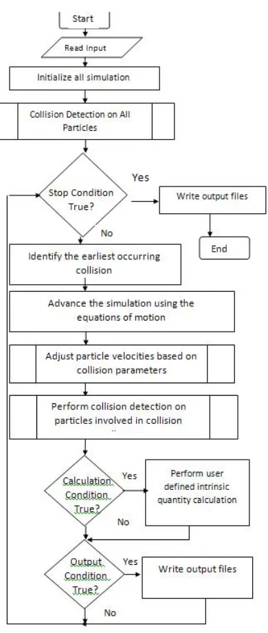
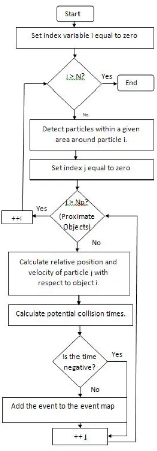
Figure 2.1 A particle on a collision path with two boundaries (solid lines) at the intersection of the boundary (the point). The dashed lines show the extension of the boundaries where collisions will be detected, but rejected on the basis of a non-physicalc value. . . 23 Figure 2.2 A diagram showing the overall flow of the simulation. . . 28 Figure 2.3 A diagram showing the collision detection algorithm. Note that the
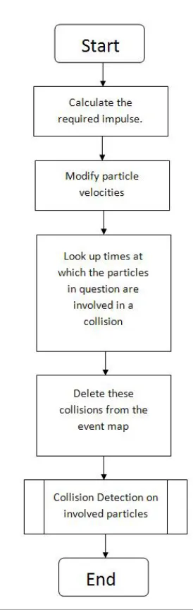
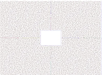
number of loops (i.e., the maximum of the i index variable) depends on the number of proximate objects (particles, points and boundaries) in the given area around the particle . . . 29 Figure 2.4 A diagram showing the collision response algorithm. . . 30 Figure 2.5 A typical starting arrangement for an experimental simulation. Note
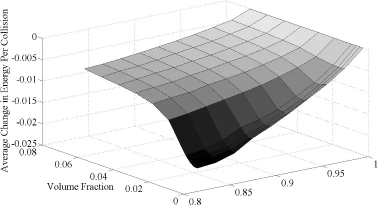
that the apparent overlap of particles is a visualization artifact and does not represent the actual proximity of particles . . . 33 Figure 2.6 The energy change per collision over a range of volume fractions and
coefficients of restitution. . . 34 Figure 2.7 The total energy change over a range of volume fractions and coefficients
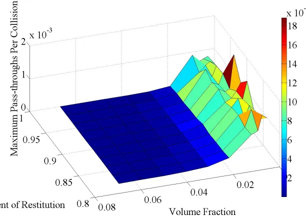
of restitution. . . 35 Figure 2.8 Pass-throughs per collision over a range of volume fractions and
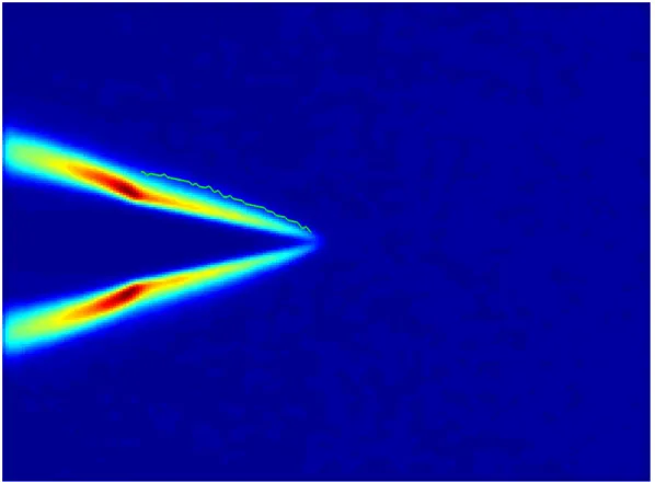
coeffi-cients of restitution . . . 37 Figure 2.9 A sample wedge input initialization file. . . 38 Figure 2.10 A sample wedge output file. The shade of black in the plot indicates
the cumulative count of the number of particles within a given radius of each of the 40,000 lattice points in the simulation with lighter shades representing higher concentrations of particles. Note that the granular material was given an average supersonic velocity downward. The white area of the graph represents a high concentration of particles, and denotes the location of an oblique shock wave in this system. . . 39 Figure 2.11 The average percent difference between a standard simulation final state
and nine others with similar, but not exactly equal, initial states. Quali-tatively, there is no pattern to the percent differences, indicating that the differences are not systematically introduced. . . 39 Figure 2.12 The average percent difference of all ten Criterion 5 computational
ex-periments. Qualitatively, there is no pattern to the percent differences, indicating that the differences are not systematically introduced. . . 40
Figure 3.2 An example of the shock-detection scheme along a given normal to the surface of the wedge shown in Fig.3.1. Both the data along the line and the two lines composing the minimum-error interpolation are shown. The intersection of the two interpolation lines is assumed to be the location of the shock wave. . . 44 Figure 3.3 The variation in oblique shock angle as a function of wedge angle and
average flow velocity. . . 46 Figure 3.4 The variation in oblique shock angle as a function of wedge angle and
average flow velocity. . . 47 Figure 3.5 The variation in oblique shock angle as a function of wedge angle and
coefficient of restitution (e). . . 48 Figure 3.6 The variation in oblique shock angle as a function of wedge angle and
granular temperature. . . 49 Figure 3.7 The variation in oblique shock angle as a function of wedge angle and
initial volume fraction. . . 50 Figure 3.8 An example of a bow shock resulting from supersonic granular flow past
a disc. The estimated shock position shown by the shock detection algo-rithm is shown. . . 51 Figure 3.9 The variation in standoff distance as a function of disc radius and
up-stream average velocity. . . 51 Figure 3.10 The variation in standoff distance as a function of disc radius and
coef-ficient of restitution. . . 52 Figure 3.11 The variation in standoff distance as a function of disc radius and
up-stream granular temperature. . . 53 Figure 3.12 The variation in standoff distance as a function of disc radius and
coef-ficient of restitution. . . 53
Figure 4.1 Time-averaged volume fraction resulting from granular flow over a wedge 56 Figure 4.2 Time-averaged volume fraction resulting from granular flow over a disc . 57 Figure 4.3 Time-averaged volume fraction resulting from granular flow over the
Apollo command module . . . 57 Figure 4.4 Wedge output data showing a sample line along which 1-D data is taken
to identify flow field gradients. This image is color coded by volume fraction. 58 Figure 4.5 The 1-D slice of flow field data taken along the normal line. The optimal
two line fit is shown as well as the estimation of where along this particular normal line the shock wave occurs. . . 59 Figure 4.6 Wedge output data showing the estimated shock wave location on the
upper surface of the wedge. The color in this image represents velocity in the vertical direction, which experiences a higher gradient than volume fraction and thus a better shock wave estimate. . . 59 Figure 4.7 An example of a CFD-ready grid simulating the flow over a wedge. Note
that the grid is clustered relatively tightly around the predicted shock wave location. . . 60 Figure 4.8 An example of the CFD output simulating flow over the wedge shown in
Figure 4.9 The effect of varying Mach number on shock wave angle for granular flows. Granular shock wave positions are generally less sensitive to average
velocity (or Mach number) than those in ideal fluid flows. . . 62
Figure 4.10 Geometric Definitions ofθ and β . . . 62
Figure 4.11 The sensitivity of the granular shock wave angle β to the coefficient of restitution (e) modeling particle interactions. . . 62
Figure 4.12 An analogous granular fluid system constructed to approximate the shock behavior of air. . . 63
Figure 4.13 Granular simulation output: Mach = 3,θ= 10o . . . 64
Figure 4.14 Granular simulation output: Mach = 4,θ= 15o . . . 65
Figure 4.15 Granular simulation output: Mach = 5,θ= 20o . . . 65
Figure 4.16 Grid generation output: Mach = 3,θ= 10o . . . 66
Figure 4.17 Grid generation output: Mach = 4,θ= 15o . . . 66
Figure 4.18 Grid generation output: Mach = 5,θ= 20o . . . 67
Figure 4.19 CFD Mach field results from the efficient grid . . . 68
Chapter 1
Introduction and Review of
Literature
Granular materials can be defined as collections of discrete particles which interact with each
other. Common examples include piles of sand or gravel, silos containing grain, and industrial
powders. The classification of granular materials includes materials that nearly everyone en-counters and interacts with on a daily basis. However, investigating and modeling the behavior
of granular materials are still vibrant areas of of basic science and engineering.
In the remainder of this chapter, I will review the literature pertinent to this dissertation.
I will discuss the history of the study of granular materials and highlight some seminal work
in this vast and diverse field. I will then discuss in more detail the recent work in the study of shock waves in granular materials, and, finally, I will discuss a subset of grid generation
and Computational Fluid Dynamics (CFD) literature that applies to the remainder of the
dissertation.
In Chapter 2, I will discuss the design and implementation of an event-driven hard-sphere
simulator. Such a simulation program was critical to the completion of this dissertation and is
the software with which all of the results presented herein were generated. The simulation was completed in C++ using data structures and algorithms provided in the Standard Template
Library (STL). The use of open-source two-dimensional space discretization algorithms and
efficient pseudo-random number generators was also used.
Chapter 3 will detail the use of the above-mentioned event-driven simulation to examine
the interaction between granular gases of various flow velocities over obstacles. As simulated
granular flows impinge on obstacles, shock waves may be present in accordance with the theory discussed in this literature review and in subsequent chapters.
A novel use of the data gained by simulating supersonic granular flow over an obstacle will
granular flows over a given obstacle is the location of the shock wave in the granular flow.
The shock wave location can serve as an approximation of the location at which a shock wave would occur in analogous fluid flow. Given that most fluid flow simulations use finite element
or finite volume methods to converge to a solution quickly, the location of any shock waves
in the system; i.e., the location at which the fluid properties rapidly change, would be useful to know. As will be seen in Chapter 4, the knowledge of shock wave location can lead to the
creation of better spatial grids on which the solution is calculated using finite element or finite
volume solvers. The results obtained from using these grids in conjunction with a finite volume solver will be shown. Chapter 5 will describe some future directions for the research and results
described in this dissertation.
1.1
Granular Materials In General
Granular materials are ubiquitous in the natural and man-made world. As stated in the
intro-duction, a granular material is simply a discrete collection of particles which interact with each other through contact forces. The study of granular materials has been of practical importance
throughout history to those who have worked with sand, sugar, salt, grain, or, in later years,
industrial powders, pharmaceuticals, or any other large collections of discrete particles. The first recorded observation and study of granular dynamics is Faraday’s observation of granular
conduction cells in the early 19th century, and the scientific study of the behavior of granular
materials has been a topic of intense study for this century and the majority of the last[21]. There are many different reasons to study granular flow. Of primary interest to those in the
applied sciences is the fact that granular materials are so common in both industrial and natural
processes.[34] The literature contains thousands of references to the study of granular materials in specific processes. Examples of popular contexts in which granular materials are studied
include the transport of materials through hoppers or ducts, the description of chemical reactor
beds, the dynamics of avalanches, and the dynamics of soils.[60, 32, 53, 31, 46] The plethora of applications in which the dynamics of granular materials figures prominently has necessitated
investigations into the physical and mathematical nature of granular materials; Over the past
half-century, such investigations have yielded new tools and techniques for describing granular systems and predicting their behavior.
The general description of granular materials in the literature tends to break down along
two types of granular behavior: static granular systems and dynamic granular systems. Re-search into static granular systems is primarily concerned with the structure and stability of
the static arrangement of particles comprising the system. Studying static granular systems gives researchers an insight into why such collections of particles remain in a static, stable
materials. An important figure of merit describing the structure of a static granular system is
the stress distribution in the granular system.[8, 40, 30, 41] Granular stability, or the tendency of a static granular system to remain in a static state, has been related to the angle formed by
a granular pile when it comes to rest.[4] The literature also contains many studies regarding the
precarious nature of granular stability and the transition from a stable, static granular system to a moving granular system; much of this research concerns avalanche dynamics.[19, 38]
Dynamic granular systems, systems whose constituents move with respect to time, have
also garnered much attention from researchers. Rericha details popular types of moving gran-ular systems under experimental and computational study.[50] Moving grangran-ular systems are of
interest to researchers primarily because many applications of granular materials involve their
motion. Furthermore, from a basic research standpoint, moving granular systems are of interest because the fundamental behavior of granular systems can depend on the nature of the motion
of the system. Accurate modeling and prediction of granular material behavior, therefore,
de-pends on detailed knowledge of the behavior of the system both at rest and in motion. Dynamic granular systems will be the focus of this dissertation.
1.2
Shock Waves in Granular Materials
The general definition of a shock wave from fluid dynamics is a spatially small region of flow
across which the fluid properties undergo a sudden change.[7] This definition also applies to
granular flows. Because much of the terminology and descriptive techniques for granular systems are borrowed from the world of fluid dynamics, shock waves in granular systems can best be
understood in the light of analogies to fluid flows. In order to draw analogies between fluid
flows and granular flows, it becomes necessary to be able to describe the conditions under which granular substances exhibit fluid-like properties. The question of classification of granular
materials by state is one that has been studied at great length. As Jaeger, Nagel, and Behringer
discuss, such a classification can be difficult to make.[35, 34] In general, the dynamics of a granular system, and thus the state of a granular system, depend on many factors.
One factor that can be used for state determination is a bulk measurement of the kinetic
energy of components of the granular system. One important bulk measure of kinetic energy is the “granular temperature” of a system.[33] The existence of an appropriate definition of
granular temperature is a topic which has been debated by the granular materials community
for some time, but it is most often defined as the statistical variance of the velocity of the grains in the system. Note that the granular temperature has nothing to do with the actual
thermodynamic temperature of the constituent grains; since the grains are macroscopic, the dynamics of the system is independent of thermodynamic temperature.[28] In general, systems
solid granular behavior; this fact is demonstrated both theoretically and experimentally by
Zhang and Campbell who investigated the dynamics of granular systems at the interface between solid-like and fluid-like granular flow. [63]
In the study of shock waves in granular materials, it is typically the fluid-like phase that
is of most interest to researchers; therefore, to study shocks in granular flow, it is necessary to understand how granular materials come to be in a fluid-like state. The study of the fluidization
of granular materials and the dynamics of fluidized granular materials occupies a large place
in the granular material literature. In general, fluidization of granular materials occurs when the material experiences a small amount of stress[17]; such a condition can occur when the
granular temperature of the material is raised to a sufficient level. There are two main methods
of raising granular temperature: imparting either translational or vibrational motion to the granular material. Translational motion might arise by the transport of granular materials
through industrial devices such as hoppers, channels, or conveyors while vibrational motion is
usually imparted to a granular material through the use of special equipment designed to apply a given force or displacement profile to a material container. Note that the rise in granular
temperature through translation is usually a side-effect of the bulk motion of the material while
the rise in granular temperature due to vibration is usually the intended effect.
Granular fluids have many aspects in common with traditional fluids. Granular analogs
ex-ist for many of the traditional bulk thermodynamic quantities typically used to describe fluids. Researchers have presented formulations for granular temperature, granular pressure, granular
density (also called volume fraction), and other quantities. Many of the same interesting
phe-nomena observed in traditional fluids are also observed in granular fluids; one such phenomenon is the existence of a “speed of sound” associated with granular fluids. This characteristic speed
of a granular fluid is the maximum speed at which information can propagate through the fluid.
At a fundamental level, the speed of sound is related to the average velocity of the fluid con-stituents and the mean free path of the fluid. While information through a granular fluid has
a speed limit, the velocity of disturbances through a granular fluid has no corresponding speed
limit. As with traditional fluids, the fact that disturbances can move through a granular fluid faster than information can propagate through the fluid leads to the fact that shock waves can
be present in the granular fluid. As discussed at the beginning of this section, shock waves are
regions in which the fluid properties change a great deal in a relatively small spatial distance. The existence of shock waves in granular materials has been a strong thread in granular
ma-terials research for decades. Savage, et. al., studied the deformation of rapidly moving groups
of granular materials both analytically and computationally in the early 1980s and made use of simplified granular models studied as early as the 1960.[36, 54] The general mechanics of
granu-lar materials and specifically the propagation of waves through fluidized granugranu-lar materials was
the past decade, researchers have applied the growing memory and processing capacity of
com-puters along with new experimental methods to further research shock phenomena in granular materials. Computational and experimental studies have been undertaken on shock waves in
granular materials in containers which vibrate parallel to the acceleration of gravity.[14, 43, 44]
Interesting pattern formations in oscillated granular fluid beds have also been observed and characterized.[13] Rericha, et. al., studied the flow of granular materials over a two dimensional
wedge and observed the resulting shock waves.[51] In 2004, Rericha produced a thesis which
elucidates in great detail the theory of shocks in granular media, provides a number of exper-imental and computational examples and observations, and provides a wealth of resources for
those wishing to understand granular shock waves.[50] Wassgren, et al, observed and modeled
the flow of granular gas around a spherical particle and noted the presence of a bow shock wave showing the analogous shock wave behavior between real gases and granular gases.[61]
Bharad-waj, Wassgren, and Zenit calculated the drag force on an immersed cylinder[11] and Gray, Tai,
and Noelle experimentally determined surface pressures (in effect, drag) for immersed tetra-hedrons in three dimensional supersonic granular flow.[27] Soleymani, et al, simulated shocks
occurring over a wedge in three-dimensional duct flow.
1.3
Modeling Techniques for Granular Materials
Granular materials themselves are all around the natural and man-made world and it is likely
that most people have interacted with granular materials at some point. However, there is
still much research being performed on the nature of granular materials and their dynamics, and accurate models and predictions of macroscopic granular material behavior are difficult
to come by; there is still much to be learned about granular materials. The dichotomy of a
ubiquitous but mysterious material is an interesting one, and one that drives basic research. Much of the basic research into granular materials has been centered around finding accurate
models to describe the dynamic behavior of granular materials under different regimes. The main goal of models of granular materials is to solve the Boltzmann equation for materials of a
given description.[23] In general, there are two methods that are used to attempt to solve the
Boltzmann equation: theoretical derivation of partial differential transport equations and their corresponding numerical solutions, and numerical solutions obtained by directly simulating
colliding particles. These two methods will be referred to as the hydrodynamic approach and
the molecular dynamics approach.
1.3.1 The Hydrodynamic Approach
dynamics. In particular, the equations of motion are formulated from a continuum viewpoint
and the goal of such equations is to describe the time evolution of changes in bulk quantities. Many of the bulk quantities determined using the hydrodynamic approach are analogous to
thermodynamic quantities. One of the advantages of the hydrodynamic approach is that,
because the granular system under study is thought of as a continuum rather than a set of discrete particles, the computational cost of the approach is, in general, independent of the
number of particles being modeled. Furthermore, because the hydrodynamic approach directly
solves for bulk continuum properties, the results of hydrodynamic computations are in forms familiar and meaningful to scientists; i.e., the hydrodynamic approach results in expressions for
bulk quantities like density, temperature, pressure, partition functions, etc. The hydrodynamic
approach has disadvantages as well. The primary disadvantage to the hydrodynamic approach is that the proper form of the hydrodynamic equations is unknown at this time.
Much of the research into granular materials performed in the past 50 years has been focused
on determining the proper form of continuum equations which describe granular flow.[26] The literature is incredibly dense with substantially different continuum models of granular motion
and a comprehensive review of such literature is out of the scope of this document. However,
the literature seems to suggest that there are two primary reasons for the difficulty to coming to a consensus on the structure of these equations: the fact that most granular systems are
dissipative systems and the lack of a sufficient constitutive law of granular motion[37, 15]. In the practical world, the flow of granular materials is dominated by frictional and impact forces.
It certainly does not help the cause of those who wish to model granular systems that neither
friction or contact forces are, at their most basic levels, very well understood. In practice, most researchers use approximations of the effects of these forces, such as a linear friction model and
a coefficient of restitution model of impacts. Both the validity of these models and the overall
impact of dissipative forces on the structure of the equations describing granular flow are the topics of a wealth of research. Effects such as granular collapse lead to the non-equilibrium
nature and increased complexity of dissipative granular flows. Coupled with the fact that
different flow regimes warrant different constitutive laws, the modeling of granular materials as a continuum presents many difficulties for researchers.
1.3.2 The Discrete Approach
The second approach to modeling granular flow is to directly determine the trajectories for each
of the constituent particles in the granular system. Because this type of technique is used in the world of chemistry to determine the motions and actions of molecules, it is referred to as the
molecular dynamics techniques are distinct from Monte Carlo simulations and typical hard
sphere models in that the trajectories of the particles composing the material are deterministic rather than stochastic and molecular dynamics models tend to employ particles that are neither
hard nor necessarily spherical.[47, 48] One advantage to molecular dynamics simulations and
models of granular flow is that it provides a solid physical basis for the motion of the constituents of granular media; i.e., the motion of the simulated material is as accurate as the calculations of
the forces on the material. The molecular dynamics approach also compartmentalizes aspects
of the calculations of forces, and therefore does not require extensive derivations resulting from the change of a particular force model.
The drawbacks of the molecular dynamics approach are largely related to computational
efficiency. Because granular constituents interact with each other only through contact, the location of the constituents in space must be known at all points during a molecular dynamics
simulation. Efficiently determining the proximity of moving points in space is a subject of
ongoing research in the computer science field and often requires the use of relatively exotic data structures and algorithms such as KD-Trees or kinetic KD-Trees.[39, 9, 3] In general, however,
the simplest molecular dynamics algorithms scale in computational cost with the square of the
number of particles present in the simulation. However, there is often strong motivation to have a large number of particles in a molecular dynamics simulation. The number of particles
needed to achieve a desired result may be set by the nature of the system being studied, e.g., to obtain a given density of particles of a given size, the number of particles is a constant.
For many systems, a higher number of particles also gives either a larger data sampling set, a
longer run time, or finer resolution in the final quantities. Another drawback of the molecular dynamics approach is that the final output of a molecular dynamics simulation takes the form of
a system state (positions, velocities, etc) of particles as a function of time. In order to translate
the system state into meaningful data, some measure of processing is necessary. The post-processing step can take place in parallel with a molecular dynamics simulation (e.g., at the
end of each step forward in time) but extra computational time is still required to translate
the system state into granular temperatures, volume fractions (densities), pressures, or other variables. Depending on the nature of the quantities to be calculated, this extra step may
introduce a nontrivial level of computational expense.
1.4
Granular Analogs for Gases
The primary goal of this dissertation is to use granular systems as a model for gas flow,
specif-ically to identify the regions in which shock waves may occur in gas flow. There exists links between granular flow and models of fluid flow. Many models of granular flow idealize the
for both hydrodynamic and discrete models of granular flow. Such models bear a strong
re-semblance to sphere and disk models of gas flow; sphere and disk gas models are commonly referred to as kinetic models, gaskinetic models, or physical gas models. For simplicity, from
this point forward both the hard sphere model and the hard disk model will be referred to as
hard sphere models, even though in implementation, they are different. Such models have been used to investigate the theoretical nature of real gas models and to simulate gas flows under
certain regimes.[52, 45] The main difference between typical granular models and hard sphere
gas models is the fact that granular models account for dissipative effects; granular collisions lose energy both through non-unity coefficients of restitution and through frictional effects.
The effect of energy loss (commonly referred to as “cooling” since the net effect is to lower
granular temperature) is a topic of ongoing research, but the fact that energy is not constant in a system leads to the lack of a steady state for long-running granular flows and interesting
dynamical phenomena such as inelastic collapse.[42, 59] Since gas flows are typically studied
at equilibrium and conserve energy, the utility of studying granular systems to shed light on properties of real gas systems can be debated. However, the gap between granular systems and
real gases can be bridged by mathematical techniques such as Enskog’s perturbation solution
to the Boltzmann equation and the study of driven granular flows, in which a balance between dissipative granular cooling and granular heating can be achieved.[18, 16]
When perusing the gaskinetics literature, it is interesting to note that the goal of a large portion of the research is to take ideas which make sense in the discrete case and cast them
into a continuum description of a gas; much as granular fluid researchers attempt to cast
granular flow problems into hydrodynamic continuum equations. From a historical perspective, the desire to work in terms of a continuum is understandable since computational models of
systems having many constituents have historically been intractable. Furthermore, statistical
mechanics provides many reliable bridges between discrete particle behavior and continuum behavior. The desire to apply well-studied statistical mechanics tools to both granular and
gaskinetics systems has driven research in both areas; the identification of primitive statistical
mechanics quantities, such the velocity distribution and radial density function of a collection of particles, continues to drive research into hard sphere granular and gaskinetic models. However,
with the current increases in computational processor power and memory capacity, it is likely
that much can be learned from examining the states of actual hard sphere gases modeled via molecular dynamics methods; this dissertation will show specific applications of granular gas
1.5
Some Notes on Computational Fluid Dynamics
The field of computational fluid dynamics is extremely rich. Because of the necessity of
un-derstanding fluid flow scientists and engineers since the days of Courant have sought to find better ways to simplify and and compute solutions to the Navier-Stokes equations. The set
of mathematical tools brought to bear on computational fluid dynamics problems is extremely
large and touches many seemingly disjointed areas of mathematics. The ability to compute solutions to the Navier-Stokes equations is central to the design of aircraft of all kind, and as
such there is a large interest in the aerospace community in tools and techniques which aide in
the solution of fluid flow problems. In further chapters, this dissertation will present a novel method of assisting current Navier-Stokes solvers in performing their tasks, especially when
shock waves are involved in the solution.
There are certainly other methods that have been under study for a long time which tackle
the problem of resolving shock waves in fluid flow. These methods include adaptive mesh [10]
and upwind shock capturing schemes [62] among many others[57]. The details of methods used to handle shock waves in fluid dynamics codes are beyond the scope of this dissertation,
and could encompass a career within themselves. However, note that each of the methods
of handling shock waves in fluid flows takes specific advantage of the nature of the partial differential equations which describe fluid flow. The novelty of the method described herein
is that it takes advantage of not only equations different from the Navier-Stokes equations,
but a different physical process altogether to draw an analog to ideal fluid motion. It would be presumptuous to suggest that the method described in this dissertation will supplant the
methods currently used to solve fluid flow problems which include shock waves, but it is possible
Chapter 2
Granular Material State Solver
Algorithm
2.1
Introduction
The first step in studying the behavior of granular systems from a computational standpoint
is to build simulations of the granular systems of interest. There are currently two main paradigms of granular simulations: continuum simulations and discrete simulations. Continuum
simulations treat the granular system as a continuous body and attempt to use conservation
and constitutive laws to model the dynamics of the system. Such models are typically in the form of partial differential equations in spatial coordinates and time. Discrete simulations track
individual particles and their interactions with other particles as the simulation progresses. Bulk
quantities such as temperature, density, and local sonic velocity can be determined at any point in time using the state (position and velocity) of individual particles.
The continuum and discrete simulation paradigms each have their own advantages and
dis-advantages. Discrete simulations suffer an execution time penalty as the number of particles in the system increases while continuum simulations, since they deal mainly in bulk quantities, are
relatively insensitive to the amount of a granular material involved in a simulation. However,
discrete simulations typically only seek to solve either algebraic or ordinary differential equa-tions while continuum simulaequa-tions seek to solve partial differential equaequa-tions; solving PDEs is
generally much more computationally difficult and expensive than solving ODEs and algebraic equations. This document focuses on the development of a discrete granular simulation using
the Standard Template Library (STL) of C++. Using the C++ STL and techniques from
computer game development and computational geometry, an efficient method of simulating low-density granular flows is established. The simulation has been successfully used to model
2.2
Granular System Model
In order to describe the simulation used to solve the granular system, it is necessary to
dis-cuss the discrete model of the granular system. The simplified model of the granular system consists of spherical particles which interact with each other only through contact forces which
occur during collisions. The collision response of the particles is assumed to be fully described
through the use of the coefficient of restitution of the particle. The particles are assumed to be smooth so that frictional forces can be neglected. The lack of frictional forces also negates the
transfer of angular momentum from particle to particle, therefore the state of each particle
con-sists of its position and translational velocity; the angular velocity of each particle is conserved throughout the simulation and therefore not tracked. The model consists of two spatial
dimen-sions (therefore the “spherical” particles are actually disks), although the equations developed generalize to three spatial dimensions. The model also consists of stationary boundaries with
which the particles can interact. The boundaries are modeled as line segments and are used to
form obstacles to the granular flow. While this granular model is simplified and not likely to simulate real-world granular systems, many of the techniques used to simulate this system can
be generalized to handle a variety of different granular models.
2.3
Simulation Algorithm
2.3.1 General Overview
The general simulation algorithm involves three main steps: the detection of the time at which
the earliest collision occurs (t), changing the state of the system to reflect the passage of time
t, and determining the post-collision state of the system. Because the particles do not interact with each other through forces at a distance (e.g. through gravitational, molecular, electrostatic,
or other forces), the trajectories of each particle in the time between collisions is governed only by the state of the particle and any external force acting on the system. In most practical
applications, the external force acting on the system is a either a uniform gravitational force
or is exactly zero; therefore, the trajectories of the particles in the time between collisions is either a straight line (in the case of zero external force) or an algebraically-defined arc (in the
case of a uniform force). In either case, the path of each particle, and therefore the state of the
system in the time between collisions, is known. The simulation will therefore only keep track of changes in the state of the system as a result of collisions; such a simulation is known as an
2.3.2 Collision Detection
The goal of collision detection is to detect both if and when any two particles will collide or,
alternatively, when a particle will collide with a boundary. Consider two particles denoted A
andBwith positions~r and velocities~vexpressed in a given coordinate system with unit vectors ˆi, ˆj as
~
rA=rAxˆi+rAyˆj (2.1)
~
rB=rBxˆi+rByˆj (2.2)
~vA=vAxˆi+vAyˆj (2.3)
~vB=vBxˆi+vByˆj (2.4)
Furthermore, consider a uniform gravitational force given by
~g=−gˆj (2.5)
The path of each particle as a function of timet is therefore is given by
~
rA= (rAx+vAxt) ˆi+
rAy+vAyt− 1 2gt 2 ˆ j (2.6) ~
rB= (rBx+vBxt) ˆi+
rBy+vByt− 1 2gt 2 ˆ j (2.7)
For spherical particles, the collision condition is
|~rA−~rB|=RA+RB (2.8)
where RA and RB are the respective radii of particles A and B. Mathematically, the collision detection problem is to find the time t at which Eq.2.8 is satisfied. Applying Eqs.2.6 and 2.7 to Eq.2.8 yields
(rAx−rBx+ (vAx−vby)t) ˆi+ (rAy−rBy+ (vAy−vBy)t) ˆj
=RA+RB (2.9)
For brevity, the general substitution
XAz −XBz=XABz (2.10)
r
r2
ABx+r2ABy+ (2rABxvABx+ 2rAByvABy)t+
v2
ABx+v2ABy
t2 =R
A+RB (2.11)
Squaring both sides of Eq. 2.11 yields a quadratic equation int which can be solved
t = −(2rABxvABx+ 2rAByvABy) 2
rABx2 +rABy2
±
r
(2rABxvABx+ 2rAByvABy)2−4
r2
ABx+r2ABy vABx2 +v2ABy
2r2
ABx+r2ABy
(2.12)
Which gives the collision time t in terms of the states of the two particles, which are known. Equation 2.12 will give two results and there are four possibilities regarding the values of the results: both results are imaginary, both results are positive and real, one result is a real
negative number and one result is a real positive number, and both results are negative. In the case of two positive results, a collision will occur and the collision condition will be met at the
smaller of the two values. Note that mathematically, a collision will also occur at the greater
t value, but the velocities of the particles will be modified as a response to the first collision, thus negating the possibility of the second collision. In the case of two negative results, the
particles will only collide if the simulation time is run backwards; this is generally not allowed.
In the case of two imaginary results, this indicate that the paths of the particles will cross, but no parts of the particles will be coincident. In the case of one positive real and one negative
real solution, the collision condition will be met, i.e., the distance between the centers of the
particles will be equal to the sum of the particle radii if the simulation time is allowed to run backwards and if the simulation time is allowed to run forward. The only possibility, therefore,
is that the particles are penetrating each other. The simulation is set up so that this should
not happen and therefore, this condition provides a valuable “sanity check” for the simulation. Along with particle-particle collisions, particles may also collide with stationary boundaries.
In order to detect these collisions, it is first necessary to be able to parameterize a stationary
boundary. It is first assumed that stationary boundaries are represented as line segments. Line segments can be parameterized using their end points by the equation
~r=~rS(1−c) +c~rE; 0≤c≤1 (2.13)
boundary and along a line perpendicular to the boundary. Therefore, the collision condition
can be written
~
rA−~rP =RA~rp⊥ (2.14)
where~rAis a vector locating the center of the particle,~rp is the vector locating the point on the boundary where the collision occurs, and~rp⊥ is a vector of unit length pointing perpendicular
to the boundary. The vector~rp⊥ can be expressed
~rp⊥=
(rEy−rEy) ˆi+ (rEx−rEx) ˆj
q
(rEy−rEy)2+ (rEx−rEx)2
(2.15)
The collision condition Eq. 2.14 can therefore be written
rAx+vAxt+ 1 2axt
2+r
Sx(1−c) +crEx
ˆi (2.16)
+
rAy+vAyt+ 1 2ayt
2+r
Sy(1−c) +crEy
ˆ
j (2.17)
= RA
(rEy−rSy) ˆi+ (rEx−rSx) ˆj
q
(rEy −rSy)2+ (rEx−rSx)2
(2.18)
which can be written as a system of two simultaneous equations as:
rAx+vAxt+ 1 2axt
2+r
Sx(1−c) +crEx=rpx (2.19)
rAy+vAyt+ 1 2ayt
2+r
Sy(1−c) +crEy=rpy (2.20)
where the substitution
rpx=RA
rEy−rSy
q
(rEy−rSy)2+ (rEx−rSx)2
(2.21)
rpy=RA
rEx−rSx
q
(rEy−rSy)2+ (rEx−rSx)2
(2.22)
rASx+crSEx+vAxt+ 1 2axt
2 =r
px (2.23)
rASy+crSEy+vAyt+ 1 2ayt
2 =r
py (2.24)
which uses the same labeling convention introduced by Eq. 2.10. The equations 2.23 and 2.24
represent two simultaneous equations which are quadratic in t but linear in c. Both t (which indicates the time at which the collision occurs) andc(the parameter which indicates where on the boundary the collision occurs) must be determined using Eqs. 2.23 and 2.24. This is done
by solving Eq. 2.24 for c in terms oft and substituting the result into Eq. 2.23. Solving for c
yields
c= rpy−vAyt−
1 2ayt2
rSEy
(2.25)
Substituting Eq. 2.25 into Eq. 2.23 and collecting terms gives
rASx+
rpyrSEx
rSEy
−rpx
+
vAx−
vAyrSEx
rSEy t+ ax 2 −
ayrSEx 2rSEy
t2 = 0 (2.26)
which can be solved fortusing the quadratic equation. The result can then be substituted into Eq. 2.25 to determine the value of the parameter c. It is important to note here that in the absence of an external force acting on the particles, Eqs. 2.19 and 2.20 become simultaneous linear equations intandc. As is the case with particle-particle collisions, the possible values of
tandcindicate whether or not the predicted collision actually occurs. If the calculated value of the parametercis either less than zero or greater than 1, the particle actually “collides” with the extension of the line segment through the plane of the simulation (recall that the simulation is
restricted to two dimensions) and no collision actually occurs. Furthermore, the interpretation
of a negative collision time t is that either the collision occurs only if the simulation time runs backwards or the collision occurs on the side of the boundary pointing away from the 90o
rotation of the vector ~rE −~rS. This indicates that the choice of the “starting” and “ending” points of the line segment making up a given boundary orients the boundary. In practice, this is not necessarily bad since boundaries are used to construct solid regions in the simulation
plane; i.e. regions with an “inside” and regions with an “outside”. For instance, boundaries
can be used to make a triangular cone shape in the simulation plane in order to study the shock waves generated by supersonic flow of a granular gas over the cone. Likewise, thermodynamic
simulations can be carried out in which the granular gas is confined within a certain area of the
such that acceptable collisions (i.e., collisions on the outside of the cone or the inside of the
box) result in positive collision times and negative collision times can be discarded.
It is convenient at this point to introduce a third kind of collision. As stated before,
boundaries can be used to divide the simulation plane into different areas. The intersections of
boundaries are called “points”. It is useful to calculate the time at which particles will collide with points. This is done to handle the special case where a collision between a particle and a
boundary occurs at either the start point~rS or end point of a boundary~rE of a boundary. The particle-boundary collision condition described above will detect collisions on the extension of a line segment through the simulation plane and rejects collisions occurring where c is either greater than 1 or less than 0. However, in certain orientations, a particle colliding only with
one of the ending points of a boundary will go undetected, leading to undesired and unphysical behavior in the simulation. Point-particle collision times can be calculated by assuming that
the point is a particle with zero radius and applying the same equations and conditions as
previously described for determining particle-particle collision times.
2.3.3 Collision Response
As with collision detection, collision response must be handled for three different cases:
particle-particle collision response, particle-particle-boundary collision response, and particle-particle-point collision re-sponse. The derivations used elaborate on work done in the computer game development
industry.[29]. By assumption, the result of particle-particle collisions is an impulsive response
which instantaneously changes the velocity of both of the particles involved in the collision. The strength of the response is a function of the mass of the particles, their relative velocity
along a line connecting the centers of mass, and the coefficient of restitution of the collision.
Therefore, there are two steps in determining the collision response of a particle in two dimen-sions: determining the plane of impact of the particle and determining the magnitude of the
impulse imparted to the particles.
Determining the plane of impact for a particle-particle collision is equivalent to determining the vector location of the center of mass of one particle with respect to the other particle.
Given two spherical particles near the moment of impact whose center of mass locations are
determined by ~rA and ~rB, and therefore a coordinate system with the unit vectors ˆn and ˆt where
ˆ
n= ~rA−~rB |~rA−~rB|
can be defined. Assuming that the system is frictionless, there can be no force transfered in
the ˆt direction at the moment of impact. Therefore, the entire impulse will be directed in the ˆ
n direction. The magnitude of the impulse can be determined by applying the principle of conservation of momentum in the ˆndirection. Defining
~vX ·nˆ=vXn (2.29)
the conservation of momentum in the ˆn direction can be written
mavAn+mbvBn=mav 0
An+mbv 0
Bn (2.30)
where variables with a prime (’) superscript indicate post-collision quantities.
Two intermediary definitions need to be made in order to determine the strength of the impulse. First, the coefficient of restitution of the collision is a measure of how much energy is
lost during a collision. The coefficient of restitution is defined
e= v 0 An−v
0 Bn
vAn−vBn
(2.31)
or
e(vAn−vBn) =v 0 An−v
0
Bn (2.32)
The strength of the impulse (j) is defined such that
v0An = vAn+
j ma
(2.33)
vBn0 = vBn−
j mB
(2.34)
To derive an expression forj, begin with the statement of conservation of momentum in the ˆn
direction (Eq. 2.30). Applying the definition ofe(Eq. 2.31), v0Bn can be eliminated:
evAn+v 0
An = evBn+v 0
Bn (2.35)
v0Bn = v0An−e(vBn−vAn) (2.36)
Equation 2.30 can then be written
mavAn+mbvBn =mav 0
An+mb
v0An−e(vBn−vAn)
(2.37)
vAn0 = mavAn+mbvBn+mBe(vBn−vAn)
mA+mB
(2.38)
Equation 2.38 can be substituted into Eq. 2.33 in order to solve for an expression for the impulse
strength (j).
mavAn+mbvBn+mBe(vBn−vAn)
mA+mB
− j
mA
= vAn (2.39)
mA
mA+mB
(mAvAn+mBvBn+mBe(vBn−vAn)−mAvAn−mBvAn) = j (2.40)
mAmB(1 +e)
mA+mB
(vBn−vAn) = j (2.41)
1 +e
1
mA +
1
mB
(vBn−vAn) = j (2.42)
Substituting Eq. 2.42 into Eqs. 2.33 and 2.34 reveals expressions for the post-collision velocities
vAn0 and vBn0 in terms of the pre-collision velocity of the two colliding particles, the masses of the particles, and the coefficient of restitution of the collision.
vAn0 = vAn+ 1 +e
1 + mA mB
(vBn−vAn) (2.43)
v0Bn = vBn+ 1 +e
1 +mB mA
(vAn−vBn) (2.44)
In the simulation of a multi-particle system, the collisions between two particles and the collisions between particles and objects in the environment must be described. The collision
between a particle and a boundary can be described using the same equations derived above
with some additional assumptions made.
The first assumption is that there is no impulse transmitted to the particle along the
di-rection parallel to the boundary. This is the same “frictionless” assumption that was made for
particle-particle interactions. The second assumption is that the normal direction of the colli-sion is (the direction of ˆn) is normal to the boundary. Using these two assumptions, Eqs. 2.43 and 2.44 describes the post-collision velocities of spherical particles and linear boundaries in
1 +e
1
mA +
1
mB
(vBn−vAn) = j (2.45)
1 +e
1
mA
(vBn−vAn) = j (2.46)
these boundaries are assumed to be of constant velocity in the system; usually, this velocity is
zero. Therefore, in the case that a particle impacts a stationary boundary, the final velocity is given by
v0An = vAn+ (1 +e) (vBn−vAn) (2.47)
v0At = vAt (2.48)
where the normal vector ˆn is perpendicular to the boundary and the tangential vector ˆt is parallel to the boundary.
The final type of interaction that must be described is the particle-point interaction. As with collision detection, the point collision response uses the same equations as
particle-particle collision response with the point modeled as a infinitely massive particle-particle of zero radius.
Therefore, the post-collision velocity of a particle colliding with a point is given by
v0An = vAn+ (1 +e) (vBn−vAn) (2.49)
v0At = vAt (2.50)
where the normal vector ˆndirected along the line connecting the center of mass of particle A
and the point; the vector ˆtis directed perpendicular to this line.
2.3.4 Simulation Advancement
After collision detection and collision handling, the third major component of an event-driven algorithm is updating the state of each particle in the system to reflect a given passage of time
~
rA=~rAo+~vAo+ 1 2~at
2 (2.51)
~
vA=~vAo+~at (2.52)
where X~A is the vector quantity (either position or velocity) of a particle A after a period of timet andX~Ao is the initial vector quantity prior to the advancement of the system.
At this point it is important to note that simple equations can be used to describe the path and velocity of the particles in the system because, by assumption, the particles in the system
are acted on by a single constant external force. Therefore, the solutions to the differential
equations of motion are known to be Eq. 2.51 and Eq. 2.52. In the case that the algebraic form of the solutions of the differential equations of motion are not known, the simulation
advancement step would involve numerically approximating the solutions to the equations of
motion. The study of molecular dynamics is one which often uses simulations reminiscent of granular simulations to model the motion of molecules. In molecular dynamics simulations,
potentials of various forms are used to model the interactions between molecules and thus the
simulations must be written to accommodate numerical solutions in the advancement step. The introduction of numerical solutions to the equations of motion also removes the event-driven
character of the simulation since it is often necessary to consider times steps much smaller
than the minimum time step between collisions to determine the path of the particles between collisions. Therefore, the constant force assumption (and mathematically, the assumption of
any force for which the solutions of the equations of motion can be solved algebraically) is a simplifying assumption.
2.4
Standard Template Library Implementation
Most modern implementations of C++ provide access to basic datatypes and algorithms nec-essary to successfully use the language to efficiently solve scientific and engineering problems.
However, there are many data structures and algorithms, particularly those utilizing dynamic
memory management, that do not have implementations in standard C++. Some examples of data structures that are not part of basic C++ implementations include linked lists and
trees; both of which are useful in the modeling and simulation community. The Standard
Template Library was developed to provide an “extended”, standardized set of data structures and algorithms that meet the needs of users interested in implementing dynamically allocated
data structures. More specifically, the Standard Template Library (STL) provides template
structures. This section will detail the use of the vector and map STL containers to implement
an event-driven granular gas simulation.
In developing the granular gas simulation, several options were available. The choice was
made to write the simulation in a compiled language rather than an interpreted language in
order to decrease the run time of the simulation. The two most common choices for scientific programming in compiled languages are C++ and FORTRAN. The choice of C++ rather than
FORTRAN was made for several reasons, the first of which was that the people involved in
this project are simply more experienced in C++ than in FORTRAN. However, there have been several developments in recent years that make C++ an attractive choice for modeling
and simulation; one such development is the publication of libraries such as CGAL[2] and
Boost[1] which offer complex, speedy algorithms capable of quickly performing a wide array of calculations. The continued proliferation of object oriented computer resources also makes the
choice of C++ a more attractive choice for developing new modeling and simulation tools. The
goal of this project was to create a simulation which was fast in execution and still relatively simple to implement and debug; therefore, the simulation described in this document avoids
more complex libraries such as CGAL and Boost and uses the simpler, more standardized
Standard Template Library. However, there is potential utility in using more complex source code in future projects; this will most likely be a focus of future work.
The simulation described below seeks to efficiently determine the state of a two-dimensional system comprised of a given number of interacting spherical particles and linear boundaries.
In order to investigate several different simulation algorithms quickly, the relatively simple
structures provided by the C++ Standard Template Library were used. The following sections describe the simulation data types and the algorithms and equations used to simulate the
behavior of the granular system.
2.4.1 Model Data Types
In order to describe the implementation of the event-driven algorithm detailed above, there are some general data types and functions which are convenient to define. Consider a datatypevect
as an STL vector container of user-defined size containing double precision real numbers. As
the name suggests, a vect will be used to represent mathematical vector quantities and to build up dynamically allocated arrays (STL vectors containing vects). We also define vector addition,
subtraction, dot and cross products as functions taking vects as arguments and returning vects
either vects or double precision numbers where appropriate.
We define two C++ structs (C++ aggregate data types) particle and particletype to store
the particle) and an integer type number indicating the particletype describing the particle.
The particletype struct contains the information necessary to parameterize the particle and its interactions with other particles and boundaries; this data includes the particle mass, the
particle radius, and the coefficient of restitution associated with particle and
particle-boundary collisions. If there is a diversity of particle masses, radii, or coefficients of restitution present in the simulation, there is one particletype entry for each unique combination of particle
radius, mass, and coefficient of restitution. In practice, there may be tens of thousands of
particles described in a simulation and most of the particles are of identical types; the separation of the particle state and particle type allow many different particles to be associated with a
single type, thus reducing the size of input and output files and the memory requirements of
the simulation.
We also define a struct boundary to hold information relating to the linear boundaries
present in the simulation. The system boundaries are regions which have a defined interaction
with particles and, as line segments, they may be completely described by their starting and ending points using Eq. 2.53.
~
rb=~rs+c~re
0≤c≤1 (2.53)
where~rb is the set of points composing the boundary,~rs is the starting point of the boundary and~reis the ending point of the boundary. The geometric information regarding the boundary starting point, the boundary ending point, and the vector normal to the boundary are all defined in separate vects within the boundary struct. Therefore, the first two elements of the boundary
struct are two dimensional vectors representing the end point and the beginning point of the
boundary with respect to the global origin. As the normal vector to the boundary is used in the particle-boundary collision detection and collision response algorithms, the normal for each
boundary in the simulation is calculated when the simulation is initialized and stored as a third
vect in the boundary struct.
The third category of physical object we wish to represent consists of the points in the
simulation space; we therefore define the structPoint to hold information about points. Points
occur at the intersections of two boundaries. Points are technically part of boundaries; however, it is convenient to detect particle-point collisions during the simulation. Consider the case in
which a particle is approaching the intersection of two boundaries, as illustrated in Fig. 2.1.
In detecting collisions between particles and boundaries, the simulation uses vector methods to simultaneously solve for the time at which the collision occurs, and the value of the parameter
Figure 2.1: A particle on a collision path with two boundaries (solid lines) at the intersection of the boundary (the point). The dashed lines show the extension of the boundaries where collisions will be detected, but rejected on the basis of a non-physical cvalue.
(i.e., if the collision is with the dotted extension of the boundaries shown in Fig. 2.1). Rather
than monitoring for a collision with a c value of exactly one or zero in order to determine collisions with points, it is more efficient to calculate the locations of the points and to monitor
the system for collisions with points specifically. The strategy of modeling boundary
intersec-tions as points is made more efficient by the fact that points can be modeled as zero-radius particles and the same collision-detection routines can be used for particle-particle collisions
and particle-point collisions.
The fourth struct that we will define is a struct containing the parameters of the simulation itself; we will call this the simulation struct. The simulation struct contains information such
as the location of, names of, and stream pointers to the simulation input and output files,
the overall simulation time and number of simulation iterations, the total number of particles, boundaries, and points, the simulation measurement parameters, and much more information.
The purpose of the simulation struct is to provide a single variable which can be passed by
reference to various simulation functions. Passing the simulation data by reference allows functions to be written assuming that any necessary information is present within the scope
of the function and allows the functions to directly modify the variables contained within the
simulation struct. The model data types are summarized in Table 2.1.
2.4.2 Event Data Types
In order to use the data described above to implement an event-driven simulation, we make
Table 2.1: Model Data Types
Datatype Name Models Contains
Particle Granular particles Position vector (vect),Particle type (int)
Particle type Common particle attributes
radius (double), coefficient of restitution(double), mass (double) Boundary, Stationary boundaries Point Boundary intersections start point (vect), end point (vect),
normal (vect)
Simulation The simulation state
All simulation, event, and calcula-tion data types, IO stream pointers, counters, flags, etc.
implements a user-defined ordering scheme. A standard C++ array, and even dynamically al-located STL vectors, use a zero-starting numbering scheme to label the elements. The elements
of a four element array (or vector) A are accessed using the syntax A[0], A[1], A[2], A[3]. A map however, lets the user define the indexing variable and type. For instance, the elements of a four element map using string indices could be accessed using the syntaxA[f irst],A[second],
A[third],A[f ourth] as long as the map is initialized to accept strings as the index variable type and the ordering of the index variables is defined.
We use an STL map to store information about the detected collisions at each time step in
the system. We will refer to this structure as the event map. The event map key, the variable
which is used to index the map, is the time at which the collision occurs; this is a double precision real number. The index ordering is defined as ascending by collision time. A collision
occurring at timet= 0.473, for example, would be stored ineventmap[0.473] whereeventmap
is the name of the event map object. As the event map is constructed, it is automatically sorted such that the first event map element refers to the earliest occurring collision. The first
element in the event map (representing the earliest-occurring collision) can be automatically
referenced using the STL-definedupper bound()function with an argument of 0.0; this reference will return both the collision data and the time at which the collision occurs.
Each event map element contains an event struct. The event struct contains three
in-teger STL vectors. Recall that the event map is indexed by the simulation time until the predicted collision occurs. In the case that two pairs of objects collide at the same time, the
first vector classifies the collisions occurring at the key time value as either particle-particle,
particle-boundary, or particle-point collisions. The second and third vectors contain integers which identify the index of the particle, boundary, or point involved in the collisions occurring