Integral and differential equations for conformal mapping of bounded multiply connected regions onto a disk with circular slits

(1)

Journal of Fundamental Sciences Vol. 7, No. 1 (2011) 12-18.

ISSN 1823-626X

Journal of Fundamental Sciences

available online at

http://jfs.ibnusina.utm.my

Integral and differential equations for conformal mapping of bounded multiply

connected regions onto a disk with circular slits

Ali H.M. Murid1, Ali W. Kareem Sangawi1 and M.M.S. Nasser2,

1

Ibnu Sina Institute for Fundamental Science Studies, Universiti Teknologi Malaysia, 81310 UTM Skudai Johor, Malaysia.

2

Department of Mathematics, Faculty of Science, Ibb University, P. O. Box 70270, Ibb, Yemen.

Received 25 December 2010, Revised 5 January 2011, Accepted 10 January 2011, Available online 21 Januari 2011.

ABSTRACT

Conformal mapping is a useful tool in science and engineering. On the other hand exact mapping functions are unknown except for some special regions. In this paper we present a new boundary integral equation with classical Neumann kernel associated to fc f , where f is a conformal mapping of bounded multiply connected regions onto a disk with circular slit domain. This boundary integral equation is constructed from a boundary relationship satisfied by a function analytic on a multiply connected region. With fc f known, one can then treat it as a differential equation for computing f . | Conformal mapping | Boundary integral equations | Multiply connected regions | Boundary relationship | Differential equations |

1. INTRODUCTION

Integral equation methods for conformal mapping of

multiply connected regions is currently still a subject of

importance. Nehari [1, p. 334] described the five types of

slit region as important canonical domain regions for

multiply connected regions. They are the parallel slit region,

the circular slit region, the radial slit region, the disk with

concentric circular slits, and the annulus with concentric

circular slits. In general the exact mapping functions are

unknown except for some special regions.

Several methods for numerical approximation for the

conformal mapping of multiply connected regions have

been proposed in [2, 3, 4, 5, 6, 7, 8, 9]. Recently,

reformulations of conformal mappings from the bounded

multiply connected region onto a previous five canonical

slit domains as a Riemann-Hilbert problem are discussed in

Nasser [10]. Murid and Hu [11] formulated an integral

equation method based on the multiply connected Neumann

kernel for conformal mapping of bounded multiply

connected regions onto a disk with circular slit but the

boundary integral equation involved the unknown circular

radii.

In this paper we describe an integral equation method

for computing the conformal mapping of multiply

connected regions onto a disk with circular slits.

Corresponding author at: Ibnu Sina Institute for Fundamental Science Studies, Universiti Teknologi Malaysia, 81310 UTM Skudai Johor,Malaysia. E-mail addresses: [email protected] (Ali H.M. Murid)

This boundary integral equation is constructed from a

boundary relationship satisfied by a function analytic on a

multiply connected region.

The plan of the paper is as follows: After

presentation of some auxiliary material in Section 2, we

derive in Section 3 a boundary integral equation satisfied by

f

c

, where

f

is a conformal mapping of bounded

multiply connected regions onto a disk with circular slit

domain. Section 4 give a numerical implementation for

computing

f

c

f

. In Section 5, we give three examples for

verifying our boundary integral equation that was given in

Section three. Finally, Section 6 presents a short conclusion.

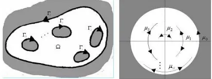
2. NOTATIONS AND AUXILIARY MATERIAL

Let

:

be a bounded multiply connected region of

connectivity

M1

. The boundary

*

consists of

M 1

smooth Jordan curves

*₀,*₁,...,*_M

such that

*₁,...,*_M

lies in the interior of

*₀

, where the outer curve

*₀

has

counterclockwise orientation while the inner curves

M *

*₁,...,

have clockwise orientation. The positive

direction of the contour

* *₀*₁*_M

is usually

that for which

:

is on the left as one traces the boundary

(see Figure 1).

The unit tangent to

*

at

z

is denoted by

z z z

T c c

, and if

f

is analytic function which maps

:

conformally onto a disk with circular slit, then we have the

boundary relationship [11, p. 1126].

(2)

| 13 |

, .

2 2 2 2

2 _*

c c

z

z f

z f z T z f z

f 1

Suppose that k is a complex constant, Qz and H z are complex-valued functions defined on * such that

0

z z

H , Qz z0 and H

z

T z Qz

satisfies the Holder condition on *. Then the interior relationship is defined as follows:

A complex-valued function Pz is said to satisfy the interior relationship if Pz is analytic in : and satisfies the non-homogeneous boundary relationship

_, _*_, _P _z _H _z _z

z G

z Q z T k z

P 2

where Gz is a complex-valued function, analytic in :,

Holder continuous on *, and G z z0 on *.

Figure 1. Mapping of the bounded multiply connected region : of connectivity M1 onto a disk with circular slits.

The following theorem gives an integral equation for an analytic function satisfying the interior relationship (2) [12, p. 45].

Theorem 1:

Let z*, U z and V z be any complex-valued

functions that are defined on *. If the function P z

satisfies the interior relationship, then

, 3

Re

, 2

1

z L z U w G z w

w P s z kU

dw w P w z K PV z P z Q z T

z U z V

R M

j w aj

*

» » ¼ º «

« ¬ ª

» ¼ º «

¬ ª

¦

³

where

,

2 1

, _»

¼ º «

¬ ª

w z

w T z V w Q z w

z U i w z K

S 4

, 5

2 1 2

1

dw w T w Q z w

w H i

PV z T z Q

z H z

LR

³

*

S

and the sum is over all those zeros a₁,a₂,...,a_M of G

that lie inside :. If G has no zeros in :, then the term containing the residue in (3) will not appear.

3. THE BOUNDARY INTEGRAL EQUATION FOR

CONFORMAL MAPPING OF MULTIPLY CONNECTED REGIONS

This section gives an application of Theorem 1 to conformal mapping of multiply connected regions to disk with circular slit domain. Let f z be the mapping function which maps the domain : in the z-plane onto a canonical domain of the disk with circular slit domain in the w-plane. The function f is made uniquely determined by

prescribing that f a 0 and fca !0. Thus the function

f can be written as [10, p. 134]

_z _z_a

_eza hzD_,

f 6

where h is an analytic in : and D is real constant. Taking the derivative of both sides of the equation (6) and dividing both sides by f yields

z z a

h z h

a z z f

z

f _c

c 1

. Then

z z a

h z h

a z z f

z f z

D c

c 1

is analytic in :.

Thus

. 1

a z z D z f

z f

c

7

Note that equation (1) can be written in the following form

. ,

2 2

2

* ¸¸¹ · ¨¨© § c

c

z z f

z f z T z f

z f

8

From equations (7) and (8), and after some arrangement

yields

1 , .

2 2

*

z

a z a z

z T z D z T z

(3)

| 14 | Comparison of equation (2) and equation (9) leads to a choice of P

z Dz , k 1, Q

z T z , Gz 1,

a z a z z T z H

2 1 , U

z T z Q z and V z 1.

Substituting these assignments into (3) leads to an integral equation,

10 . , 2 1 2 2 * » » ¼ º « « ¬ ª *

³

z z L z T dw w D z w w T w T z w z T i PV z D R S

Note thatGz does not have any zeros in :

because Gz is a constant function so the term containing the residue does not appear in (10). Multiply both sides of

(10) by T z and using the fact that T

zT z T z 2 1,

gives

, , 11

2 1 * » ¼ º « ¬ ª *

³

z z L z T dw w T w D z w z T z w z T i PV z D z T R S Where

, . 12

2 1 1 2 1 2 1 2 * » ¼ º « ¬ ª

³

* * z dw a w z w w T i PV z T dw a w z w i PV z T a z z T a z z T z L z T _R S S Since

wa

wz

zaª«¬wzwa»¼º

1 1 1 1

,

and for z*, a: by [4, p. 91]

2 1 1 2 1

³

_* dw z w i

S , 1

1 2 1

³

* dw a w i

S . Thus

w z

w a

dw

z a

i PV

³

_* 2

1 1

2 1

S .

Substituting this result into equation (12) and using the fact that T wdw dw , gives

, . 13

2 1 2 1 *

³

* z dw a w z w w T i PV z T a z z T a z z T z L z T R S Let z f z f z

F c . Then

1 . 14

a z z F z D

From equations (11), (13), and (14) we get

15 . , 2 1 2 1 2 1 * u » ¼ º « ¬ ª

³

* * z a z z T dw a w z w w T i PV z T dw w F w T z w z T z w z T i PV a z z T z F z T S S

Also by using [4, p. 91] and the fact that T w dw dw,

gives

w z

w a

dw

z a

w T i PV

³

* 1 2 1 2 1 S .

Substituting this result into equation (15) yields

. , 2 1 * » ¼ º « ¬ ª

_³

* z a z z T a z z T dw w F w T z w z T z w z T i PV z F z T S

The above integral equation can also be written briefly as

, 1 , , 16

1 *

_³

* z a z z T a z z T dw w F w z N z F where

z T z F z

F1 ,

>

@

° ° ° ¯ °° ° ® * c c cc z * »¼ º «¬ ª . if , Im 2 1 , , , if , Im 1 ,

3 z w

t z t z t z w z w z w z z T w z N S S

(4)

| 15 | uniquely solvable. So we need to modify the integral equation to solve it numerically.

Note that a: and h

z z a

h z

a z z f z f c c 1 so

by using the fundamental theorem [14, p. 164] and the fact

that Tw dw dw, gives

0 2 1 1 1

³

* dw w F

S , 17

By using the same manner we can show that

0 2 1 2 1

³

* dw w F

S , …, 2 0

1 1

³

* M dw w F

S . 18

We can combine the conditions (17) and (18) in the following form . ..., , 2 , 1 , 0 2 1

1 w dw q M

F q

³

* S 19

Thus the integral equation (16) with the condition (19) has a unique solution.

By solving the integral equations (16) and (19) simultaneously for F₁, we can obtain the function Fand hence determine D. With D known, one can then treat (7) as a first order ordinary differential equation for computing

f , as follows

. 1 z f a z z D z f »¼ º «¬ ª

c 20

After finding f we can calculate the radii by taking the modulus for f .

4. NUMERICAL IMPLEMENTATION

In this section we first describe in detail a numerical method for computing the mapping function F₁ for the case of doubly connected region. Using the parameterizations

t

z0 of *0 for t:0dtdE0 and z1t of *1 for

1

0 : dtdE

t the system of integral equations (16) and (19) become

_, _, ₂₁

Im 2 2 1 , , 0 0 0 0 0 1 1 1 1 0 0 0 0 1 0 0 0 1 1 0 * » ¼ º « ¬ ª c ¸ ¹ · ¨ © § c

³

t z a t z t z T i ds s z s z F s z t z N ds s z s z F s z t z N t z F E E S

22 . , Im 2 2 1 , , 1 1 1 1 0 1 1 1 1 1 0 0 0 1 0 1 1 1 1 0 * » ¼ º « ¬ ª c ¸ ¹ · ¨ © § c

³

t z a t z t z T i ds s z s z F s z t z N ds s z s z F s z t z N t z F E E S

Multiply both sides of equations (21) and (22) by z0c t

and z1ct respectively, yields

_, _, ₂₃

Im 2 2 1 , , 0 0 0 0 0 1 0 1 1 1 0 0 0 0 0 1 0 0 0 0 1 0 1 0 * » ¼ º « ¬ ª c c u ¸ ¹ · ¨ © § c c u c c

³

t z a t z t z T t z i ds s z s z F s z t z N t z ds s z s z F s z t z N t z t z F t z E E S

24 , , Im 2 2 1 , , 1 1 1 1 1 1 0 1 1 1 1 1 0 0 0 1 0 1 1 1 1 1 1 0 * » ¼ º « ¬ ª c c u ¸ ¹ · ¨ © § c c u c c

³

t z a t z t z T t z i ds s z s z F s z t z N t z ds s z s z F s z t z N t z t z F t z E E S Defining

₀

,

1 0

0 t zc t F z t

I I₁t z₁ct F₁ z₁t ,

t s

z t N

z

t z s

K₀₀ ₀, ₀ ₀c ₀ , ₀ ,

¸ ¹ · ¨ © § c S 2 1 ,

, ₁ ₀ ₀ ₁

0

01t s z t N z t z s

K ,

t s

z t N

z

t z s

K₁₀ ₁, ₀ ₁c ₁ , ₀ ,

¸ ¹ · ¨ © § c S 2 1 ,

, ₁ ₁ ₁ ₁

1

11t s z t N z t z s

(5)

| 16 |

» ¼ º «

¬ ª

c

a t z

t z T t z i t

0 0 0

0 2 Im

\ ,

» ¼ º «

¬ ª

c

a t z

t z T t z i t

1 1 1

1 2 Im

\ ,

the system of equations (23) and (24) can be briefly written as

25 ,

, ,

0 0

1 1 0 01 0

0 0 0 00 0

1 0

t ds s s t K ds s s t K t

\ I I

I E

_³

E

_³

26 .

, ,

1 0

1 1 1 11 0

0 0 1 10 1

1 0

t ds s s t K ds s s t K t

\ I I

I E

_³

E

_³

Since the functions I and K in the above systems

are periodicE , a reliable procedure for solving equations (25) and (26) numerically is by using the Nystrom's method [15] with the trapezoidal rule. The trapezoidal rule is the most accurate method for integrating periodic functions numerically [16, pp. 134-142]. We choose

S E

E₀ ₁ 2 and n equidistant collocation points ,

1 0 n

i

ti E 1didn on*0 and m equidistant

collocation points t~i ~i1E1 m, di dm ~

1 on*1.

Applying the Nystrom's method with trapezoidal rule to discretize equations (25) and (26), we obtain

27 ,

, ,

0

~ 1 1

~

~ 01 1

1

0 00 0 0

i j m

j j

i n

j

j j i i

t t t t K m t t t K n t

\ I E

I E

I

_¦

28 ,

, ,

~ 1 1 ~

~ 1 ~ ~ 11 1

1

0 ~ 10 0 ~ 1

i m j

j j i n

j

j j i i

t t t t K m t t t K n t

\ I E

I E

I

_¦

Equations (27) and (28) lead to a system of

nm

non-homogeneous linear complex equations in n unknowns

i

t 0

I ,m unknowns I₁ t_i~ . By defining the matrices

j i j

i K t t

n

B E0 ₀₀ , _,

j i j

i K t t

m

C~ E1 ₀₁ , ~ ,

j i j

i _n K t t

D~ E0 ₁₀ ~, , _i _j K t_i t_j m

E~~ E1 ₁₁ ~, ~ ,

i

t 0 i 0

x I , ₁ t~_i

i ~ 1

x I ,

i

i t

b0 \0 , b1i~ \1 ti~ ,

the system of equations (27) and (28) can be written as

nm

by

nm

system of equations

>

I_nnB_nn

@

x_0nC_nmx_1m b₀_n, 29

>

@

x .

x_0n _mm _mm _1m ₁_m

mn I E b

D 30

The result in matrix form for the system of equations (29) and (30) is

, x

x

1 0

1m 0n

¸ ¸ ¸

¹ ·

¨ ¨ ¨

© §

¸ ¸ ¸

¹ ·

¨ ¨ ¨

© §

¸ ¸ ¸

¹ ·

¨ ¨ ¨

© §

m n

mm mm mn

nm nn

nn

b b

E I D

C B

I

31

Defining

, A

¸ ¸ ¸

¹ ·

¨ ¨ ¨

© §

mm mm mn

nm nn

nn

E I D

C B

I

¸ ¸ ¸

¹ ·

¨ ¨ ¨

© §

1m 0n

x x

x and

¸ ¸ ¸

¹ ·

¨ ¨ ¨

© §

m n

b b b

1 0

,

the

nm

by

nm

system can be written briefly as

b

x

A .

5. NUMERICAL EXPERIMENT

For numerical experiments, we have used three test regions based on the examples given in [5, 17, 18]. All the computations are done using MATHEMATICA 7.1 (16 digit machine precision).

The test regions are annulus, circular frame and frame of Limacon. N number of collocation points on each boundary has been chosen. The sub-norm error results between exact values for fc f and their approximations

fc f

n are shown in Tables 1, 2 and 3.

Example 1 Annulus:

(6)

| 17 | Consider a frame of circular annulus A

^

z:~r z 1

`

,

0 , ~ _q _eSW _W_!

r .

^

zt cost isint

`

:

0

* ,

^

zt r~cost sint

`

:

1

* .

The exact mapping function is given by [17]

32 ,

2 0 ,

2 log 2

1

2 log 2

1

4 4

2 SW

V V SW T

V SW T

V

¸ ¹ · ¨

©

§

¸ ¹ · ¨

©

§

i i z i

i i z i e z f

with P e2V and T₄ being the Jacobi Theta-functions. We have chosen W 0.5, ~r eSW and V 0.2. Since

2

0

4SWi

T [17], this implies a e2V P.

Table 1. Error norm (Annulus)

m n

f

n

f f f f

16 1.0 (-02) 32 1.6 (-05) 64 4.6 (-11) 128 1.0 (-14)

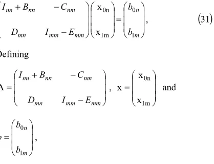
Example 2 Circular Frame:

Figure 2. Circular Frame: with c 0.3,U 0.1.

Consider a pair of Limacon [18]

^

`

, :

0 zt eit *

^

`

, :0 2 , :

1 U d d S

* zt c eit t t

such that the domain bounded by *₀ and *₁is the domain

between a unit circle and a circle center at c with radius U.

Since T₄

SWi 2

0 and r~ q eSW, this implies

S W

r

~ ln

and _V

V

O O

2 2

1

e e

a . We choose a real number V

satisfying 0VSW 2. Then the exact mapping function

is given by

33 , 2 0 ,

2 log

2 1

2 log

2 1

4 4

2 _V SW

V SW T

V

¸ ¹ · ¨

©

§

¸ ¹ · ¨

©

§

i i z p i

i i z p i e z f

where

1

z z z p

O

O _with

2 2

2

12

1 1

1

2

U U

U O

c c c

c

,

2 2

2

12

1 1

1

2 ~

U U

U

c c c

r .

Table 2. Error norm (Circular frame) with c 0.3,U 0.1,V 0.5

m n

f

n

f f f f

8 5.7 (-03) 16 3.3 (-06) 32 1.5 (-12) 64 1.7 (-14)

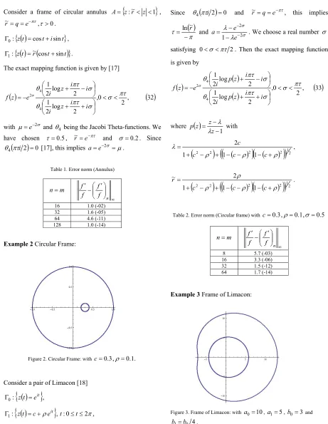
Example 3 Frame of Limacon:

Figure 3. Frame of Limacon: with a₀ 10,a₁ 5,b₀ 3 and

4

0 1 b

b .

(7)

| 18 |

^

`

, 0 , 0 , 2 sin sin 2

cos cos :

0 0 0 0 0

0 0

! !

*

b a

t b t a i t b t a t z

^

`

, 0 , 0 , 2 sin sin 2

cos cos :

1 1 1 1 1

1 1

! !

*

b a

t b t a i t b t a t z

with 10a₀ , 5a₁ , 3b₀ and b₁ b₀ 4 where

S

2 0 : dtd

t . The value of a₀, a₁, b₀ and b₁are chosen so

that b₁ b₀ a₁ a₀and ~r a₁ a₀. Since T₄

SWi 2

0 and

SW

e q r

~ _{, this implies}

S W

1 0

lna a

and

0 2 0 2 0 2 0

4 2

b a a e b

a

V

. We choose a real number V

satisfying 0V SW 2. The exact mapping function is

given by

34 , 2 0 ,

2 log

2 1

2 log

2 1

4 4

2 _V SW

V SW T

V

¸ ¹ · ¨

©

§

¸ ¹ · ¨

©

§

i i z p i

i i z p i e z f

where

P 2V

0 0 2 1

0 2 0

, 2

4

e b

a z b a z

p .

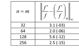
Table 3. Error norm (frame of Limacon) with V 0.1

m

n

f

n

f f f f

32 3.1(03)

64 2.0(06)

128 5.6(12)

256 2.5(15)

6. CONCLUSION

From this study, we have constructed a new boundary integral equation for conformal mapping of regions of connectivity M 1 onto a disk with circular slits. The boundary integral equation for fc f involved the classical Neumann kernel, where f is a conformal mapping of bounded multiply connected regions onto a disk with circular slit domain. The advantage of our method over [11] is that our boundary integral equation does not involve the unknown circular radii. Discretized integral equation leads to a system of linear equations. With fc f known, one can then treat it as a differential equation for computing

f .

ACKNOWLEDGEMENT

This work was supported in part by the Malaysian Ministry of Higher Education (MOHE) through the Research Management Centre (RMC), Universiti Teknologi Malaysia (FRGS Vote 78479). This support is gratefully acknowledged.

REFERENCES

[1] Z. Nehari, Conformal Mapping, Dover Publications, Inc, New York, 1952.

[2] D. Crowdy, and J. Marshall, Computational Methods and Function Theory 6 (2006) 59-76. [3] S.W. Ellacott, Numerische Mathematik 33 (1979) 437-446.

[4] P. Henrici, Applied and Computational Complex Analysis, Vol. 3, John Wiley, New York, 1974. [5] P.K. Kythe, Computational Conformal Mapping, Birkhauser Boston, New Orleans, 1998. [6] A. H. M. Murid and N. A. Mohamed, Int. J. of Pure and Appl. Math. 38(2007), 229-250. [7] A. H. M. Murid and M. R. M. Razali, Matematika 15 (1999), 79-93.

[8] D. Okano, H. Ogata, K. Amano and M. Sugihara, Journal of Comp. Appl. Math. 159 (2003), 109-117. [9] G. T. Symm, Numer. Math. 13 (1969), 448-457.

[10] M. M. S. Nasser, Journal of Comput. Methods. Funct. Theory 9 (2009), 127-143. [11] A. H. M. Murid and Laey-Nee Hu, Int. J. Contemp. Math. Sciences 4 (2009), 1121-1147.

[12] M. M. S. Nasser, Boundary Integral Equation Approach for Riemann Problem, PhD Thesis, Department of Mathematics, Universiti Teknologi Malaysia, 2005.

[13] R. Wegmann and M. M. S. Nasser, J. Comput. Appl. Math. 214 (2008), 36-57.

[14] E. B. Saff and A. D. Snider, Fundamentals of Complex Analysis, Pearson Education, Inc. New Jersey, 2003.

[15] K. E. Atkinson, A Survey of Numerical Methods for the Solution of Fredholm Integral Equations, Society for Industrial and Applied Mathematics, Philadelphia, 1976.