Boundary integral equation with the generalized Neumann kernel for computing green’s function for multiply connected regions

(1)

BOUNDARY INTEGRAL EQUATION WITH THE GENERALIZED NEUMANN KERNEL FOR COMPUTING GREEN’S FUNCTION FOR MULTIPLY

CONNECTED REGIONS

SITI ZULAIHA BINTI ASPON

(2)

BOUNDARY INTEGRAL EQUATION WITH THE GENERALIZED NEUMANN KERNEL FOR COMPUTING GREEN’S FUNCTION FOR MULTIPLY

CONNECTED REGIONS

SITI ZULAIHA BINTI ASPON

A thesis submitted in fulfilment of the requirements for the award of the degree of

Master of Science (Mathematics)

Faculty of Science Universiti Teknologi Malaysia

(3)

iii

To my beloved mother, Puan Zainon Binti Md. Saeim, my father, Encik Aspon Bin Ahmad,

my siblings, Azuan, Azreen and Farhan, my love, Muhammad Nadzmi Bin Dzul Karnain,

my best friend, Siti Afiqah Binti Mohammad,

my supervisors, Assoc. Prof. Dr. Ali Hassan Mohamed Murid and Tn. Hj. Hamisan Rahmat and

my friends.

(4)

iv

ACKNOWLEDGEMENT

I am grateful to almighty Allah for His uncounted blessing bestowed upon me and giving me the opportunity to gain diverse experience of my life.

First of all, I wish to express my sincere appreciation to my main thesis supervisor, Assoc. Prof. Dr. Ali Hassan Mohamed Murid, for his encouragement, guidance, critics and support towards the research. I am also very thankful to my co-supervisor Tn. Hj. Hamisan Rahmat for his guidance, advices and motivation. My special thanks to Assoc. Prof. Dr. Mohamed M. S. Nasser, from King Khalid University, Saudi Arabia, for contributing ideas and guiding in MATLAB programming. Without their continued support and interest, this thesis would not have been the same as presented here.

I would like to point an infinite gratitude to my family and friends who have always given me their moral support to complete this thesis. Furthermore, I want to thank the UTM staffs who have helped me directly or indirectly in completing my research. They have been very kind and tried their best to provide assistance.

(5)

v

ABSTRACT

(6)

vi

ABSTRAK

(7)

vii

TABLE OF CONTENTS

CHAPTER TITLE PAGE

DECLARATION DEDICATION

ACKNOWLEDGEMENT ABSTRACT

ABSTRAK

TABLE OF CONTENTS LIST OF TABLES LIST OF FIGURES

ii iii iv v vi vii x xi

1 RESEARCH FRAMEWORK

1.1 Introduction

1.2 Background of the Study 1.3 Statement of the Problem 1.4 Objective of the Research 1.5 Scope of the Research 1.6 Organization of the Report

1 1 4 8 8 9 9

2 LITERATURE REVIEW

2.1 Introduction

2.2 Review of Previous Work 2.3 Multiply Connected Regions 2.4 The Dirichlet Problem

(8)

viii

2.5 Integral Equation

2.6 The Generalized Neumann Kernel 2.7 The Riemann-Hilbert Problem

2.7.1 The Eigenvalues of Kernel N 2.8 Wittich Method

2.9 The Fast Multipole Method (FMM) and Generalized Minimal Residual (GMRES) Method

2.10 Conclusion

18 19 21 23 24 24 25

3 COMPUTING GREEN’S FUNCTION FOR BOUNDED

MULTIPLY CONNECTED REGIONS BY USING INTEGRAL EQUATION WITH THE GENERALIZED NEUMANN KERNEL

3.1 Introduction

3.2 Green’s Function and its Relation with Interior Dirichlet Problem

3.3 Integral Equation for the Interior Dirichlet Problem 3.4 Discretization of the Integral Equation and Computing

Green’s Function for Bounded Multiply Connected Regions

3.5 Numerical Examples

26 26 26 29 38 45

4 COMPUTING GREEN’S FUNCTION FOR

UNBOUNDED MULTIPLY CONNECTED REGIONS BY USING INTEGRAL EQUATION WITH THE GENERALIZED NEUMANN KERNEL

4.1 Introduction

4.2 Green’s Function and its Relation with Exterior Dirichlet Problem

4.3 Integral Equation for the Exterior Dirichlet problem 4.4 Discretization of the Integral Equation and Computing

58

58 58

(9)

ix

Green’s Function for Unbounded Multiply Connected Regions

4.5 Numerical Examples 76

5 FAST COMPUTING OF GREEN’S FUNCTION FOR

BOUNDED MULTIPLY CONNECTED REGIONS 5.1 Introduction

5.2 Computing Green’s Function for Bounded Multiply Connected Regions with High Connectivity Using Fast Multipole Method (FMM).

5.3 Numerical Implementation 5.4 Numerical Examples 5.5 Conclusion

81

81 82

95 99 109

6 CONCLUSION AND FUTURE WORK

6.1 Summary

6.2 Suggestions for Further Research

110 110 113

REFERENCES 115

(10)

x

LIST OF TABLES

TABLE NO. TITLE PAGE

(11)

xi

LIST OF FIGURES

FIGURE NO. TITLE PAGE

1.1 A Dirichlet problem in a bounded multiply connected region 

 .

6

1.2 _{An unbounded multiply connected region}_. 7

2.1 _{A bounded multiply connected region} _{of connectivity} 𝑚 + 1.

14

2.2 _{An unbounded multiply connected region}_{of connectivity} 𝑚.

15

3.1 The test region  for Example 3.1. 45

3.2 Green’s function for Example 3.1 in 3D form. 47

3.3 The level curves for the Green’s function for Example 3.1. The critical contour corresponding to level-line value

7 4.021 10  .

48

3.4 The test region for Example 3.2. 49

3.6 _{The test region}_{for Example 3.3.} 51

3.8 The level curves for the Green’s function. The critical contour corresponding to level-line value 4

4.313 10  .

52

3.9 The test region  for Example 3.4. 53

(12)

xii

3.11 _{The test region}__{for Example 3.5.} 55

3.13 _{The test region}_{for Example 3.6.} 56

4.1 _{(a) Bounded region}_{, (b) Unbounded region}_. 59

4.2 The test region  for Example 4.1. 76

4.3 _{Green’s function for} in 3D form for Example 4.1. 77

4.4 _{The test region}_{for Example 4.2.} 78

4.5 _{Green’s function for}_{in 3D form for Example 4.2.} 78

4.6 _{The test region}_{for Example 4.3.} 79

4.7 _{Green’s function for}_{in 3D form Example 4.3} 80 5.1 (a) Bounded multiply connected region of connectivity five,

(b) Green’s function for bounded multiply connected region of connectivity five in 3D form.

102

5.2 Contour plot for Example 5.1. 102

5.3 (a) Bounded multiply connected region of connectivity six, (b) Green’s function for bounded multiply connected region of connectivity six in 3D form.

103

5.4 Contour plot for Example 5.2. 104

5.5 (a) Bounded multiply connected region of connectivity 14 (b) Green’s function for bounded multiply connected region of connectivity 14 in 3D form.

105

5.6 Contour Plot for Example 5.3. 106

5.7 (a) Bounded multiply connected region of connectivity 45, (b) Green’s function for bounded multiply connected region of connectivity 45 in 3D form.

108

(13)

CHAPTER 1

RESEARCH FRAMEWORK

1.1 Introduction

Green’s functions are important since they provide a powerful tool in solving several differential equations. In certain cases, the Green’s functions are preferred in transforming differential equations into integral equations such as scattering problems (Perelomov and Zel’dovich, 1998). They are very useful in several fields such as applied mathematics, applied physics, materials science, mechanical engineering, solid mechanics, and quantum field theory. In quantum field theory, the Green’s functions are used as the starting point of perturbation theory (Qin, 2007).

George Green (1793 − 1841), who first discovered the concept of Green’s functions in 1828. The Green’s functions are described in one-dimensional and two-dimensional space. In this research, only two-two-dimensional space is focused. Green’s functions are arise widely in engineering and mathematical physics problems i.e., in boundary value problem in partial differential equation.

According to Rahman (2007), the concept of Green’s function is similar to the Dirac delta function in two-dimensions,  (x ,y) which satisfies the following properties:

i) ( , ) , , ,

0, otherwise,

x y

x  y    

(14)

2

ii) (x ,y )dxdy 1,



 

    



where the boundary _ :



x

 

2 y



2 2.

iii) f x y( , ) (x ,y )dxdy f( , ),

    

    



for arbitrary continuous function ( , )f x y in the region .

Next, the application of Green’s function in two-dimension is shown. Consider the solution of Dirichlet problem

2

( , ) 0, in two - dimensional region , ( , ), on the boundary ,

u h x y

u f x y

   

  (1.1)

where

2 2

2

2 2.

x y

    

  Denote the Green’s function by G x y( , ; , )  satisfies the following properties as G x y( , ; , )  for this Dirichlet problem involving the Laplace operator:

i) 2

( , ) in , 0 on .

G x  y  G

       

ii) G x y( , ; , )  G( , ; , ),  x y Gis symmetric. iii) G is continuous in x y, ; , , but G

n



 , the normal derivative has a discontinuity at the point ( , )  which is specified by the equation

0

lim Gds 1,

n      



where n is the outward normal to the circle



 

2



2 ₂

: x y .

   

(15)

3

Another application of Green’s function is to solve the differential equation. Now, consider a linear differential operator (Sturm-Liouville operator)

ℒ = 𝑑

𝑑𝑥[𝑝(𝑥) 𝑑

𝑑𝑥 ] + 𝑞(𝑥). (1.2)

The Green’s function 𝐺(𝑥, 𝑠) satisfies ℒ𝐺(𝑥, 𝑠) = 0, i.e.,

ℒ𝐺(𝑥, 𝑠) = 𝑑

𝑑𝑥[𝑝(𝑥)

𝑑𝐺(𝑥, 𝑠)

𝑑𝑥 ] + 𝑞(𝑥)𝐺(𝑥, 𝑠) = 0, (1.3)

where 𝑝(𝑥)and 𝑞(𝑥) are given functions. The Green function 𝐺(𝑥, 𝑠) is the solution to

ℒ𝐺(𝑥, 𝑠) = 𝛿(𝑥 − 𝑠), (1.4)

which satisfies the given boundary conditions. Since ℒ is a differential operator, this is a differential equation for 𝐺 (or a partial differential equation if we are in more than one dimension), with a very specific source term on the right-hand side which is the Direct delta function. Note again that 𝑥 is the variable while 𝑠 is a parameter, the position of the point source. 𝐺(𝑥, 𝑠) indicates the Green function of the variable 𝑥, and it will also depend on the parameter 𝑠 (Royston, 2008). This property of a Green’s function can be exploited to solve differential equations of the form

ℒ𝑢(𝑥) = 𝑓(𝑥). (1.5)

If the kernel of ℒ is non-trivial, then the Green’s function is not unique. But in some combination of symmetry, boundary conditions and/or other externally imposed criteria will give a unique Green’s function. The Green’s function as used in physics is usually defined with the opposite sign (Bayin, 2006)

(16)

4

Recently, the Riemann-Hilbert (briefly, RH) problems and integral equation with generalized Neumann kernel for simply connected regions with smooth and piecewise boundaries have been investigated by Wegmann et al. (2005) while for both bounded and unbounded multiply connected regions have been investigated by Wegmann and Nasser (2008) and Nasser (2009c). It has been shown that the problem of conformal mapping, Dirichlet problem, Neumann problem and mixed Dirichlet-Neumann problem can all be treated as RH problems (see Nasser (2009a), Nasser et al. (2011, 2012), Yunus et al. (2012, 2013, 2014), Al-Hatemi et al. (2013a, 2013b)). Hence, they can be solved efficiently using integral equations with the generalized Neumann kernel.

In this research, an integral equation approach was developed to compute Green’s function for both bounded and unbounded multiply connected regions. For simply connected regions, the integral equation is uniquely solvable (Henrici, 1986). However for multiply connected regions, the integral equation is not uniquely solvable and requires extra constraints on the solution of the integral equation (Mikhlin, 1957).

1.2 Background of the Problem

The history of the Green’s function dates back to 1828, when George Green published an essay on The Application of Mathematical Analysis to the Theory of Electricity and Magnetism which he sought solutions of Poisson’s equation ∇2𝑢 = 𝑓 for the electric potential 𝑢 defined inside a bounded volume with specified boundary conditions on the surface of the volume.

(17)

5

In general, the Green’s function for bounded multiply connected region _ can be expressed by (Ahlfors, 1979)

0 0 0

1

( , ) ( ) ln , , ,

2

G z z u z z z z z

 

    (1.7)

where 𝑢 is the unique solution of the interior Dirichlet problem,

2

0 ( ) 0,

, 1

( ) . ( ( )) ln ( ) ,

2 u z z t

u t  t z 

     _     

 (1.8)

The Green’s function is harmonic in  except at the pole 𝑧₀ and on the boundary Γ. Alagele (2012) has discussed a new method for computing the Green’s function on bounded simply connected regions with smooth boundaries by using the method of boundary integral equation with generalized Neumann kernel related to an interior Dirichlet problem.

Nezhad (2013) has proposed an integral equation with generalized Neumann kernel to solve an exterior Dirichlet problem for computing Green’s function for unbounded simply connected regions. The Green’s function for unbounded multiply connected region can be expressed

0

1 0 1

1 1 1

( , ) ( ) ln ,

2

G z z u z

z z z z



  

  (1.9)

where z0 is a fixed point in 

 , z1 is a fixed point in 1(see Figure 1.1) and u is the unique solution of the exterior Dirichlet problem

2

1 0 1

( ) 0, ,

1 1 1

( ( )) ln , ( ) .

2 ( )

u z z

u t t

t z z z

(18)

6

The function u is also required to satisfy u z( )c as z  ,with a constant .c

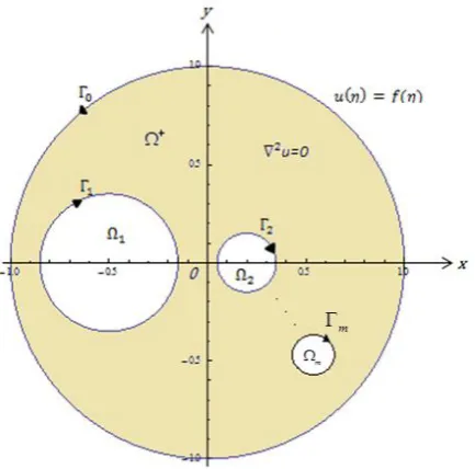
Suppose that  is a multiply connected region of connectivity m1 bounded by simple closed curve Γ = Γ₀∪ Γ₁∪ ⋯ ∪ Γ_𝑚. Let 𝑓 be a piecewise continuous function on Γ and consider the Dirichlet problem as shown in Figure 1.1.

Figure 1.1 A Dirichlet problem in a bounded multiply connected region .

The Dirichlet problem consists in finding 𝑢(𝑥, 𝑦) such that

∇2_{𝑢 = 0}_{for all}_𝑧_in __{, (1.11)} 𝑢(𝜂) = 𝑓(𝜂) for all 𝜂 on Γ. (1.12)

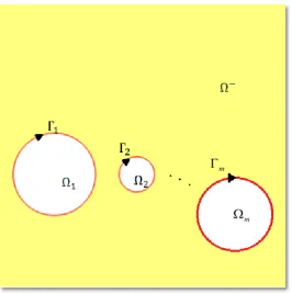
Suppose that  is unbounded multiply connected region of connectivity m while , 1, 2, , ,

j j m

(19)

7

Figure 1.2 An unbounded multiply connected region .

For unbounded, the Dirichlet problem consists in finding 𝑢(𝑧) such that

∇2_{𝑢 = 0}_{for all}_𝑧_in __{, (1.13)} 𝑢(𝜂) = 𝑓(𝜂) for all 𝜂 on Γ, (1.14) 𝑢(𝑧) → 𝑐 , (1.15)

as |𝑧| → ∞ with a constant 𝑐.

Nasser (2007) has developed a new method for solving the Dirichlet problem on bounded and unbounded simply connected regions with smooth boundaries. His method is based on two uniquely Fredholm integral equations of the second kind with the generalized Neumann kernel. Alagele (2012) used Nasser’s method for computing Green’s function on bounded simply connected region by getting a unique solution of interior Dirichlet problem using integral equation approach with the generalized Neumann kernel. Nezhad (2013) computed the Green’s function on unbounded simply connected region by getting a unique solution of the exterior

(20)

8

Dirichlet problem using integral equation approach with the generalized Neumann kernel.

Nasser and Al-Shihri (2013) has introduced a new method for computing conformal mapping of multiply connected regions of high connectivity with fast and accurate result. They used the combination of a uniquely solvable boundary integral equation with the generalized Neumann kernel and the Fast Multipole Method (FMM).

1.3 Statement of the Problem

This research problem is to extend the previous work by Alagele (2012) and Nezhad (2013) for computing the Green’s function from simply connected regions to bounded and unbounded multiply connected regions by getting a unique solution of the Dirichlet problem using integral equation with the generalized Neumann kernel approach. This research also intends to apply FMM in computing Green’s function for regions with connectivity more than three.

1.4 Objectives of the Research

This study embarks on the following objectives:

i. To understand the relationship between Green’s function with Dirichlet problem for bounded and unbounded multiply connected regions.

ii. To study integral equation approach with the generalized Neumann kernel for solving the Dirichlet problem.

(21)

9

iv. To apply FMM for computing Green’s function for bounded multiply connected regions with connectivity more than three and complex geometry.

1.5 Scope of the Research

There are several methods for solving Green’s function such as conformal mapping, integral equation, separation of variables, transform methods, and finite different methods (see Henrici (1986), Embree and Trefethen (1999), Alagele (2012), Nezhad (2013)). This research considers solving the Dirichlet problem on multiply connected regions with smooth boundary using integral equation with generalized Neumann kernel and using combination of a uniquely solvable boundary integral equation with the generalized Neumann kernel and the FMM to compute the Green’s function for bounded multiply connected regions with connectivity more than three and complex geometry.

1.6 Organization of the Report

The report is organized into six chapters. This research begins by studying the various concepts and properties of the Green’s function on simply and multiply connected region. At the same time, the literature review on boundary integral equations with the generalized Neumann kernel for Laplace’s equation in multiply connected regions will be studied in Chapter 2. This chapter explain on how to compute the Green’s function for both bounded and unbounded multiply connected regions.

(22)

10

method with trapezoidal rule leads to a dense and nonsymmetric linear system. The linear system is then solved by the Gaussian elimination method in order 𝑂((𝑚 + 1)3_𝑛3₎_{operations, where}_{𝑚 + 1}_{is the multiplicity of the multiply connected region} and 𝑛 is the number of nodes in the discretization of each boundary component. The computations of the Green’s function are done by using Mathematica software and MATLAB software. Examples for some test regions are presented for better understanding on the concepts of Green’s function for bounded multiply connected regions. Additional conditions are also required for bounded multiply connected regions.

Computing Green’s function for unbounded multiply connected regions is discussed in Chapter 4. After solving the integral equations with generalized Neumann kernel using Nystrӧm method with trapezoidal rule, the linear system is then solved by the Gaussian elimination method and the computations of the Green’s function are again done by using Mathematica software and MATLAB software. Examples for some test regions are presented for better understanding on the concepts of Green’s function for unbounded multiply connected regions. Additional conditions are also required for unbounded multiply connected regions.

In Chapter 5, computing Green’s function on regions with connectivity more than three and regions with corners is presented. By modifying the integral equation for regions with corners and discretize the integral equation by using Nystrӧm method with trapezoidal rule, the linear system that arrived is solved iteratively using GMRES. Each iteration of the GMRES method requires a matrix-vector product which can be computed using the fast multipole method (FMM). For (𝑚 + 1)𝑛 × (𝑚 + 1)𝑛 matrices, the FMM reduces the operations for a matrix-vector product from 𝑂((𝑚 + 1)2𝑛2) to 𝑂((𝑚 + 1)𝑛) where 𝑚 is the number of connectivity and 𝑛 is the number of nodes on each boundary.

(23)

115

REFERENCES

Ahlfors, L. V. (1979). Complex Analysis. International Student Edition. Singapore: McGraw-Hill.

Alagele, M. M. A. (2012). Integral Equation Approach for Computing Green’s Function

on Simply Connected Regions, Universiti Teknologi Malaysia, Johor Bharu: M.Sc. Dissertation.

Al-Hatemi, S. A. A., Murid, A. H. M., and Nasser, M. M. S. (2013a). Solving a Mixed Boundary Value Problem via an Integral Equation with Adjoint Generalized Neumann Kernel in Bounded Multiply Connected Regions. AIP Conf. Proc.

1522: 508-517.

Al-Hatemi, S. A. A., Murid, A. H. M., and Nasser, M. M. S. (2013b). A Boundary Integral Equation with the Generalized Neumann Kernel for a Mixed Boundary Value Problem in Unbounded Multiply Connected Regions. Bound. Value Probl. 2013: 1-17.

Atkinson, K. E. (1997). The Numerical Solution of Integral Equations of the Second Kind. Cambridge: Cambridge University Press.

(24)

116

Bayin, S. S. (2006). Mathematical Methods in Science and Engineering. New York: John Wiley.

Chen, K. (2005). Matrix Preconditioning Techniques and Applications. Cambridge: Cambridge University Press.

Crowdy, D. and Marshall, J. (2007). Green’s Functions for Laplace’s equation in Multiply Connected Domains. IMA J. Appl. Math. 72, pp. 278-301.

Davis, P. J. and Rabinowitz, P. (1984). Methods of Numerical Integration. Orlando: Academic Press.

Duffy, D. G. (2001). Green’s Function with Applications. New York: Chapman & Hall/CRC Press.

Embree, M. and Trefethen, L. N. (1999). Green’s Functions for Multiply Connected Domains via Conformal Mapping, SIAM Rev. 41, pp. 745-761.

Gaier, D. (1964). Konstruktive Methoden der Konformen Abbildung. Springer, Berlin.

Gakhov, F. D. (1966). Boundary Value Problems. English Translation of Russian Edition 1963. Oxford: Pergamon Press.

Greengard, L. and Rokhlin, V. (1987). A Fast Algorithm for Particle Simulations, J. Comput. Phys.. 73: 325-348.

Greengard, L. and Gimbutas, Z. (2012). A MATLAB Toolbox for Fast Multipole Method in Two Dimensions, FMMLIB2D, Version 1.2.

(25)

117

Henrici, P. (1986). Applied and Computational Complex Analysis, Vol. 3. New York: John Wiley.

Helsing, J. and Ojala, R. (2008). On the Evaluation of Layer Potentials Close to Their Sources, J. Comp. Phys., 227: 2899-2921.

Jerri, A. J. (1999). Introduction to Integral Equations with Applications. John Wiley & Sons.

Lee, K. W. (2014). Conformal Mapping and Periodic Cubic Spline Interpolation, Universiti Teknologi Malaysia, Johor Bharu: B. Sc. Thesis.

Liu, Y. (2009). Fast Multipole Boundary Element Method. Cambridge: Cambridge University Press.

Mikhlin, S. G. (1957). Integral Equations, English Translation of Russian edition 1948. Armstrong: Pergamon Press.

Nasser, M. M. S. (2007). Boundary Integral Equations with the Generalized Neumann Kernel for the Neumann Problem. MATEMATIKA, 23: 83-98.

Nasser, M.M.S. (2009a). A Boundary Integral Equation for Conformal Mapping of Bounded Multiply Connected Regions, Computational Methods and Function Theory, 9(1): 127-143.

(26)

118

Nasser, M. M. S. (2009c). The Riemann-Hilbert Problem and the Generalized Neumann Kernel on Unbounded Multiply Connected Regions, The University Researcher (IBB University Journal), 20: 47-60.

Nasser, M. M. S., Murid, A. H. M., Ismail, M. and Alejaily, E. M. A. (2011). Boundary Integral Equations with the Generalized Neumann Kernel for Laplace's Equation in Multiply Connected Regions. Journal in Applied Mathematics and Computation. 217: 4710-4727.

Nasser, M. M. S., Murid, A. H. M., and Al-Hatemi, S. A. A. (2012). A Boundary Integral Equation with the Generalized Neumann Kernel for a Certain Class of Mixed Boundary Value Problem. J. Appl. Math. 2012: 17 pages.

Nasser, M. M. S. and Al-Shihri, F. A. A. (2013). A Fast Boundary Integral Equation Method for Conformal Mapping of Multiply Connected Regions. SIAM J. SCI.

COMPUT., 35(3): A1736-A1760.

Nezhad, S. C. (2013). Integral Equation Approach for Computing Green’s Function on

Unbounded Simply Connected Region, Universiti Teknologi Malaysia, Johor Bahru: M.Sc. Dissertation.

O’Donnell, S. T. and Rokhlin, V. A. (1989). A Fast Algorithm for the Numerical Evaluation of Conformal Mappings. Proc. R. Soc. SIAM J. Sci. Comput. 10(3): 475-487.

Perelomov, A. M. and Zel’dovich, Y. B. (1998). Quantum Mechanics: Selected Topics. Singapore: World Scientific.

Qin, Q. H. (2007). Green’s Function and Boundary Elements of Multifield Materials. Elsevier Science.

(27)

119

Rathsfeld, A. (1993). Iterative Solution of Linear Systems Arising from the Nystrӧm Method for the Doubly-Layer Potential Equation over Curves with Corners.

Maths. Method Appl. Sci., 16: 443-455.

Rokhlin, V. (1985). Rapid Solution of Integral Equations of Classical Potential Theory.

J. Comput. Phys., 60(2): 187-207.

Royston, A. (2008). Notes on the Direc Delta and Green’s Functions. Retrived April 14, 2013, from

http://theory.uchicago.edu/~sethi/Teaching/P221-F2008/DiracsndGreenNotes(08).pdf.

Saad, Y. and Schultz, M. H. (1986). GMRES: A Generalized Minimal Residual Algorithm for Solving Nonsymmetric Linear Systems. SIAM J. Sci. Stat. Comput. 7: 856-869.

Wegmann, R. (2001). Constructive Solution of a Certain Class of Riemann-Hilbert Problems on Multiply Connected Regions. Journal of Computational and Applied Mathematics. 130: 139-161.

Wegmann, R., Murid, A. H. M., and Nasser, M. M. S. (2005). The Riemann–Hilbert Problem and the Generalized Neumann Kernel, J. Comp. Appl. Math. 182: 388-415.

Wegmann, R. and Nasser, M. M. S. (2008). The Riemann–Hilbert Problem and the Generalized Neumann Kernel on Multiply Connected Regions, J. Comp. Appl. Math. 214: 36-57.

(28)

120

Invariants”. Journal of Abstract and Applied Analysis. 2012, 1-29. Hindawi Publishing Corporation.

Yunus, A. A. M., Murid, A. H. M., and Nasser, M. M. S. (2013). Radial Slits Maps of Unbounded Multiply Connected Regions. AIP Conf. Proc.. 1522: 132-139.