Rotation Dynamics of Star Block Copolymers under Shear Flow

Rotation Dynamics of Star Block Copolymers under

Shear Flow

Diego Jaramillo-Cano1, Christos N. Likos1 ID _{Manuel Camargo}2,∗ ID

1 _{Faculty of Physics, University of Vienna, Boltzmanngasse 5, 1090 Vienna, Austria}

2 _{CICBA, Universidad Antonio Nariño - Campus Farallones, Km 18 vía Cali-Jamundí, 760030 Cali, Colombia}

* Correspondence: [email protected]; Tel.: +572-555-1999

Abstract: Star block-copolymers (SBCs) are macromolecules formed by a number of diblock copolymers anchored to a common central core, being the internal monomers solvophilic and the end monomers solvophobic. Recent studies have demonstrated that SBCs constitute a self-assembling building blocks with specific softness, functionalization, shape, and flexibility. Depending on different physical and chemical parameters the SBCs can behave as flexible patchy particles. In this paper, we study the rotational dynamics of isolated SBCs using a hybrid mesoscale simulation technique. We compare three different approaches to analyse the dynamics: the laboratory frame, the non-inertial Eckart’s frame, and a geometrical approximation relating the conformation of the SBC to the velocity profile of the solvent. We find that the geometrical approach is adequate when dealing with very soft systems while in the opposite extreme, the dynamics is best explained using the laboratory frame. On the other hand, the Eckart frame is found to be very general and to reproduced well both extreme cases. We also compare the rotational frequency and the kinetic energy with the definitions of the angular momentum and inertia tensor different from recent publications.

Keywords: Star block-copolymers; hybrid mesoscale simulation technique; rotational frequency; laboratory frame; Eckart frame; geometrical approach

1. Introduction

Polymer solutions have an important role from both fundamental and applied point of views. The addition of a small amount of polymers to a liquid can be use to tune the stability and rheological properties on multiple commercial systems as paints, pharmaceutical products, food and oils. As consequence of the polymer flexibility, a field flow can provoke large conformational changes which in turn influences back the flow field. In this way, to understand the coupling between conformational and dynamical properties of isolated polymers immersed in a field flow is an important first step to elucidate the rheological behaviour of (dilute and semi-dilute) polymer solutions. [1,2]. To date there has been a considerable amount of work on the response of flexible polymers with different architectures (e.g., linear, ring, hyperbranched and star polymers) to shear stress, which has revealed generic and specific properties of such systems. On top of experimental techniques, the development of simulation methods allowing to efficiently couple the solvent particles and monomers, a wide spectrum of behaviors has been found regarding the average deformation and the orientation as a function of the shear rate, as well as, multiple dynamic responses [3–8]. The latter encompass stretching and recoil, tumbling, tank-treading, rupture, and collapse of polymers and ultimately determine the (complex) viscoelastic response of dilute bulk phases.

In this work, we consider the dynamics of isolated star block copolymers (SBCs), which can be exploited as versatile building blocks as they self-assemble into structures with one or multiple clusters of their solvophobic segments, i.e., they behave as self-associating patchy particles, featuring tunable softness, functionalization, shape, and flexibility [9,10]. Recently, the structural properties of isolated SBCs under (linear) shear flow were analysed by means of particle-based multiscale simulations for a wide set of parameters, which include the functionality of the star, the amphiphilicity degree, the solvent quality, and the shear rate. In particular, the formation of attractive patches on the SBC corona

as a function of the shear rate was analysed. Three mechanisms of patch reorganization under shear were identified, which determine the dependence of the patch numbers and orientations on the shear rate, namely, free arms joining existing patches, fusion of medium-sized patches into bigger ones, and fission of large patches into two smaller ones at high shear rates [11].

Along with these studies, the dynamic behaviour of single SBCs must be considered to gain some insights about the influence of these patch rearrangements on the rheology of dilute suspensions. Motivated by a very recent work on the rotational dynamics of star polymers in shear flow [12,13], this work focuses on the dynamics of sheared SBCs analyzed by means of the so-called Eckart frame, which allows to separate pure rotational and vibrational motions. We show that SBCs display a richer structural and dynamical behavior than athermal star polymers in a shear flow and therefore they are also interesting candidates to tune the viscoelastic properties of complex fluids. The rest of the manuscript is organized as follows: in Section2we present the model and the employed tools. In Section3the simulation results are displayed and the ensuing dynamic properties are discussed. Finally, in Section4, we summarize and draw our conclusions.

2. Materials and Methods

2.1. Model and Simulation Method

2.1.1. Coarse-Grained Model for the Star Block Copolymer

As mentioned above, the dynamics of a single SBC immersed in a sheared (Newtonian) solvent is studied by means of a hybrid Multiparticle Collision Dynamics-Molecular Dynamics (MPCD-MD) method, as described in detail in Refs. [10,11]. Briefly, the star polymer and the solvent particles are modeled at a coarse-grained level. Each arm of the SBC is represented as a bead-spring chain having NAinner andNBouter monomers, thereby defining the degree of polymerizationNpol= NA+NB and the amphiphiphilicityα=NB/Npol. The monomers are represented as soft spheres of diameter σand massMinteracting through pair potentialsVAA(r) =VAB(r) =V(r; 0)andVBB(r) =V(r;λ),

where

V(r;λ) =

(

V0(r) + (1−λ)e r≤rc

λV0(r) r>rc.

(1)

Here,V0(r) =4e

h

(σ/r)48−(σ/r)24

i

,rc=21/24σ,ris the monomer-monomer distance, andλis an

attraction-coupling constant. The latter allows us to tune the solvent quality for the B-monomers; as explained in Ref. [10]. In particular, increasing the value ofλenhances the attraction between the

B-monomers. Sufficiently large values of this parameter,λ>0.92, are equivalent to considering that

a homopolymer made of B-monomers is below itsθ-temperature. The bonding between connected

monomers is introduced by a FENE potential

Ubond(r) =−

1 2K R

2

0ln

"

1−

r R0

2#

, (2)

whereK=30(e/σ2)andR0=1.5σ.

2.1.2. Multiparticle Collision Dynamics (MPCD) and Molecular Dynamics (MD)

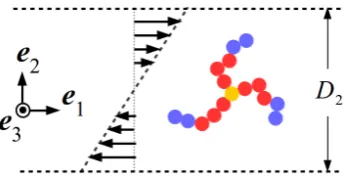
Figure 1.Schematic illustration of the simulation setup, demonstrating the shear (ˆe1), gradient (ˆe2), and vorticity (ˆe3) directions of planar, Couette flow. Yellow, red, and blue spheres correspond respectively to the star core, solvophilic (A type) monomers, and solvophobic (B type) monomers.

cell isρ =5 and their mass ism=M/ρ, serving as the unit of mass of the simulation; a convenient

timescale is defined asτ =

√

mσ2/e. In what follows, we choosem= σ = e = 1, setting thereby

the units of mass, length and energy, respectively; accordingly,τserves as the unit of time. For the

temperatureT, we choose the valuekBT=e/2, wherekBis the Boltzmann constant. The remaining MPCD-parameters were set as follows: the time between collisions is∆tmpcd = 0.1τ, the rotation

angle isχ = 130◦, and the cell sizea = σ, making the presence of two monomers in the collision

cell very unlikely. Lees- Edwards boundary conditions were used to generate a shear velocity field v(x2) =γ˙x2eˆ1, characterized by the shear rate ˙γ, as schematically depicted in Figure1.

In the MD-section of the hybrid technique, time evolution of the monomers follows the Newtonian equations of motion, which are integrated by means of the velocity-Verlet scheme [16] with an integration time step∆tmd=10−3τ. The coupling between the monomers of the SBC and the solvent

particles is achieved during the collision step, in which the former are included as point particles in the evaluation of the center-of-mass velocity of each cell and their velocities are also randomly rotated. This interaction is strong enough to keep the monomers at the desired temperature, once a thermostat for the solvent particles has been introduced, which in the present case corresponds to a cell-level, Maxwell-Boltzmann scaling [17]. During the collision step mass, momentum and energy are conserved, leading to correlations among the particles and giving rise to hydrodynamic interactions. As a dimensionless measure of the shear rate, we consider the Weissenberg numberWi, which is the product of the shear rate with the longest relaxation time of the polymer. For the latter, we take the longest Zimm relaxation timeτZof a polymer withNpolmonomers, which is given by the expression

[5,18]

τZ= ηs

kBT

σ3N_pol3ν, (3)

whereηsis the (MPCD) solvent viscosity andν=3/5 is the Flory exponent for self-avoiding chains.

We obtainτZ'1.3×104τfor the specific choices of the MPCD collision parameters and the value

Npol = 40 employed here. Although we neglect any dependence of the relaxation time on star

functionality and attraction strength along the arms, the results justifya posteriorithe choice of a common relaxation time, in the sense that we are able to obtain results for the shape parameters that mostly collapse on one another when plotted againstWi=γτZ˙ .

We performed a total of 14 independent runs with different initial conditions for each set of parameters{f,α,λ}investigated, covering a broad range ofWi, from the linear (Wi . 1) all the

way to the strongly nonlinear (Wi ' 103) regime. We focus on the following three particular sets of parameters:{f,α,λ} = {12, 0.3, 1.0}(Case 1),{15, 0.5, 1.1}(Case 2) and{18, 0.7, 1.1}(Case 3).

According to our previous study, these parameters represent the typical trends found in regard to the patchiness of the SBCs, namely, no patches are formed, several patches are formed having a small population, and few (one or two) bulky patches are formed [11]. For each run, a preparation cycle of 5×106 MD steps was executed in first place, which was long enough for the SBC to reach its stationary state and then, a production cycle of 1.5×107_{MD steps took place. Depending on the shear}

were saved everyNsave =2×104MD steps during the production cycle. As in this work there exist

various physical systems and they are looked upon at various frames of reference and at different levels of approximations as regards their rotational dynamics, we use in what follows a number of abbreviations, whose meaning is summarized in Table1below.

Table 1.List of shorthands and abbreviations for systems and methods used in this work.

Abbreviation Meaning

Case 1 {f,α,λ}={12, 0.3, 1.0}

Case 2 {f,α,λ}={15, 0.5, 1.1}

Case 3 {f,α,λ}={18, 0.7, 1.1}

LF Laboratory frame

EF Eckart frame

GA Geometric approximation

2.2. Rotational Dynamics

Soft colloids and polymers under shear flow deform and undergo a succession of complex motion patterns, such as tumbling and tank-treading, which are hard to decouple from one another and analyze quantitatively. Recent studies aimed to a better understanding of the complex dynamics of (athermal) star polymers in shear flow, have demonstrated that Eckart’s formalism allows to separates correctly the different characteristic motions of the polymer, i.e., pure rotation, vibration with no-angular momentum and vibrational angular momentum [12,13]. In the following, a brief description of this formalism is given, which will be subsequently employed to analyze our simulation results.

2.2.1. Laboratory frame (LF)

Here, the frame of reference is fixed in space and it is customarily and conveniently chosen in such a way that the first axis lies along the flow direction, the second along the gradient direction and the third along the vorticity direction, as shown in Figure1. Takingrkand˙rkas the position and the velocity of thek-th monomer in the laboratory frame of reference, the total angular momentum of a star polymer with respect to its center of mass is, by definition

L= M Nmon

∑

k=1

∆rk×∆˙rk, (4)

withk=1, . . . ,Nmon= f Npol+1, Nmonthe total number of monomers,∆rk = rk−rcmand∆˙rk = ˙rk−˙rcm. Herercmand˙rcmare, respectively, the position and the velocity of the center of mass, i.e.,

rcm = 1

Nmon

Nmon

∑

k=1

rk. (5)

The time evolution of thek-th monomer position can be evaluated as [12,13,19,20]

˙rk=˙rcm+ (ω×∆rk) +˜vk, (6)

where ˜vkdenotes a purely vibrational motion which is angular momentum-free in the laboratory frame, i.e.,˜vkand∆rkare parallel [cf. Eq. (4)]. The angular frequencyωcan be expressed as

with the components of the moment of inertia tensorJbeing defined as

Jµν=M Nmon

∑

k=1

h

∆r2_kδµν−∆rk,µ∆rk,ν

i

(µ,ν=1, 2, 3), (8)

withδµνthe Kronecker delta andrk,µtheµ-th component of position vector of thek-th monomer. In the case of rigid-body motion, ˜v=0 andωcoincides with the rotational angular velocity.

The full kinetic energyEkinof the sheared polymer results from Eq. (6) and reads as

Ekin = 1

2M

∑

= 1

2Ms˙rcm·˙rcm+ 1

2ω·J·ω+ 1

2M

∑

the translational, rotational, and vibrational contributions to the kinetic energy, respectively. We emphasize, though, that the velocity contribution ˜vk in the motion of a monomer is not the only vibrational contribution but just the one that does not contribute to the (instantaneous) angular momentum; there are, in general, additional vibrational contributions included inω. Therefore,ωis

the apparent angular velocity and it is not possible to separate rotation from vibrational with angular momentum motion within the lab frame.

2.2.2. Eckart frame (EF)

The Eckart’s formalism makes use of a non-inertial frame which co-rotates with the polymer at angular velocityΩ (see Eq. (16) below) [21,22]. The first step to built up the Eckart frame is to choose one initial configuration of the SBC as reference, accompanied by an initial frame of reference spanned by the basis vectors{f1(0),f2(0),f3(0)}. The origin of this frame is located at the center

of mass of the chosen reference configuration of the polymer and, as a matter of convenience, the three axes{f1(0),f2(0),f3(0)}also coincide with the orientation of the laboratory frame. Due to the

choice of the origin, in this system of coordinates the position vectors of the monomers at timet=0,

{ak=∆rk(0);k=1, 2, . . . ,Nmon}, satisfy the relation

Nmon

∑

k=1

ak=0. (10)

This reference configuration is frozen and co-rotates with the Eckard frame of reference, the latter evolving with time as explained below. In the second step of the process, the unit base (column) vectors

{f1(t),f2(t),f3(t)}of the instantaneous Eckart frame are evaluated. To achieve that, the vectors

F_µ(t) =M

∑

k

ak,µ∆rk(t) (µ=1, 2, 3), (11)

are introduced, which are completely defined in terms of the instantaneous positions∆rk(t)and the Cartesian componentsak,µof the reference position vectorsakfor each monomer. In what follows, we drop the explicit time-dependence from the notation of the various vectors. The right-handed triad of unit vectors{f1,f2,f3}is determined as

where the elements of the symmetric (Gram) matrix F are defined as [F]µν = Fµ·Fν and F−1/2F−1/2=F−1. In this way, the position vectorckof thek-th monomer in the co-rotating reference configuration, decomposed onto the unit vectors of the rotating Eckart frame of reference, is given by

ck=

3

∑

µ=1

ak,µfµ, (13)

the coefficientsak,µbeing fixed, time-independent quantities set by the reference configuration, and the triad{f1,f2,f3}depending on time as explained above. In this way, theckareconstantvectors when looked upon from within the rotating Eckart frame and describe the original, rigid configuration.

ᐃt = 250τ

ᐃt = 150τ ᐃt = 200τ

ᐃt = 100τ

ᐃt = 50τ

ᐃt = 0

Wi = 10

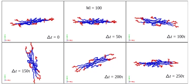
Figure 2. Time evolution of the (fixed) reference configuration in the Eckart’s frame as seen in the laboratory frame for Case 1 andWi=10.

ᐃt = 250τ

Wi = 100

ᐃt = 150τ

ᐃt = 200τ

ᐃt = 100τ

ᐃt = 50τ

ᐃt = 0

Figure 3. Time evolution of the (fixed) reference configuration in the Eckart’s frame as seen in the laboratory frame for Case 1 andWi=100.

ᐃt = 50τ

ᐃt = 200τ

ᐃt = 100τ

Wi = 400

ᐃt = 250τ

ᐃt = 150τ

ᐃt = 0

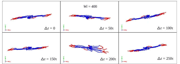
Figure 4. Time evolution of the (fixed) reference configuration in the Eckart’s frame as seen in the laboratory frame for Case 1 andWi=400.

In this frame, the inertia tensor can be written as [21,22]

ˆ

Jµν= M

∑

h

c2_kδµν−ck,µck,ν

i

. (14)

On the other hand, the angular momentum, can be determined by performing a transformation between the laboratory and the Eckart’s frames [22],

ˆL=

3

∑

µ=1

L·fµ

fµ. (15)

As explained in detail in Refs. [21,22], the angular velocity of the Eckart coordinate system is given by

Ω=ˆJ−1_{ˆL, (16)}

providing an expression for the (instantaneous) angular velocityΩof rotation of the Eckart frame. At this point, it is worth noting that the inertia tensorˆJand the angular momentum ˆLdefined above are different from the definitions given in Refs. [13,19,20]. In the present case, both the inertia tensor and the angular momentum are completely defined in terms of variables in the Eckart frame, and consequently so does the kinetic energy, as explained below.

In Eqs. (13) and (14),ck denotes the position vector of thek-th monomer of a (rigid) reference configuration of the polymer measured in the the instantaneous Eckart’s frame. Note that for a rigid molecule,Jin Eq. (8) andˆJin Eq. (14) become equivalent and so doωandΩ[Eqs. (7) and (16)]. In this

frame, the kinetic energy of the polymer can be written as (see AppendixA)

Ekin=

1

2Ms˙rcm·˙rcm+ 1

2Ω·ˆJ·Ω+ 1

2M

∑

2.2.3. Geometrical approach (GA)

A third, complementary approach to estimate the rotational frequency of soft colloids under shear is the so-called geometrical approximation (GA). This is based on two assumptions about the behavior of the polymers in linear shear flow [23,24]. First, it is assumed that the velocity of the monomers is entirely defined by the local, undisturbed velocity profile of the flow according to

∆˙rk'γ˙∆rk,yeˆ1. (18)

Under this assumption the instantaneous angular momentum of the polymer is given by the expression

L= M

∑

∆rk×∆˙rk 'Msγ˙(G23eˆ2−G22eˆ3), (19)

whereGµν= Nmon−1 ∑k∆rk,µ∆rk,νdenotes theµν-component of the gyration tensor, which measures the overall conformation of the SBC. Furthermore, a long-time average is then performed in Eq. (19), whereupon the non-diagonal element of the gyration tensor disappears and thus the average angular momentum has a single component, along the vorticity axis. Finally, it is assumed that the rotation of the SBC takes place mainly around the vorticity axis ˆe3, i.e.,ω1=ω2≈0. Within these approximations ω3=ωGhas a constant value and using Eq. (7) it results into

ωG' −Msγ˙hG22i

hJ33i

=−γ˙ hG22i

hG11i+hG22i

. (20)

Though clear by the construction of the GA, it is worth emphasizing once again that the so-obtained estimate for the angular frequency is a result ofaveraging the polymer motionover very long time intervals while at the same time making the a priori assumption that the instantaneous velocities of the monomers only have a component along the shear direction, dictated by the undistorted solvent velocity profile, see Eq. (18). The final result, Eq. (20), corresponds to the tumbling (rotation) frequency of a rigid body whose shape is similar to the average shape of the SBC and which also have an angular momentum equal to the value given by the mean flow [12,13]. At the same time, however, due to Eq. (18), the estimateωGis also valid for a tank-treading (TT)-type of motion, in which the SBC does

not rotate as a whole but rather the individual arms rotate by tank-treading around the geometrical star center, which remains at rest. This is a different, prototypical type of motion, for which the overall shape of the star remains fixed in time, i.e., no tumbling of the soft colloid as a whole takes place.

3. Results and Discussion

3.1. Global conformation and dynamics

As flexible polymers generically behave in shear flow, the SBC are stretched along the shear direction, compressed along the orthogonal (gradient and vorticity) directions, and exhibit a preferred (average) orientation with respect to the flow. These global features are quantified by the average values

Table 2.The various contributions to the total kinetic energy in both the laboratory and the Eckart frames.

Rotational Vibrational Tu=Vibrational with angular momentum +

without angular momentum Coriolis coupling

Laboratory frame 1₂ω·J·ω M₂ ∑k˜vk·˜vk –

of the gyration tensorGand the orientational angleχG, both of which can be measured experimentally. The latter measures the flow-induced alignment of the polymer and is defined as the angle formed between the eigenvectorˆg1associated with the largest eigenvalue ofGand the flow directionˆe1, and

can be evaluated as

tan(2χG) =

2hG12i

hG11i − hG22i

≡ mG

Wi, (21)

defining this way the orientational resistancemGof the stars in shear flow.

100 101

G

(Wi

)/

G

(0)

α = 0.0 α = 0.3 α = 0.5 α = 0.7

G

10-1 100

G

10-1 100

G

10-1 100 101 102

Wi

100 101

G

(Wi

)/

G

(0)

10-1 100 101 102

Wi

10-1 100

10-1 100 101 102 103

Wi

10-1 100

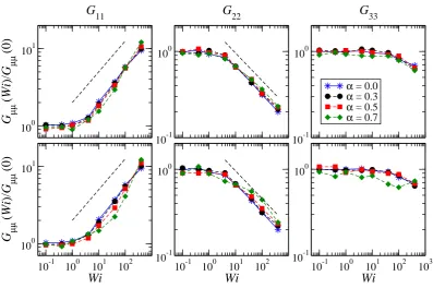
Figure 5. Diagonal components of the (average) gyration tensor of a SBC with f =18,N_pol = 40,

λ = 1.0 (top row), andλ = 1.1 (bottom row). For athermal stars, the scalingsG11 ∼ Wi0.4 and G22∼Wi−0.32are found at highWi.

At low values ofWi, the SBCs are hardly distorted, whereas forWi&10, they become increasingly anisotropic, expanding in the flow direction and shrinking most strongly in the shear direction and in minor proportion along the vorticity axis, as demonstrated by the diagonal components of the gyration tensor in Fig.5. Similarly, Fig.6displays the average alignment angle as a function of the shear rate. At low shear rates (Wi<1) the scaling tan(2χG)∼Wi−0.83is found, while forWi>10 it behaves as tan(2χG)∼Wi−0.3, which is in agreement with previously reported values [5].

The overall (equilibrium) shape of a SBC depends on the number of patches formed and the compactness of the latter, which in turns depends onf,Npol,α, andλ. Depending on the values of

these parameters, three general cases can be recognized. At lowαandλ(α<0.3 andλ<1.0) the star

block copolymers behave very similar ot athermal stars (α=0) with no formation of patches or very

weak, breakable ones (Case 1). On the other opposite limit, at highαandλ(α&0.6 andλ&1.1), the

macromolecule acquires cylindrical symmetry around its principal axis, since it self-assembles into dumbbell-like structures with one or two massive patches (Case 3). At intermediate values ofαandλ,

100 101 102 103

Wi

10-1

100

101

m G

/

Wi

λ = 1.0

100 101 102 103

Wi

10-1

100

101

α = 0.0

α = 0.3

α = 0.5

α = 0.5

λ = 1.1

Figure 6. Reduced orientational resistancemG/Wifor stars with f = 18,Npol =40 and values of

λandαas indicated on the panels. For athermal stars, we findmG/Wi∼Wi−0.83at smallWi, and mG/Wi∼Wi−0.30at largeWi.

in a similar way as athermal stars and then the arms perform tank-treading-like (TT) motions. As the contribution of the attractive interaction increases, patches begin to form and TT rotation is also found, but this time the motion is simultaneously performed by all arms forming the cluster. Finally for highαandλ, the SBC motion closely resembles that of a rigid dumbbell. We will explore, in what

follows, the ways in which these statements based on impressions from simulation snapshots acquire quantitative character through the comparison of characteristic quantities among different reference frames and approximations.

3.2. Reference configuration update

In the original Eckart formalism, the rigid reference configuration of (small) molecules is assumed to be the equilibrium one (all forces on all monomers vanishing) and its dynamics is governed by the time evolution of the positions of the atoms forming the molecule, which are defined by vectorsck, see Eq. (13). Since thermally fluctuating (star) polymers do not have such a rigid equilibrium configuration but rather a multitude of typical configurations related to the given conditions (temperature and shear rate), it is plausible to think that, as the simulation advances, the reference configuration needed to built up the Eckart frame must be updated at regularly spaced numbers of MD steps. The period of updating the characteristic, reference configuration is denoted astEckartand it can vary at will, from a

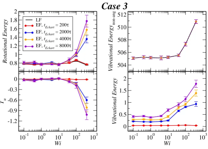
very frequent update of the reference configuration that tries to follow the details of the particle motion to a rare one, for which the average, time-coarsened rotational dynamics of the molecule is captured. In Figures8–10, we compare the behavior of the different contributions to the kinetic energy (see Table2) as a function of the Weissenberg number for different values oftEckart. FortEckart =200τ,

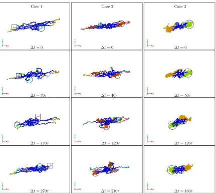
Case 1 Case 2 Case 3

∆t= 0 ∆t= 0 ∆t= 0

∆t= 70τ ∆t= 40τ ∆t= 50τ

∆t= 170τ ∆t= 120τ ∆t= 120τ

∆t= 270τ ∆t= 210τ ∆t= 160τ

1

Figure 7.Representative simulation snapshots displaying the time evolution of the SBC in shear flow for{f,α,λ} ={12, 0.3, 1.0}(Case 1),{15, 0.5, 1.1}(Case 2) and{18, 0.7, 1.1}(Case 3). In Case 1,

individual arms of the star perform tank-treading motion while in Case 3, the star tumbles as a whole. Case 2 presents a tank-treading-like motion but it is performed by both individual and clustered arms. Circles and squares are guides to follow the motion of arms. In all cases,Npol=40 andWi=100. In the panels,∆trepresent the elapsed time from the first configuration inτunits.

frequently, the rotational frequenciesωandΩin the LF and the EF are very similar, i.e.,ω'Ωand

alsoˆJ'J, resulting into the approximate equality of rotational energies:

1

2ω·J·ω' 1

2Ω·ˆJ·Ω (22)

Related to this approximate equality is the vanishingly small value of the kinetic energy contribution Tu, which emerges as the sum of the angular-momentum-carrying contributions and the Coriolis coupling, viz.:

Tu= M

0.9 1.2 1.5 1.8 2.1

Rotational Energy

LF

EF, t_Eckart = 200τ EF, t_Eckart = 2000τ EF, t_Eckart = 4000τ EF, t_Eckart = 8000τ

346 347 348 349

Vibrational Energy

non-ang

10-1 100 101 102 103

Wi

-1.2 -0.9 -0.6 -0.3 0

T u

10-1 100 101 102 103

Wi

0 0.5 1 1.5 2

Vibrational Energy

Case 1

Figure 8.Comparison between the values of the kinetic energy for the Case 1 evaluated in both the lab and Eckart frames at different Eckart times (Table2).

0.8 1 1.2 1.4 1.6 1.8

Rotational Energy

LF

EF, t_Eckart = 200τ EF, t_Eckart = 2000τ EF, t_Eckart = 4000τ EF, t_Eckart = 8000τ

431 432 433 434 435

Vibrational Energy

non-ang

10-1 100 101 102 103

Wi

-1 -0.8 -0.6 -0.4 -0.2 0

T u

10-1 100 101 102 103

Wi

0 0.3 0.6 0.9 1.2 1.5 1.8

Vibrational Energy

Case 2

Figure 9.Comparison between the values of the kinetic energy for the Case 2 evaluated in both the lab and Eckart frames at different Eckart’s times (Table2).

(∆rk ∼= ck) implies the smallness ofuk and of both terms at the right-hand side of Eq. (23) above. Another useful way to look into the quanityTuis to express it as (see AppendixB):

Tu = 1

2ω·J·ω− 1

0.8 1 1.2 1.4 1.6 1.8 2

Rotational Energy

LF

EF, t_Eckart = 200τ EF, t_Eckart = 2000τ EF, t_Eckart = 4000τ EF, t_Eckart = 8000τ

504 506 508 510 512

Vibrational Energy

non-ang

10-1 100 101 102 103

Wi

-1.2 -0.9 -0.6 -0.3 0

T u

10-1 100 101 102 103

Wi

0 0.5 1 1.5 2

Vibrational Energy

Case 3

Figure 10.Comparison between the values of the kinetic energy for the Case 3 evaluated in both the lab and Eckart frames at different Eckart’s times (Table2).

Evidently,Tuis the difference in the rotational energies between the LF and EF and its small value affirms the similarity of the two for frequent updates of the reference configuration in the Eckart frame.

Upon increasing the time intervals between updates of the reference configuration, deviations between the LF and the EF appear in the strongly nonlinear regime,Wi>10. The EF rotational energy grows much higher that its LF counterpart, signaling significant deviations between the (temporally coarse) EF angular velocityΩand its LF-counterpartω. This phenomenon is consistently accompanied

by an increase in the magnitude ofTu as well as an increase in the magnitudes of the velocitiesuk, leading to a growth of the angular-momentum carrying vibrational parts of the energy. The second term at the right-hand side of Eq. (23) is the Coriolis termEC, which can be rewritten in the form

EC = EC,1+EC,2

M

∑

(Ω×ck)·uk = −M

∑

k

(Ω×ρ_k)·uk+M

∑

k

(Ω×∆rk)·uk, (25)

defining the partial terms EC,1andEC,2 with the help of the vectorρ_k = ∆rk−ck, Eq. (A1). The behavior of each term of the Eq. (25) is shown in Fig.11only for case 1 as representative for all other cases as well. FortEckart = 200τ, the Coriolis coupling is close to zero but fortEckart = 400τthe

Coriolis coupling is negative and the contribution related toρ_k, second term in the right Eq. (25), is the

dominant in the Coriolis coupling behavior.

Finally, the vibrational kinetic energy associated with the velocities carrying no angular momentum,Evib= (M/2)∑k ˜vk·˜vk, is very large and its value is essentially independent oftEckart:

10-1 100 101 102 103

Wi

-3.5 -3 -2.5 -2 -1.5 -1 -0.5 0

Coriolis Energy

E_C, t_Eckart = 200τ

E_C,1, t_Eckart = 200τ

E_C,2, t_Eckart = 200τ

E_C, t_Eckart = 8000τ

E_C,1, t_Eckart = 8000τ

E_C,2, t_Eckart = 8000τ

Case 1

Figure 11.The Coriolis coupling for two different values oftEckartfor the case 1 as a function ofWi. For the meaning of the quantitiesEC,EC,1andEC,2, see Eq. (25).

3.3. Angular momentum and angular frequency

We now proceed to our results regarding the angular momenta and frequencies of the SBC motions under shear flow. In Fig. (12) we compare the component of the total angular momentum around the vorticity directionL3in the laboratory frame from Eq. (4) to the value evaluated through

the geometric approximation, Eq. (19). The velocity of the monomers for intermediate values ofWiis well approximated by Eq. (18), i.e., it is mainly determined by the velocity of the fluid, at least in the average sense.

10-1 100 101 102 103

Wi

10-2 10-1 100 101 102 103

L3

Case 1, LF Case 2, LF Case 3, LF Case 1, GA Case 2, GA Case 3, GA

Figure 12.Comparison between the exact value of the componentL3of the angular momentum, Eq. (4), with the one obtained from the geometrical approximation, Eq. (19).

As mentioned before, the definitions of the angular momentum and the inertia tensor for the Eckart’s frame given by Eqs. (4) and (8) are different from the presented ones in Refs. [13,19,20], that is,

L0=M

∑

J0= M

∑

[(∆rk·ck)I−∆rk⊗ck]. (27)

It can be shown that the inertia tensor as defined in the above expression does not meet the symmetry condition in general, i.e.,

∆rk,µck,ν6=∆rk,νck,µ, (28)

which is due to the definition of displacement vectors in the Eckart frameρ_k, see Eq. (A1). In Figs.13–15,

left panels, we demonstrate that employingˆJorJ0leads to different results for the associated rotational frequencies (ΩandΩ0) and the rotational energy. Likewise, it is possible to find the relation between the vectoru0k= (ω−Ω0)×∆rkof Ref. [13] and the quantityukof Eq. (A3) as:

uk=u0k+

Ω0_−Ω ×∆rk

+ (Ω×ρ_k), (29)

10-1 100 101 102 103

Wi

100 101

Rotational Energy

LF

EF, t_Eckart = 200τ EF, t_Eckart = 2000τ EF, t_Eckart = 4000τ EF, t_Eckart = 8000τ EF', tEckart = 200τ EF', t_Eckart = 2000τ EF', t_Eckart = 4000τ EF', t_Eckart = 8000τ

Case 1

10-1 100 101 102 103

Wi

10-2 10-1 100

Reduced angular frequency

LF

EF, t_Eckart = 200τ EF, t_Eckart = 2000τ EF, t_Eckart = 4000τ EF, tEckart = 8000τ GA

Case 1

Figure 13.Left panel: Rotational energy (LF→ 1₂ω·J·ω, EF→ 1₂Ω·ˆJ·Ω, EF0→ 1₂Ω0·J0·Ω0) for two different schemes for the Eckart frame as a function of the Weissenberg numberWi. Right panel: reduced angular frequency for case 1 (LF→ω/ ˙γ, EF→Ω/ ˙γ, GA→ωG/ ˙γ) as a function ofWifor

different Eckart times. EF represents our analytical procedure, whereas EF0represents the analytical procedure from Refs. [13,19,20].

10-1 100 101 102 103

Wi

100 101

Rotational Energy

LF

EF, tEckart = 200τ EF, tEckart = 2000τ EF, t_Eckart = 4000τ EF, t_Eckart = 8000τ EF', t_Eckart = 200τ EF', t_Eckart = 2000τ EF', t_Eckart = 4000τ EF', t_Eckart = 8000τ

Case 2

10-1 100 101 102 103

Wi

10-2 10-1 100

Reduced angular frequency

LF

EF, tEckart = 200τ EF, tEckart = 2000τ EF, t_Eckart = 4000τ EF, t_Eckart = 8000τ GA

Case 2

Figure 14.Same as Figure13but for Case 2.

Results for the angular frequency as a function ofWiand the dependence of this function on the frame of reference as well as on the configuration update timetEckartare shown in Figs.13–15, right

for sufficiently long updating intervalstEckart. It is interesting to confirm that, indeed, the Eckart

rotation frequencies are enclosed by the extreme cases, i.e., the geometric approximation as an upper bound and laboratory frame as a lower bound. AstEckartgrows, the Eckart rotation frequencies move

from the LF- towards the GA-curves, confirming the fact that at coarse time scales the stars, at least for Cases 1 and 2, can be thought of as soft colloids with a tank-treading type of motion of the polymers in their interior.

10-1 100 101 102 103

Wi

100 101

Rotational Energy

LF

EF, t_Eckart = 200τ EF, t_Eckart = 2000τ EF, t_Eckart = 4000τ EF, t_Eckart = 8000τ EF', t_Eckart = 200τ EF', tEckart = 2000τ EF', tEckart = 4000τ EF', t_Eckart = 8000τ

Case 3

10-1 100 101 102 103

Wi

10-2 10-1 100

Reduced angular frequency

LF

EF, t_Eckart = 200τ EF, t_Eckart = 2000τ EF, t_Eckart = 4000τ EF, t_Eckart = 8000τ GA

Case 3

Figure 15.Same as Figure13but for Case 3.

10-1 100 101 102 103

Wi

10-2 10-1 100

Reduced angular frequency

GA ~Wi-0.75 LF ~Wi-1.00 EF ~Wi-0.80 Case 1

10-1 100 101 102 103

Wi

10-2 10-1 100

Reduced angular frequency

GA ~Wi-1.05 LF ~Wi-1.55 EF ~Wi-1.35 Case 3

Figure 16.The reduced angular frequencies for Case 1 (left) and Case 3 (right) evaluated at the LF, the GA and the EF with the longest Eckart time employed,tEckart=8000τ.

Case 3 seems exceptional, in the sense that the angular frequency evaluated in the EF appears to be almost independent of the parametertEckart and always very close to the LF-result. This is

an indication of the fact that, contrary to the other two cases, these star block copolymers do not behave as tank-treading soft colloids. On the contrary, and consistently with their rather compact, elongated, dumbbell-shape, they rotate similarly to rigid prolate ellipsoids under constant shear flow. In particular, the GA-assumption of isolated monomers, each of which is carried through the solvent with the local velocity of the streaming solvent is not valid in this case, since the bulky patches at the ends of these self-associated stars act as compact objects creating backflow and strongly affecting the solvent. To emphasize the difference between Case 1 and Case 3, in Fig.16we plot the angular frequencies for the two limiting frames, LF and GA, together with the EF-result at the longest Eckart time,tEckart =8000τ. As it can be seen, whereas for Case 1 the EF is very close to the GA and far away

4. Conclusions

In this work, we analyze the rotational dynamics of an isolated star-shaped block copolymers under shear flow for three representative set of parameters, i.e., a very flexible system (case 1), an intermediate flexible-rigid system (case 2) and finally a rather rigid system (case 3). Motivated by very recent studies on polymer dynamics [12,13], we explored the quantitative predictions emerging from the employ of the Eckart frame formalism, and compare them to the resulting ones from two different approaches (lab frame and geometrical approach). Additionally, we performed an analysis of each term in the kinetic energy and the contributions of the various kinetic terms to it.

Based on the original formalism [21], we found some differences with respect to the treatment presented in Refs. [13,19,20], which have consequences on the analytical definitions of the inertia tensor and the angular momentum within the Eckart’s frame (Eqs. (27), (26) and (14), (15)). As consequence, we obtained different analytical approximations for the total kinetic energy and for the numerical value for the rotational frequency of the SBC, which we express using strictly the Eckart’s variables. It is important to note that both treatments reproduce correctly the results for the laboratory frame for small updating timetEckart(tEckart ∼200τ); however fortEckart >200τ, we found differences between

both treatments, particularly for the rotational energy term. ForWi<10, we found that the rotational energy is independent oftEckart, which is not the case in Ref. [13]. Additionally, both the rotational

energy and frequency found in Ref. [13] are larger than the outcomes from our treatment.

The main result concerns the behavior of the associated rotational frequencyΩat high shear rate (Wi>100) for the three different systems. We found that for all casesΩis bounded by the rotational frequencies obtained in the lab frame (ω) and from the geometric approximation (ωG), specifically

ω .Ω .ωG. For the third case, i.e., self-assembled, dumbbell-like SBC,Ω ≈ωindependently of

the updating timetEckart, demonstrating that the rotation frequency mainly corresponds to tumbling

motion of the SBC induced by the shear flow. On the other hand, for case 1, which is closely related to athermal star polymers, the results obtained from the geometrical approximation are consistent with the Eckart frame only for long enoughtEckart; therefore, the geometrical approximation only captures

the average, time-coarsened tank-treading rotational frequency of the polymer. These results agree with the obtained for athermal stars with smaller polymerization degree (Npol =6), for which was

found that the vibrational angular momentum has a larger contribution for softer polymers [13]. The dynamics of the case 2 is richer; although this system features four patches in average [11], the shear causes those patches to break and to cluster over and over again. Therefore, here the rotational frequency results from the average of the tank-treading motion of free and clustered arms. It remains to establish a more detailed description regarding the statistic of the typical times between break-up and rejoin events, which shed light on their influence on the rheology of semi-dilute suspensions, in particular on the expected shear thinning behavior and how it can be tuned by the amphiphilicity and the solvent quality [1].

Appendix A. Kinetic energy in the Eckart frame

The monomer displacement vectors compatible with the Eckart’s frame are defined as [13,21,22]

ρ_k=∆rk−ck, (A1)

and therefore the time evolution of thek-th monomer in the Eckart’s frame results in [21,22]

˙rk=˙rcm+c˙k+ρ˙_k =˙rcm+ (Ω×ck) +ρ˙_k. (A2)

Definingρ˙_k = ˜vk+ukwith,

the time evolution equation can be written as

˙rk=˙rcm+ (Ω×ck) + ˜vk+uk. (A4)

We note that fortEckart =200τ,ω≈Ω,∆rk ≈ ckanduk ≈0(see Section3.2). Concomitantly with Eq. (A4), the resulting kinetic energy is

M

2

∑

2 ˙rcm·˙rcm+ M

2

∑

2

∑

2

∑

˙rcm·(Ω×M

∑

ck) +˙rcm·M

∑

˜vk+˙rcm·M

∑

uk+ (A5)

M

∑

(Ω×ck)· ˜vk+M

∑

k

(Ω×ck)·uk+M

∑

k

˜vk·uk.

Since the following equalities hold [21,22],

M

∑

ck=0, (A6)

M

∑

∆˙rk =MΩ×

∑

ck+M

∑

˜vk+M

∑

uk =0→M

∑

uk=0, (A7)

and the definition ofukimplies

M

∑

˜vk·uk =M

∑

˜vk·(ω×∆rk)−M

∑

˜vk·(Ω×ck) =−M

∑

˜vk·(Ω×ck), (A8)

then the kinetic energy can be expressed as in Eq (17).

Appendix B. Explicit calculation ofTu

Starting with the definition of vectoruk, Eq. (A3), the energyTu(Table2) can be written as,

Tu = M

2

∑

∑

= M

2

∑

∑

Tu = 1

2 ω·J·ω+Ω·ˆJ·Ω−2M(ω×∆rk)·(Ω×ck)

+ M(ω×∆rk)·(Ω×ck)−Ω·ˆJ·Ω

, (A10) so that

Tu = 1

2ω·J·ω− 1

2Ω·ˆJ·Ω. (A11)

Appendix C. Rotation frequencies

We show results for all components of the angular frequency. In general, we find that the angular velocity in the vorticity axis is dominant in the angular frequency vector, especially asWigrows. The vorticity componentω3approaches a constant value at high values ofWior even shows a decrease

10-1 100 101 102 103 Wi 10-9 10-8 10-7 10-6 10-5 10-4 10-3 | ωµ |, | ω |

|ω1|, tEckart = 200τ

|ω2|, tEckart = 200τ

|ω₃|, t_Eckart = 200τ |ω|, t_Eckart = 200τ |ω₁|, t

Eckart = 8000τ

|ω2|, tEckart = 8000τ

|ω3|, tEckart = 8000τ

|ω|, t_Eckart = 8000τ

Case 1

10-1 100 101 102 103

Wi 10-9 10-8 10-7 10-6 10-5 10-4 10-3 | ωµ |, | ω |

|ω1|, tEckart = 200τ

|ω2|, tEckart = 200τ

|ω₃|, t_Eckart = 200τ |ω|, t_Eckart = 200τ |ω₁|, t

Eckart = 8000τ

|ω2|, tEckart = 8000τ

|ω3|, tEckart = 8000τ

|ω|, t_Eckart = 8000τ

Case 2

10-1 100 101 102 103

Wi 10-9 10-8 10-7 10-6 10-5 10-4 10-3 | ωµ |, | ω |

|ω₁|, t_Eckart = 200τ |ω₂|, t

Eckart = 200τ

|ω₃|, t

Eckart = 200τ

|ω|, t_Eckart = 200τ |ω1|, tEckart = 8000τ

|ω₂|, t_Eckart = 8000τ |ω₃|, t_Eckart = 8000τ |ω|, t

Eckart = 8000τ

Case 3

Figure A1.Values of the average magnitudes of the components of the angular velocity,|ωµ|, and the magnitude of the whole vector,|ω|, for case 1 as a function ofWifor two differents values of thetEckart as indicated in the legend, for Cases 1,2, and 3.

Acknowledgments: The authors thank support by the European Training Network COLLDENSE (H2020-MCSA-ITN-2014, Grant No. 642774). M.C. is grateful to VCTI-UAN (Project 2016202) and Colciencias (Grant FP44842-014-2015). Computer time at the Vienna Scientific Cluster (VSC) is gratefully acknowledged.

Author Contributions: D.J. and C.N.L. conceived and designed the study; D.J. performed the MPCD+MD simulations; D.J. and M.C. analyzed the data; D.J., M.C. and C.N.L. wrote the paper.

Conflicts of Interest:The authors declare no conflict of interest. The founding sponsors had no role in the design of the study; in the collection, analyses, or interpretation of data; in the writing of the manuscript, and in the decision to publish the results.

References

1. Winkler, R.G.; Fedosov, D.A.; Gompper, G. Dynamical and rheological properties of soft colloid suspensions. Curr. Opin. Colloid Interface Sci.2014,19, 594–610.

2. Vlassopoulos, D.; Cloitre, M. Tunable rheology of dense soft deformable colloid. Curr. Opin. Colloid Interface Sci.2014,19, 561–574.

3. Winkler, R. Semiflexible polymers in shear flow. Phys. Rev. Lett.2006,97, 128301.

4. Dalal, I.S.; Albaugh, A.; Hoda, N.; Larson, R.G. Tumbling and deformation of isolated polymer chains in shearing flow. Macromolecules2012,45, 9493–9499.

5. Ripoll, M.; Winkler, R.G.; Gompper, G. Star polymers in shear flow. Phys. Rev. Lett.2006,96, 188302. 6. Yamamoto, T.; Masaoka, N. Numerical simulation of star polymers under shear flow using a coupling

method of multi-particle collision dynamics and molecular dynamics. Rheologica Acta2015,54, 139–147. 7. Nikoubashman, A.; Likos, C.N. Branched polymers under shear. Macromolecules2010,43, 1610–1620. 8. Chen, W.; Li, Y.; Zhao, H.; Liu, L.; Chen, J.; An, L. Conformations and dynamics of single flexible ring

polymers in simple shear flow.Polymer2015,64, 93–99.

10. Rovigatti, L.; Capone, B.; Likos, C.N. Soft self-assembled nanoparticles with temperature-dependent properties.Nanoscale2016,8, 3288–3295.

11. Jaramillo-Cano, D.; Formanek, M.; Likos, C.; Camargo, M. Star block-copolymers in shear flow. J. Phys. Chem. B2018,122, 4149–4158.

12. Sablic, J.; Praprotnik, M.; Delgado-Buscalioni, R. Deciphering the dynamics of star molecules in shear flow. Soft Matter2017,13, 4971–4987.

13. Sabli´c, J.; Delgado-Buscalioni, R.; Praprotnik, M. Application of the Eckart frame to soft matter: rotation of star polymers under shear flow.Soft Matter2017,13, 6988–7000.

14. Malevanets, A.; Kapral, R. Mesoscopic model for solvent dynamics. J. Chem. Phys.1999,110, 8605–8613. 15. Malevanets, A.; Kapral, R. Solute molecular dynamics in a mesoscale solvent. J. Chem. Phys. 2000,

112, 7260–7269.

16. Frenkel, D.; Smit, B.Understanding Molecular Simulation: From Algorithms to Applications; Academic Press, 2001.

17. Huang, C.C.; Chatterji, A.; Sutmann, G.; Gompper, G.; Winkler, R.G. Cell-level canonical sampling by velocity scaling for multiparticle collision dynamics simulations.J. Comput. Phys.2010,229, 168–177. 18. Doi, M.; Edwards, S.F.The Theory of Polymer Dynamics; Oxford University Press, 1986.

19. Park, S.; Moon, J.; Kim, M. Rotational energy analysis for rotating–vibrating linear molecules in classical trajectory simulation. J. Chem. Phys.1997,107, 9899–9906.

20. Rhee, Y.; Kim, M. Mode-specific energy analysis for rotating-vibrating triatomic molecules in classical trajectory simulation. J. Chem. Phys.1997,107, 1394–1402.

21. Eckart, C. Some studies concerning rotating axes and polyatomic molecules. Phys. Rev.1935,47, 552. 22. Louck, J.; Galbraith, H. Eckart vectors, Eckart frames, and polyatomic molecules.Rev. Mod. Phys.1976,

48, 69.

23. Aust, C.; Hess, S.; Kröger, M. Rotation and deformation of a finitely extendable flexible polymer molecule in a steady shear flow.Macromolecules2002,35, 8621–8630.