Interactive Image Segmentation Using
Dynamic Bayesian Network
Saranya
1, Esther
2, Sheela
3, S.Venshiba
41UG Student, Department of ECE, Rajas Engineering College, Vadakkangulam, India
2UG Student, Department of ECE, Rajas Engineering College, Vadakkangulam, India
3UG Student, Department of ECE, Rajas Engineering College, Vadakkangulam, India
4UG Student, Department of ECE, Rajas Engineering College, Vadakkangulam, India
ABSTRACT: Segmenting semantically meaningful whole objects from images is a challenging problem, and it becomes especially so without higher level common sense reasoning. In this project, we present an interactive segmentation framework that integrates image appearance and boundary constraints in a principled way to address this problem. In particular, we assume that small sets of pixels, which are referred to as seed pixels, are labeled as the object and background. The seed pixels are used to estimate the labels of the unlabeled pixels using Dirichlet process multiple-view learning, The boundary extraction problem is formulated as a Dynamic Bayesian network and the novel approach to the Dirichlet Mixtures with state pruning is used to find the optimal boundary in a robust and efficient manner based on the extracted external and internal local costs, thus handling much inexact user boundary donations than existing methods.
I. INTRODUCTION
Despite many years of research, unsupervised image segmentation techniques without human interaction still do not produce satisfactory results. Fully automated segmentation is an ill-posed problem due to the fact that there is neither a clear definition of a correct segmentation nor an objective measure of the goodness of a segment. In order to do semantically meaningful image segmentation, it is essential to take a priori information about the image into account. This issue has been addressed in the literature as interactive image segmentation, which takes human inputs through a set of strokes or a tri map that provides labeled pixels (called seeds)for the objects and backgrounds and aims to produce semantically meaningful object regions. Although interactive segmentation has drawn much attention little existing work has systematically studied the problem of insufficient seeds. For instance, in order to perform interactive segmentation on the image, when there is no seed at the trunk of the tree, a typical interactive segmentation method would fail to segment it as part of the tree. The reason is that the trunk and leaves have very different color components, and therefore, there is no sufficient cue for the seeds on the leaves to influence the segmentation decisions on the trunk. A partial solution to this problem is through active learning a framework that allows the learning algorithm to ask for informative labeled examples at certain costs. However, additional labeled information through user interaction is not always available. Thus, we propose an automatic approach in order to address the issue when fewer than enough seeds are provided. Such situations might happen in real applications where an insufficient amount of seeds are given by an amateurish user.
II. RELATED WORKS
2.1 Nonlinear models using Dirichlet process mixtures:
Peter Orbanzand Joachim M. BuhmannInstitute of Computational Science, ETH ZurichEuropean Conference on Computer Vision (ECCV), 2006, the study of them include the following points:
is linear. However, the performance of such a model depends on the appropriateness of these assumptions. Poor performance may result from assuming wrong distributions, or regarding relationships as linear when they are not. In this paper, we introduce a new model based on a Dirichlet process mixture of simple distributions, which is more flexible in capturing nonlinear relationships. A Dirichlet process, D(G0,g), with baseline distribution G0 and scale
parameter g, is a distribution over distributions. Ferguson introduced the Dirichlet process as a class of prior distributions for which the support is large, and the posterior distribution is manageable analytically.Using the Polyaurn scheme, Blackwell and Macqueen showed that the distributions sampled from a Dirichlet process are discrete almost surely. The idea of using a Dirichlet process as the prior for the mixing proportions of a simple distribution (e.g., Gaussian) was first introduced by Antoniak. In this paper, we will describe the Dirichlet process mixture model as a limit of a finite mixture model.Suppose exchangeable random values y1, ... , yn are drawn independently from some
unknown distribution. We can model the distribution of y as a mixture of simple distributions, with probability or density function.
2.2 Interactive image segmentation using probabilistic hyper graphs:
Pablo Arbel´aez University of California,Berkeley, CEREMADE, UMR CNRS 753 Universit´e Paris Dauphine,75775 Paris, France in 2006 concluded interactive image segmentation using probabilistic hyper graph as,Unsupervised image segmentation techniques without human interaction still do not produce satisfactory results. Fully automated segmentation is known to be an ill-posed problem due to the fact that there is neither a clear definition of a correct segmentation no ran objective measure of the goodness of a segment. In order to do semantically meaningful image segmentation, it is essential to take a priori information about the image in to account. Such information, for example, can be provided by the user through a set of strokes labelling the pixels in an image. This issue has been addressed in the literature as interactive image segmentation, which has been successfully used in snakes, intelligent scissors and interactive graph-cuts. Our approach is in line with a more recent direction of interactive image segmentation which exploits graph-based machine learning. Image segmentation shares the basic assumption of graph-based function estimation where the target function to estimate is smooth with respect to the affinity graph constructed from the image content. Hence, segmentation becomes a labeling problem to which graph-based learning methods can be applied. In the last several years, machine learning researchers have introduced various methods for graph- based learning including but not limited to graph-min cuts, harmonic energy minimization, Laplacian Eigen maps and manifold regularization.
In this paper, different from the traditional graph-based approaches, we use the hyper graph, which is a generalization of a graph, as the underlying model for the image content. In a hyper graph, the edges (known as hyper edges) may connect an arbitrary number of vertices. Hyper graphs have recently been used in various applications including but not limited to image processing, image segmentation and VLSI application. As an image modeling tool, compared to standard graphs that model pairs of pixels as their edges, hyper graphs can model image patches as their hyper edges. This property lets hyper graphs define higher-order relations among pixels and provide a means to exploit user-supplied labels for labeling unlabeled pixels. Under this formalism, we use a hyper graph based interpolation as our main segmentation algorithm, and provide its equivalence using an iterative update rule.
III. SYSTEM OVERVIEW
3.1 Preprocessing:
3.2 Feature extraction:
Our implicit assumption is that pixels within the same object, although may have distinct appearance features (e.g., colors), share similar spatial relations to salient boundaries. In particular, we consider the multiple-view pixel representations,
fig : Block Diagram of Proposed System
namely, the color- and boundary-related features, and
effectively exploit these two complementary views to perform segmentation better than what either of them could achieve. The two complementary features of a super pixel are image appearance feature represented by mean RGB color values at constituent pixels and boundary feature represented by the diffusion signature vector.
3.2.1 Boundary features: Diffusion signature vector
The two complementary features of a superpixel are image appearance feature represented by mean RGB color values at constituent pixels and boundary feature represented by the diffusion signature vector that will be discussed next. To start with, salient boundaries in an image are described by assigning boundary probabilities to image pixels. Intuitively, the boundaries internal to semantic objects are weaker in strength (i.e., the mean value of boundary probabilities) than the external ones that outline objects. Such a claim is validated by an empirical analysis on two common datasets, namely, GrabCut dataset for single objects and LHI dataset for multiple objects with object-level segmentation ground truth.
3.3 Fuzzy C-means clustering
far away from the center of a cluster will have a low degree of belonging or membership to that cluster.
3.4 Dirichlet process
The classification method we use is akin to the Dirichlet process mixture models (DPMMs). Unlike Gaussian mixtures, DPMMs allow for automatic determination of the number of components.
𝑥𝑖|𝜃𝑖~ (𝜃𝑖) , 𝜃𝑖|𝐺~𝐺, 𝐺~𝐷(𝐺𝑜, 𝛾)
where xi Is a datapoint, θi is the model parameter associated with xi, ∫() is a parametric density function (e.g.,
multivariate Gaussian), and G is a distribution over parameters, which is drawn from a Dirichlet process D with a base distribution Go and a scale parameter γ . In practice, however, distribution G can be integrated out, resulting in a
closed-form conditional distribution of model parameters.
𝜃𝑛+1|𝜃1, … … … 𝜃𝑛~
1
𝑛 + 𝛾 𝑛 𝛿(
𝑖−1 𝜃𝑖 )
+ 𝛾
𝑛 + 𝛾𝐺𝑜
where δ(Ө) denotes the Dirac delta distribution concentrated at Ө.
3.5 Dynamic Bayesian network:
IV. TECHNIQUE - DIRICHLET PROCESS MIXTURES
Here, we overview some important properties of Dirichlet process mixtures, and we proceed by describing the base model in our framework built on Dirichlet process sampling and clustering. Dirichlet process is a prior commonly used in non-parametric Bayesian modeling. In other words, a Dirichlet process is a distribution over distributions, such that each draw from the process is itself a distribution.
Another way to think of a Dirichlet process is as an infinite-dimensional generalization of the Dirichlet distribution. The Dirichlet distribution returns a finite-dimensional set of probabilities (for some size K, specified by the parameters of the distribution), all of which sum to 1. This can be thought of as a finite-dimensional discrete distribution; i.e. a Dirichlet distribution can be thought of as a distribution over K-dimensional discrete distributions. Imagine generalizing a symmetric Dirichlet distribution, defined by a dimension and concentration parameter α/K, to an infinite set of probabilities; the resulting distribution over infinite-dimensional discrete distributions is called the stick-breaking process. Imagine then using this set of probabilities to create an infinite-dimensional mixture model, with each separate probability from the set associated with a mixture component, and the value of each component drawn separately from a base distribution H; then draw an infinite number of samples from this mixture model. The infinite set of random variables corresponding to the marginal distribution of these samples is a Dirichlet process with parameters H and α.
Consider a simple mixture model: Ө1,….k ~ H()
β ~ Dirichlet(α/k,...α/k) z1,….N ~ Categorical(β)
xi=1,….N ~ F(Өi)
This is a basic generative model where the observations x1,….N are distributed according to a mixture of K components,
where each component is distributed according to a single parametric family F(Ө) but where different components have different values of Ө, which is drawn in turn from a distribution H. Typically, H will be the conjugate prior distribution of F. In addition, the prior probability of each component is specified by β, which is a size-K vector of probabilities, all of which add up to 1.
the distribution of prices in that neighborhood. Then the parameter Ө will be a vector of two values, a mean drawn from a Gaussian distribution and a variance drawn from an inverse gamma distribution, which are the conjugate priors of the mean and variance, respectively, of a Gaussian distribution.Meanwhile, if the observations are words and the K components represent different topics, then F might be a categorical distribution over a vocabulary of size V, with unknown frequencies of each word in the vocabulary, specifying the distribution of words in each particular topic. Then the parameter Ө will be a vector of V values, each representing a probability and all summing to one, drawn from a Dirichlet distribution, which is the conjugate prior of the categorical distribution.Now imagine we consider the limit as K→∞. Conceptually this means that we have no idea how many components are present. The result will be as follows: Ө1,….∞ ~ H()
β ~ Stick(1,α) z1,….N ~ Categorical(β)
xi=1,….N ~ F(Өi)
In this model, conceptually speaking there are an infinite number of components, each with a separate parameter value, and a correspondingly infinite number of prior probabilities for each component, drawn from a stick-breaking process. Note that a practical application of such a model would not actually store an infinite number of components. Instead, it would generate the component prior probabilities one at a time from the stick-breaking process, which by construction tends to return the largest probability values first. As each component probability is drawn, a corresponding parameter value is also drawn. At any one time, some of the prior probability mass will be assigned to components and some unassigned. To generate a new observation, a random number between 0 and 1 is drawn uniformly, and if it lands in the unassigned mass, new components are drawn as necessary (each one reducing the amount of unassigned mass) until enough mass has been allocated to place this number in an existing component. It can be shown that
where (k=1,….K) is a particular value of Zi and ηk is the number of times a topic assignment in the set {z1,…zi-1}has
the value k, i probability of assigning an observation to a particular component is roughly proportional to the number of previous observations already assigned to this component.Now consider the limit as K→∞. For a particular previously observed component K,
Now imagine further that we also marginalize out the component assignments Z1,….,N , and instead we look directly at
the distribution of ϕi= Өi. Then, we can write the model directly in terms of the Dirichlet process:
G ~ DP1(H,α)
Φ 1,….N ~ G
xi=1,….N ~ F(Өi)
DP1 represents one view (the distribution-centered view) of the Dirichlet process as producing a random,
infinite-dimensional discrete distribution G with values drawn from H.
An alternative view of the Dirichlet process (the process-centered view), adhering more closely to its definition as a stochastic process, sees it as directly producing an infinite stream of ϕ values. Notating this view as DP2, we can write
the model as
Φ1,…….N ~ DP2(H,α)
xi=1,….N ~ F(Өi)
4.1 DPMM
The classification method we use is akin to the Dirichlet process mixture models (DPMMs). Unlike Gaussian mixtures, DPMMs allow for automatic determination of the number of components. In a DPMM, a data point is drawn according to the Polya urn scheme
𝑥𝑖|𝜃𝑖~ (𝜃𝑖) , 𝜃𝑖|𝐺~𝐺, 𝐺~𝐷(𝐺𝑜, 𝛾)
Where xi is a datapoint, θi is the model parameter associated with xi, ∫( ) is a parametric density function (e.g.,
closed-form conditional distribution of model parameters.DPMMs apply to clustering problems involving any given parametric mixture densities
𝑝 𝑥 = 𝜔 (𝑥|𝜑𝑘)
Ώ
𝑘−1
with k components. Given a set of observed data points xi, sampling the DPMM will result in a set of estimates Өi for
the corresponding component parameters for each data point xi.The component parameters for the component are
denoted as. It follows that, where is the component index for data point. Grouping identical component parameter estimates implicitly determines the assignments of the data to components. The mixture weights in the parametric case are analogous to the component sizes determined by a DPMM.
4.2 DPMLM
The single-view case of our model is based on the Dirichlet process multinomial logistic model (DPMNL). In this model, a component refers to a group of salient features corresponding to the image structures in our case. A single component might contain both the object and background pixels, which is modeled by a multinomial logistic function between an input vector and an output class y. Specifically, each component in the mixture model has parameters Φ=(α,β,γ,θ). The distribution of xi within the component follows a Gaussian model ή=(μ,ε) where μ is the mean vector
and ε is the diagonal covariance matrix with elements ζt2 .The distribution of y given x within the component follows
𝑃 𝑦 − 𝑗 𝑥, ∝, 𝛽 − exp 𝛼2− 𝑥𝑝 𝛽1 / exp 𝛼2− 𝑥𝑝 𝛽1
𝑘−1
where J is the number of segments (α,β) is equal to 2 for single object segmentation and α and β are regression parameters. Here, we illustrate the graphical model representation of DPMNL, which reveals the interdependence among parameters θ and variables. To be more accurate, model parameters are sampled from a distribution G that is drawn from a Dirichlet process, D(Go,γ) where Go is a base distribution over model parameters and γ is a scale
parameter. Go’s parameters may depend on higher level hyper parameters. For simplicity, we use fixed distributions for
Go. On the other hand, x and y are drawn according to their distributions with the sampled model parameters.
In contrast to discriminative multinomial logistic models, DPMNL is a generative model since it estimates the joint distribution of the input vector and its label as
P(x,y)=P(x)P(y|x).
Generative models have several advantages over discriminative models. First, generative models can augment small quantities of seeding pixels with large quantities of unlabeled pixels, which are especially useful for producing semantic segments. Second, generative models can readily handle the compositionality of an object as a meaningful sub-component, whereas standard discriminative models need to see all combinations of possibilities during the training phase.
4.3 DPMVL
Here, we describe the proposed extensions to DPMNL to accommodate the use of multiple views in image segmentation, along with related algorithms for parameter learning and inference in the extended model. The resulting methodology is referred to as DPMVL.
4.4 Model Description
mean RGB values of constituent pixels) and the diffusion signature vector that will be covered, and is the segment label. The parameters superscripted with 1 and 2 are associated with the two views, respectively. During the assignment of data to components, the two views cooperate to decide the probabilities used for sampling. In parameter re-estimation, parameters associated with each view inside a component are separately updated, and weight parameters {η,ν} are decided using the interaction between the two views in order to appropriately trade them off. The extended set of component parameters is therefore Φ= (μ1, μ2, α1, α2, β1, β2, ν, η).
More specifically, within each component, class label y follows a multinomial logistic model given the input vectors from the two views and the component parameters.We define g = P(y-1|x1), P(y-1|x2)-T.Therefore
𝑃 𝑦 = 𝑗 𝑥1, 𝑥2, ∝, 𝛽, 𝜏, 𝛾 = exp 𝜏
𝑗+ 𝑔𝑇𝑉𝑗 ÷ ( 𝑒𝑥𝑝 𝜏𝑘+ 𝑔𝑇𝑉𝑘
𝑘=1
)
where the set of regression parameters is {ηi,νi}.In general, depending on the characteristics of images and the quality of
seeds, the balance between the appearance and boundary information would be usually impossible to specify a priori without a comprehensive learning framework. Our proposed framework model automatically adjusts the balance between the conditional distributions learned from the two complementary views, such that the view that contains more information for segmentation will be favored using the additional layer of regression.
V. SYSTEM ANALYSIS
5.1 Existing System:
Interactive segmentation has drawn much attention. Little existing work has systematically studied the problem of insufficient seeds. A partial solution to this problem is through active learning, a framework that allows the learning algorithm to ask for informative labeled examples at certain costs.
Arbelaez et al. use the boundary information to over-segment images and extract semantically meaningful regions provided that there are sufficient labels.
VI. MODIFICATION TECHNIQUE
6.1 Dynamic Bayesian Network
A Dynamic Bayesian Network (DBN) is a Bayesian Network which relates variables to each other over adjacent time steps. This is often called a Two-Time slice BN because it says that at any point in time T, the value of a variable can be calculated from the internal regressors and the immediate prior value (time T-1). DBNs are common in robotics, and have shown potential for a wide range of data mining applications. For example, they have been used in speech recognition, protein sequencing and bioinformatics. DBN have shown to produce equivalent solutions to Hidden Markov Models and Kalman Filters.
A regular dynamic Bayesian network (DBN) is a directed graphical model in which the state Xt at time t is represented
through a set of factors {xt 1
,xt 2
,xt 3
}.The value of a node or state xt+1 k
at time t+1 is sampled from T (xt+1 k
| Pa k
(Xt) ),
where Pak (Xt) represents values of the parents of node k at time t. The parents of a node always come only from the
previous time slice (there are no intra-slice connections).
The state of a DBN is generally hidden; values of the states must be inferred from a set of observed nodes Yt={yt1,yt2,…..,ytn}.The value of an observation ytn at time t is sampled from
where Pak (Xt) where represents values of the parents of observed node n at time t. The parents of observed nodes at
time t are hidden nodes at time t; given the values of the hidden nodes, the observations at different time steps are independent.
6.2 Advantages
1. High segmentation accuracy 2. Low time complexity
VII. EXPERIMENTAL RESULTS
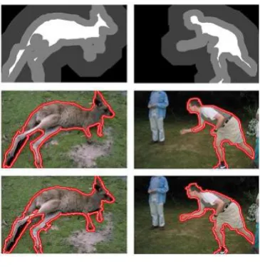
Fig (Top) Provided trimaps. (Middle) Results from random walks.(Bottom) Results using the proposed network.It can be seen that our proposed network successfully segments out the objects even when there are no enough labels atseveral critical components.The insufficiency in seeds is appreciable in the above two images , and our proposed method has worked well to address this problem.
VII. CONCLUSION
The task of segmenting semantically meaningful whole objects from images is a challenging issue. In the existing system, interactive image segmentation is done using Dirichlet Process Multiple-View Learning, but in this, classification accuracy is low for inefficient seeds and it takes high time complexity. With Dirichlet process mixture-based nonlinear classification, it can simultaneously model image features and discriminates between the object and the background classes In the proposed system, we are introducing Dynamic Bayesian Network in addition to Dirichlet Process – Multiple view learning. With the proposed learning, our segmentation framework is experimentally shown to produce both quantitatively and qualitatively promising results on a standard dataset of images. In particular, our proposed framework is able to segment whole objects from images given insufficient seeds.
REFERENCES
1. M.Andereetto,L.Zelnik-Manor and P.Perona,”Non-parametric probabilistic image segmentation” in Proc IEEE Int.Conf.Comput.Vis.,2007. 2. P.Arbelaez and L.Cohen,”Constrained image segmentation from hierarchical boundaries,” in Proc IEEE Int.Conf.Comput.Vis.,2008 3. P.Arbelaez,M.Maire,C.Fowlkes and J.Malik,”From contours to regions:An empirical evaluation,” in Proc IEEE Int.Conf.Comput.Vis.,2009 4. D.Blackwell and J.B.MacQueen,”Ferguson distributions via polyaurn scheme,” Ann.Stat.,vol 1,no.2,pp. 353-355,Mar 1973.
5. Y.Y.Bolycov and M.P.Jolly,” Interactive graph cuts for optimal boundary and regional segmentation of objects in n-d images,” in Proc IEEE Int.Conf.Comput.Vis.,2007
6. C.C. Chang and C.J. Lin,LIBSVM: A library for support vector machines 2001,Software.
8. L. Ding and A. Yilmaz, “Image segmentation as learning on hypergraphs,” in Proc IEEE Int.Conf.Comput.Vis.,2008
9. L. Ding and A. Yilmaz, “ Enhancing Intercative Image segmentation as using probablistc hypergraphs,” in Proc IEEE Int.Conf.Comput.Vis.,2010
10. L. Ding and A. Yilmaz, “ Interactive Image segmentation as learning on hypergraphs,” in Proc IEEE Int.Conf.Comput.Vis.,may 2010. 11. O. Duchenne, J. Y .Audibert,R. Keriven,J. Ponce and F.Segonne,”Segmentation By transduction” in Proc.IEEE .Conf.Comput.Vis.Pattern
Recog.,2008
12. A.A Ghorbani and K.Owarangh,”Stacked generalization in neural networks:Generalization on statistically neural problems,” in Proc.IEEE .Conf.Comput.Vis.Pattern Recog.,2008
13. L.Grady,”Random walks for image segmentation,”IEEE Trans.Pattern Anal .Mach.Intell,vol.28,Nov 2006
14. Y.D.Jain and C.S Chen,”Two-view motion segmentation with model selection and outlier removal by ransac-enhanced Dirichlet process mixture models,” Int.J.Comput Vis.,vol. 88,no.3,pp. 489-501,jul.2010.
15. K.Kurihara,M Welling, and Y.W.Teh,,”Collapsed vaiational Dirichlet process mixture models,” in Proc.Int.Joint Conf.Artif.Intell.,2007. 16. D.Larlus and F.Jurie,”Latent mixture vocabularies for object categorization and segmentation,” Image Vis.Comput.,vol.27,no.5,Apr.2009. 17. V.Lempitsky.P.Kohli,C.Rother,and T.Sharp,”Image segmentation with a boundary box prior,” in Proc.IEEE .Conf.Comput.Vis.Pattern
Recog.,2009