Wideband Direction of Arrival Estimation Based on the Principal Angle Between Subspaces

Wideband Direction of Arrival Estimation Based on the Principal

Angle between Subspaces

Zhiyu Feng1, Hongshu Liao2, *, Lu Gan2, Dong Yang2, and Rong Hu3

Abstract—In this paper, we propose a novel method for wideband direction of arrival (DOA) estimation. By calculating the largest principal angle between the signal subspace and the subspace spanned by the augmented array manifold, the proposed method can estimate direction of arrival of wideband signals. Unlike conventional wideband methods, it adopts a new augmented array manifold and constructs the augmented matrix entirely by processing the received signals in frequency domain. It does not require any preliminary DOA estimates or focusing matrices. Simulation results show that the proposed method exhibits satisfactory performance at medium and high signal-to-noise ratio (SNR) conditions in comparison to the existing wideband DOA estimation methods.

1. INTRODUCTION

Due to the increased use of wideband signals in the fields of wireless communication system and radar, the problem of direction of arrival (DOA) estimation of wideband signals has been of considerable interest to the array signal processing in recent years [1].

Quite a lot of algorithms have been proposed to estimate the DOAs of wideband signals, among which maximum-likelihood (ML) methods and subspace methods are the most well studied. The ML estimators show excellent performance, but multidimensional non-linear global search is needed [2]. The subspace methods, although not optimal, are more computationally attractive than ML methods. Subspace methods can be divided into two classes: incoherent signal subspace method (ISSM) and coherent signal subspace method (CSSM). Generally, ISSM [3] decomposes the array output into several narrow frequency portions and an individual processing is performed to estimate the DOAs of the signals at each frequency bin. Then a result is constructed by taking an average of DOAs at different frequency bins. While ISSM works well at high SNR, the performance degrades greatly when the SNR is low or varies at different frequency bins since even a single outlier from one frequency bin can potentially lead to inaccurate estimates through the averaging processing. ISSM can not handle coherent sources as well. To overcome these problems, several CSSM methods have been proposed [4–6]. These methods transform the correlation matrices at each frequency bin into one general correlation matrix at the focusing frequency by applying the focusing matrices. However, CSSM is sensitive to the focusing angles which are the initial estimates of the true DOAs [6]. In order to eliminate the preliminary DOA estimates’ influence, several improved methods were proposed such as the weighted average of signal subspaces (WAVES) [7] and the autofocusing CSSM [8]. Although WAVES and autofocusing CSSM methods can avoid initial estimates, their estimation performance could either not be held at high SNR or be likely to depend on the choice of the focusing frequency. A novel wideband DOA algorithm called test of orthogonality of projected subspaces (TOPS) [9] has been proposed. It is in between the coherent

Received 4 June 2018, Accepted 1 August 2018, Scheduled 23 August 2018 * Corresponding author: Hongshu Liao (shally [email protected]).

and incoherent processing and does not require initial estimates. However, the spatial spectrum of TOPS always shows spurious peaks which can potentially lead to false DOA especially when the number of the sources increases. A low rank signal model method was then proposed which can avoid preliminary DOA estimates and frequency domain processes, but it requires that the wideband signals should be n times differentiable, oversampled considerably for B-spline function approximation [10]. Yan presented a real-valued root MUSIC algorithm which exploits a subspace decomposition on the real-part of array covariance matrix [11, 12]. It can reduce the computational cost through sacrificing the sum number of estimating signal. Huang proposed a real-valued approach for wideband DOA estimation [13]. This method could enhance the resolution of angles while maintain a low calculation complexity. However, it only works well for spherical arrays. A wideband DOA estimation technique based on the A-shaped array for underwater passive target was presented [14]. The joint use of Bayesian learning model and expectation-maximization (EM) method in frequency domain was proposed to solve wideband DOA estimation, but it may increase the amount of computational complexity [15].

In this paper, we propose a new method of incoherent wideband DOA estimation based on the largest principal angle (LPA) [16] between two subspaces. Unlike the coherent methods which must align the signal and noise subspaces to form a general covariance matrix, this method only uses the LPA between the signal subspace and the subspace spanned by the augmented array manifold which contains all frequency bins for estimating the DOAs of the wideband sources. Simulation results indicate that the proposed method performs well at medium and high SNR conditions.

2. PROPOSED METHOD

Consider anM element linear array with unambiguous array manifold, and there areK(≤M) wideband incoherent sources s1(t), s2(t), . . . , sK(t) impinging on the array from different directions of arrival

θ1, θ2, . . . , θK respectively. The signal received at them-th sensor is given by

ym(t) =

K

k=1

sk(t−τm(θ_k)) +w_m(t), m= 0, . . . , M −1, (1)

where τ_m(θ_k) is the propagation delay associated with thek-th source at the m-th sensor, and w_m(t) is the additive noise at the m-th sensor. We sample the incoming signal at the frequency f_s and the entire samples are then partitioned into segments with P = ΔT f_s samples each. Then aP-point DFT is applied to theP samples in each segment. The DFT coefficients from the M sensors can be written as

Y(f_i) =A_θ(f_i)S(f_i) +W(f_i), i= 0,1, . . . , P −1, (2) where Y(f_i) = [Y1(fi)Y2(fi) . . . YM(fi)]T is an M ×1 vector with Ym(fi) being the DFT coefficient

of samples of x_m(t) at frequency f_i with f_i = _Pif_s. A_θ(f_i) = [a_θ1(f_i)a_θ2(f_i) . . .a_θK(f_i)] is an M×K matrix with a_θk(f_i) = [e−j2πfiτ1(θk)e−j2πfiτ2(θk) . . . e−j2πfiτM(θk)]T being the steering vector of the array at frequency f_i for the k-th source, and W(f_i) = [W1(fi) W2(fi) . . .WM(fi)]T and S(f_i) = [S1(fi) S2(fi) . . .SK(fi)]T are two vectors withWm(fi) andSk(fi) being the DFT coefficients at

frequencyf_i of the samples of w_m(t) and s_k(t), respectively. The operator (•)T denotes the transpose. We assume that ΔT is long enough compared to the correlation time of the signals and the noise. Therefore, the DFT coefficients can be regarded as uncorrelated.

Suppose that there are L segments with P samples of each. We calculate the DFT coefficients of each segment, pick outN frequency bins which vary fromf1 tofN, and then stack the DFT coefficients

of the same segment in sequence to form a column vector. We arrange the Lstacked column vectors in sequence to form anMN ×Laugmented data matrixYin frequency domain. Then it can be expressed by

A_θS+W =Y (3)

S=

⎡ ⎢ ⎢ ⎢ ⎣

S1(f1) S2(f1) · · · SL(f1) S1(f2) S2(f2) · · · SL(f2)

..

. ... . .. ...

S1(f_N) S2(f_N) · · · SL(f_N)

W =

⎡ ⎢ ⎢ ⎢ ⎣

W1(f1) W2(f1) · · · WL(f1) W1(f2) W2(f2) · · · WL(f2)

..

. ... . . . ...

W1(f_N) W2(f_N) · · · WL(f_N)

⎤ ⎥ ⎥ ⎥ ⎦

Y =

⎡ ⎢ ⎢ ⎢ ⎣

Y1(f1) Y2(f1) · · · YL(f1) Y1(f2) Y2(f2) · · · YL(f2)

..

. ... . . . ...

Y1(f_N) Y2(f_N) · · · YL(f_N)

⎤ ⎥ ⎥ ⎥ ⎦

where Sl(f_i) = [Sl₁(f_i) Sl₂(f_i) . . .Sl_K(f_i)]T represents the DFT coefficients of the l-th segment of the wideband sources at frequency f_i. Similarly, Wl(f_i) = [Wl₁(f_i) Wl₂(f_i). . . Wl_M(f_i)]T represents the DFT coefficients of the l-th segment of the additive noise at frequency f_i, and Yl(f_i) = [Yl₁(f_i) Yl₂(f_i) . . . Yl_M(f_i)]T are the DFT coefficients of the l-th segment of the receive signals at frequencyf_i. The matrixA_θ = blkdiag{A_θ(f1),Aθ(f2), . . . , Aθ(fN)}is an MN×NK block diagonal

matrix, where the symbol blkdiag{A_θ(f1),A_θ(f2), . . . , A_θ(fN)}represents a block diagonal matrix with

diagonal elementsA_θ(f1),A_θ(f2), . . . ,A_θ(fN). The following equations will be held on the assumption

that the additive white noise on each sensor is both spatially and temporally uncorrelated. E{wm(t)wm(t+τ)}= 0, τ = 0

E{wp(t)wq(t)}= 0, p=q (4)

Therefore, the sequence obtained from the DFT of the additive white noise remains white both in the frequency and space domain.

It is noted that the matrix A_θ is full rank with rank(A_θ) = NK. Since the columns of A_θ are independent, the finite-dimensional subspace spanned by the columns of A_θ is equivalent to the range of A_θ. It can be expressed as

R(A_θ) = ⊕N

j=1span

A_θ(f_j)

, (5)

where R(A_θ) denotes the range subspace of matrix A_θ. The operator ‘⊕’ denotes the direct-sum operator between subspaces. A_θ(f_j) is defined as following

A_θ(f_j) =

⎡

⎣ 0MA(j_θ−(f1)_j×)K

0_M(N−j)×K ⎤

⎦ _j = 1,2, . . . , N. (6)

From Eq. (3), the economy SVD of a noise-corruptedY can be expressed as following

Y =UΣVH, (7)

where U is an MN ×MN unitary matrix composed of left singular vectors {u_i, i= 1,2, . . . , MN}, and V is an MN × L unitary matrix composed of right singular vectors {v_i, i= 1,2, . . . , MN},

Σ= Diag(σ1, σ2, . . . , σMN) (σ1 ≥σ2· · · ≥σMN) is a diagonal matrix with real positive diagonal entries

called singular values of the matrix Y and the operator (•)H denotes conjugated transpose. Then, Y

can be expressed as

Y=σ1u1vH1 +σ2u2vH2 +· · ·+σNKuNKvHNK+σNK+1uNK+1vH_NK+1+· · ·+σMNuMNvHMN. (8)

We can divide the singular values of the matrixY into two parts. One contains theσ1,· · · , σNK,

which represents the signals plus noise, the other contains the σ_NK+1,· · · , σMN which only represents

noise. In practical application, we can determine the dimension of the signal subspace is NK via AIC or MDL [17] methods.

Then we have

Y= [U1U2]

Σ1 0

0 Σ2

whereU1 is anMN×NK unitary matrix composed by left singular vectors associated withNK bigger

singular values, andU2 is anMN×(MN−NK) unitary matrix composed by the rest of left singular

values. Then the subspaceU1 is the estimated signal subspace.

Considering that the number of sources is less than the number of sensor, then U1 has more rows

than columns. And

span(U1) = N

⊕

j=1span

A_θ(f_j)

, (10)

then we rearrange the columnsA_θ according to the directions of the sources. It can be expressed as

A_θ =

Ab_θ1 Ab_θ2 · · · Ab_θK

M_NK, (11)

whereAb_θk = blkdiag{a_θk(f1)a_θk(f2) · · ·a_θk(fN)}MN×N andMNK is aNK×NK permutation matrix.

Clearly, the augmented array manifold satisfies

span{Ab_θk} ⊂ N⊕ j=1

span{A_θ(f_j)}= span(U1) k= 1,2, . . . , K. (12)

Now for any θ, we can calculate the LPA which measures the “distance” between two subspaces which are the true signal subspace (given by the span of the columns of the augmented array manifold

Ab_θ) and the estimated signal subspace obtained through SVD of augmented data matrixY. The LPA between two matrices can be computed through

LPA(U1,U2) = cos−1

σmin

orth(U1)H·orth(U2)H

(13)

where orth(U_i)H,i= 1,2, is an orthonormal basis for the linear vector space spanned by the columns of U_i, and σmin(Z) denotes the smallest singular value of the matrix Z. The LPA is usually given in

degrees.

Particularly, LPA(Ab_θ,U1) = 0 will hold when span{Aθ} ⊂span(U1). It means that LPA(Ab_θ,U1)

will be 0 on the assumption that the scanning direction θ equals to one of the DOAs, otherwise, LPA(Ab_θ,U1) will be bigger than 0. Therefore we can find the source locations {θk}K_k=1 by finding the

minimum of angular spectrum.

The following steps summarize this proposed method of DOA estimation of wideband sources.

1) Compute the temporal DFT of the L data segments of received signal. 2) Arrange augmented data matrix Y according to Eq. (3).

3) Compute the economy SVD of Y and estimate the signal subspace U1.

4) Calculate LPA between the signal subspace U1 and the subspace spanned by the augmented array

manifoldAb_θ at different scanning direction.

5) Estimate the DOAs by finding the K minimum principal angles.

Remark: It is noted that the focusing process is avoidable because the augmented array manifoldAb_θ

contains all the frequency bins. The proposed method is similar to spectral MUSIC which is applicable to any array configuration [1, P. 1158]. Similarly, any arbitrary array geometry has its own augmented array manifold which is needed to calculate the LPA respectively.

3. SIMULATION AND ANALYSIS

We compare the performance of the proposed algorithm with those of the most widely used methods such as ML [2], ISSM [3], RSS [4], autofocusing CSSM [8] and TOPS [9]. Suppose that there are 3 wideband (i.e., K = 3) incoherent sources impinging on a 8 element uniform linear array (ULA) from 10◦, 20◦ and 30◦. The sources cover the frequency band between 0.6π and π in the digital frequency domain. The sensor spacing is chosen to be λ0/2 where λ0 is the wavelength corresponding to the

The samples of impinging signal are divided intoL = 100 segments of P = 256 samples each. In each segment the 256 samples are converted to frequency domain by a 256-point DFT, which are then processed using six different algorithms: a) the proposed method. b) ISSM method. c) CSSM using RSS focusing matrices with initial DOA estimates [8◦,18◦,32◦]. d) Autofocuing CSSM method. e) The TOPS algorithm. f) the maximum-likelihood method. All The focusing matrices are constructed following [4] and the focusing frequency is chosen to be the lowest frequency of the band. It is to be noted that only ten frequency bins (i.e., N = 10) are used in the proposed method and all the conventional methods. 500 independent Monte Carlo trials have been carried out for each simulation.

Simulation test 1: performances of the six algorithms are compared for the source at 20◦ in terms of their root-mean-squared error (RMSE) in Fig. 1(a) (here, we suppose that there is only one signal impinging on the array from 20◦ and the initial DOA are [18◦] for the RSS algorithm). As expected,

0 5 10 15

0 0.02 0.04 0.06 0.08 0.1 0.12 0.14 0.16 0.18 0.2 RMSE (degree) Proposed ISSM Autofocus Rss TOPS ML

-600 -40 -20 0 20 40 60 10 20 30 40 50 60 70 80 90

scanning angle (degree)

LPA-spectrum (degree) SNR=-10dB SNR=0dB SNR=10dB SNR=20dB SNR=30dB

10 15 20 25 30 0 5 10 15 (a) (b) SNR (dB)

Figure 1. (a) Comparison of RMSE of the different wideband DOA estimation algorithms v/s SNR for single source at 20◦. (b) Comparison of LPA-spectrums of the proposed algorithm under different SNR. 0 0.1 0.2 0.3 0.4 0.5 0.6 0.7 0.8 0.9 1 pseudo-spectrum True DOA

The pseudo spectrum of TOPS

0 10 20 30 40 50 60 70 80 90 LPA-spectrum (degree) True DOA

The LPA spectrum of the proposed method

(a) (b)

-60 -40 -20 0 20 40 60

scanning angle (degree)

-60 -40 -20 0 20 40 60

scanning angle (degree)

the ML method performs best among the six methods. The performance of the proposed method is less than the ML’s and TOPS’. The RSS suffers even at high SNR due to the poor initial DOAs (in fact, the initial DOA in our experiment is less than 2◦), the ISSM and autofocusing method perform worse than the proposed method when SNR is larger than 2.5 dB.

Simulation test 2: suppose that there are 3 wideband signals impinging on the ULA, and the simulation condition is the same as the Simulation test 1. The comparison of LPA-spectrums of the proposed method under different SNRs is shown in Fig. 1(b). It is clear that with the increase of SNR, the LPA-spectrum peaks show better sharpness, and there are almost no false peaks when SNR is larger than 0 dB.

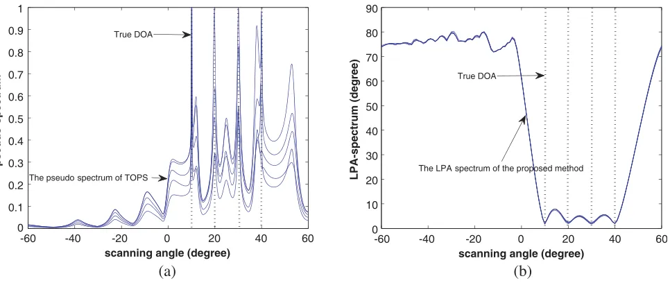
Simulation test 3: suppose that another signal is impinging at 40◦ besides the 3 wideband signals as shown in simulation test 2. Figs. 2(a), (b) show the pseudo-spectrums of the TOPS and the LPA-spectrums of the proposed method for 5 trials when SNR = 15 dB and snapshots = 100, respectively. It is shown that the pseudo-spectrums of the TOPS have spurious peaks but it would not occur in LPA-spectrums of the proposed method. With the increase of the number of sources, the spurious peaks will suffer more in TOPS method.

4. CONCLUSIONS

In this paper, we have proposed a new wideband DOA estimation algorithm based on the largest principal angle between subspaces. The proposed method adopts a new array manifold containing all the frequency without focusing process and is applicable to any array geometry. It provides a solution to avoiding the requirement of initial DOA estimates, while exhibiting the desirable performances better than the coherent methods. It can overcome the drawbacks of the TOPS method without spurious peaks. Simulation results show that it exhibits a satisfactory performance at medium and high SNR.

ACKNOWLEDGMENT

This work was supported by the Technology Research Project of Chongqing Municipal Education Commission of China (KJ1602201).

REFERENCES

1. Van Trees, H. L., Optimum Array Processing: Part IV of Detection, Estimation and Modulation Theory, Vol. 1, Wiley Online Library, 2002.

2. Doron, M. A., A. J. Weiss, and H. Messer, “Maximum-likelihood direction finding of wide-band sources,”IEEE Transactions on Signal Processing, Vol. 41, No. 1, 411, 1993.

3. Wax, M., T.-J. Shan, and T. Kailath, “Spatio-temporal spectral analysis by eigenstructure methods,”IEEE Transactions on Acoustics, Speech, and Signal Processing, Vol. 32, No. 4, 817–827, 1984.

4. Wang, H. and M. Kaveh, “Coherent signal-subspace processing for the detection and estimation of angles of arrival of multiple wide-band sources,” IEEE Transactions on Acoustics, Speech, and Signal Processing, Vol. 33, No. 4, 823–831, 1985.

5. Valaee, S. and P. Kabal, “Wideband array processing using a two-sided correlation transformation,” IEEE Transactions on Signal Processing, Vol. 43, No. 1, 160–172, 1995.

6. Swingler, D. N. and J. Krolik, “Source location bias in the coherently focused high-resolution broad-band beamformer,”IEEE Transactions on Acoustics, Speech, and Signal Processing, Vol. 37, No. 1, 143–145, 1989.

7. Di Claudio, E. D. and R. Parisi, “Waves: Weighted average of signal subspaces for robust wideband direction finding,” IEEE Transactions on Signal Processing, Vol. 49, No. 10, 2179–2191, 2001. 8. Pal, P. and P. Vaidyanathan, “A novel autofocusing approach for estimating directions-of-arrival

9. Yoon, Y.-S., L. M. Kaplan, and J. H. McClellan, “Tops: New DOA estimator for wideband signals,” IEEE Transactions on Signal Processing, Vol. 54, No. 6, 1977–1989, 2006.

10. Mahata, K., “A subspace algorithm for wideband source localization without narrowband filtering,” IEEE Transactions on Signal Processing, Vol. 59, No. 7, 3470–3475, 2011.

11. Yan, F.-G., M. Jin, S. Liu, and X.-L. Qiao, “Real-valued music for efficient direction estimation with arbitrary array geometries,” IEEE Transactions on Signal Processing, Vol. 62, 1548–1560, 2014.

12. Yan, F.-G., Y. Shen, and M. Jin, “Fast doa estimation based on a split subspace decomposition on the array covariance matrix,”Signal Processing, Vol. 115, 1–8, 2015.

13. Huang, J., Q. Huang, L. Zhang, and Y. Fang, “A real-valued approach for wideband DOA estimation using spherical arrays,”Signal Processing, Vol. 125, No. C, 79–86, 2016.

14. Shi, J., Q. F. Zhang, and Y. Wang, “Wideband DOA estimation based on A-shaped array,” IEEE International Conference on Signal Processing, Communications and Computing (ICSPCC), 1–5, 2017.

15. Hu, N., B. Sun, J. J. Wang, and J. F. Yang, “Covariance-based DOA estimation for wideband signals using joint sparse Bayesian learning,”IEEE International Conference on Signal Processing, Communications and Computing (ICSPCC), 1–5, 2017.

16. Golub, G. H. and C. F. van Loan,Matrix Computations, 374–426, Johns Hopkins University Press, Baltimore, MD, USA, 1996.