University of Windsor University of Windsor
Scholarship at UWindsor
Scholarship at UWindsor
Electronic Theses and Dissertations Theses, Dissertations, and Major Papers
1-1-2007
The extensible runtime infrastructure for particle simulations with
The extensible runtime infrastructure for particle simulations with
data-space management and adaptive resource allocation.
data-space management and adaptive resource allocation.
Yu Zou
University of Windsor
Follow this and additional works at: https://scholar.uwindsor.ca/etd
Recommended Citation Recommended Citation
Zou, Yu, "The extensible runtime infrastructure for particle simulations with data-space management and adaptive resource allocation." (2007). Electronic Theses and Dissertations. 7010.
https://scholar.uwindsor.ca/etd/7010
The
Extensible
Runtime
Infrastructure
for
Particle
Simulations with Data-Space Management and Adaptive
Resource Allocation
by
Yu Zou
A Thesis
Submitted to the Faculty o f Graduate Studies
through C om puter Science
in Partial Fulfillm ent o f the Requirem ents for
the Degree o f M aster o f Science at the
U niversity o f W indsor
Windsor, Ontario, Canada
2007
Library and Archives Canada
Bibliotheque et Archives Canada
Published Heritage Branch
395 W ellington Street Ottawa ON K1A 0N4 Canada
Your file Votre reference ISBN: 978-0-494-35037-9 Our file Notre reference ISBN: 978-0-494-35037-9
Direction du
Patrimoine de I'edition 395, rue W ellington Ottawa ON K1A 0N4 Canada
NOTICE:
The author has granted a non exclusive license allowing Library and Archives Canada to reproduce, publish, archive, preserve, conserve, communicate to the public by
telecommunication or on the Internet, loan, distribute and sell theses
worldwide, for commercial or non commercial purposes, in microform, paper, electronic and/or any other formats.
AVIS:
L'auteur a accorde une licence non exclusive permettant a la Bibliotheque et Archives Canada de reproduire, publier, archiver,
sauvegarder, conserver, transmettre au public par telecommunication ou par I'lnternet, preter, distribuer et vendre des theses partout dans le monde, a des fins commerciales ou autres, sur support microforme, papier, electronique et/ou autres formats.
The author retains copyright ownership and moral rights in this thesis. Neither the thesis nor substantial extracts from it may be printed or otherwise reproduced without the author's permission.
L'auteur conserve la propriete du droit d'auteur et des droits moraux qui protege cette these. Ni la these ni des extraits substantiels de celle-ci ne doivent etre imprimes ou autrement reproduits sans son autorisation.
In compliance with the Canadian Privacy Act some supporting forms may have been removed from this thesis.
While these forms may be included in the document page count,
their removal does not represent any loss of content from the
Conformement a la loi canadienne sur la protection de la vie privee, quelques formulaires secondaires ont ete enleves de cette these.
Abstract
Running an adaptive particle simulation on a distributed parallel environment is a
challenge, which requires dynamically periodic repartitioning during the course of
computation. Repartitioning is also necessary under time and space adaptive resource
allocation. This thesis presents an implementation of dynamic and adaptive resource
management middleware for scientific particle simulation problems. We optimized
ATOP [20] data structure to greatly reduce the total data migration time and support data
cache locality. In addition, a simplified interface is designed for typical particle
simulation problems, which makes the library more useable for general scientific
computation. The thesis presents the implementation of an initial solution and the design
of a further optimized solution for future extension.
The library had been tested on a distributed memory cluster machine with typical
bench mark simulation data graphs; and experiment results show that our optimized data
structure decrease mesh adaptation time 55-99% and memory management can reduce
Dedication
To
My wife, my daughter
and
Acknowledgement
I would like to acknowledge my gratefulness to Dr. A.C. Sodan fo r her supervision during
this thesis work. Without her guidance and help, it would not be possible fo r me to finish
this work. I also thank Lin Han fo r his work on ATOP which provides a start point fo r my
work. I appreciate my committee members: Dr. Dan Wu, Dr. Wai Ling Yee and Dr.
Xianbu Yuan, who have been kind and patient during the time when I present my thesis
work.
Finally, I thank my family, my wife and my lovely daughter, fo r their consistent support
Table of Content
1. Introduction...1
2. P a rtic le S im u la tio n s... 4
2.1 Typical Particle Simulation Phases...5
2.2 Cost Model... 7
3. P a rtitio n in g A lg o rith m s a n d A d a p tiv e R e so u rc e A llo c a tio n ...9
3.1 Partitioning Algorithms...9
3.2 Work Load Distribution Algorithms... 10
3.3 Zoltan Partitioning and Load Balance Library... 11
3.4 Adaptive Resource Allocation Systems... 12
4. D a ta L o c a lity M a n a g e m e n t... 14
5. O u r A p p r o a c h ... 17
5.1 Basic Concepts...17
5.2 Architecture of the Runtime Library System... 18
5.3 Internal Data Structures... 20
5.3.1 Mesh Data Structure... 21
5.3.2 Partition Structure... 23
5.3.3 Node Structure... 24
5.3.4 Borders and Ghosts... 27
5.4 Interfaces... 29
6
Experim ents and R esults
...346.1 Experim ent Environm ent...34
6.2 Adaptation Performance...35
6.2.1 Adaptation Experiments in a Space-shared Environment... 35
6.2.2 Adaptation Experiments in a Time-shared Environment...40
6.3 Data Locality Management Module Performance Experiments... 42
6.3.1 Computation Time in Static Environment... 43
6.3.2 Computation Time in Dynamic Environment... 45
6.4 Experim ent Sum m ary...47
7 Further Possible Im provem ents... 49
7.1 Optimized Data Structure... 49
7.2 Adding Memory Management... 50
7.2.1 Block Level Management... 51
7.2.2 Node Level Management... 53
7.3 Latency Hiding by Asynchronous Communication...55
APPENDIX
A
B ibliography...
59B
D ata Structures...
63C
Sample A pplication...
67D
ATOP_M ESH_CM M PUTE()...
70List of Tables
Table 1. Benchmark Graphs...34
Table 2. Adaptation by over partitioning in space-shared environment with 8 partitions...36
Table3. Adaptation by partitioning from scratch in space-shared environment with 8 partitions...37
Table 4. Init time and adaptation time by over-partitioning for 16 partitions...38
Table 5. Init time and adaptation time by partitioning from scratch for 6 partitions...38
Table 6. Init time and adaptation time by over-partitioning with 128 partitions... 38
Table 7. Init time and adaptation time by ATOP environment with 128 partitions... 41
Table 8. Init time and adaptation time by K-way Partitioning from scratch with 128 partition...41
Table 9. Computation time in a static environment...43
List of Figures
Figure 1. Typical Simulation Phases...6
Figure 2. 2D Structured Mesh with 4 Partitions...6
Figure 3. Simulation Phases in Shared Environment...13
Figure 4. System Architecture... 18
Figure 5. System Class Diagram... 19
Figure 6. Local information 1...22
Figure 7. Local information 2 ...23
Figure 8. Aligned Normal Nodes...25
Figure 9. Aligned Nodes Bordered to One Processor... 26
Figure 10. Aligned Nodes Bordered to Multiple Processors... 26
Figure 11. Border List Structure... 28
Figure 12. Ghost Nodes... 29
Figure 13. Interfaces...31
Figure 14. Un-aligned Partitions...32
Figure 15. Aligned partitions... 33
Figure 16. Comparison for 16 partitions by ATOP... 39
Figure 17. Comparison for 16 partitions by partitioning from scratch... 39
Figure 18. Comparison for 128 partitions by ATOP...40
Figure 19. Computation time charts in a static environment... 44
Figure 20. Optimized Class Diagram... 50
Figure 22. Linked List of Block before Allocation... 52
Figure 23. Linked List of Block after Allocation...52
Figure 24. Before free block A ... 53
Figure 25. After free block A ... 53
Figure 26. Internal Block Structure...54
Figure 27. Blocks for Different-sized Nodes...54
1
Introduction
Particle simulation is used for the dynamic representation of a wide range of
natural phenomena such as Computation Fluid Dynamics (CFD) and Computational
Electro Magnetics (CEM) and so on. Because of the big amount of data for the class of
problems, which can be millions of nodes in one mesh, simulations of these problems
usually need be executed on NUMA machines [7], like clusters or on a grid in order to
overcome the physical limitation of processing capability. These scientific simulations
also require that periodic repartitioning happens dynamically throughout the computation
course. The repartitions must be computed to minimize both the inter-processor
communication cost incurred during the iterative mesh-based computation and the data
redistribution costs required to balance the load. However repartitioning and re
distributing data for scaled problems can also be very expensive, and the situation
becomes even worse when the simulations are executed in a time-shared and space-
shared environment. So a good adaptive resource allocation runtime approach is critical
to reach a high throughput and better utilization of resources.
ATOP [20] provides an effective approach to solve the problem. First, it uses
over-partitioning (pre-partitioning) of data at the very beginning or when it is necessary.
When unbalanced load happens during a computation process, the system can be re
balanced by directly distributing current partitions among available nodes other than
repartitioning data from scratch. Second, ATOP always uses as many processes as
space shared and time shared resource management. However, ATOP was not yet a
fully-fledged middle-ware system: It does not allow dynamically switch between space-
shared and time-shared adaptation; and it also requires searching to access to each node
which adds huge overhead during migration phase. All of these weaknesses will be fully
overcome in our new middleware system by applying new system design and
implementation.
A good load balance algorithm balances work load among processors in a
distributed environment, and keeps as few edge-cuts as possible among
partitions/processors in order to avoid unnecessary communication among
processors[6][9]. This can be considered as data locality management mechanism at
distributed memory level by trying to keep data in local memory. On the other hand, data
locality in a NUMA system can also be managed at cache level. We implement our data
cache locality management by putting each partition data into a continuous aligned
memory block and making each block fit into the cache of local processors, which
reduces cache misses during the computation process. Our test shows that using inline
partition data memory block can speed computation time up to 20%.
A desirable property of a run-time system is its ability of providing services with
transparency. Then users are able to use it without totally re-write their programs. The
interface provided in our project hides all implementation details and provides users a set
of simple functions for a specific application area, which also adds to our middleware
The structure of this thesis is arranged the following way: In Chapter 2, we will
review particle simulations and dynamic resource allocation; Chapter 3 will cover data
locality management, and Chapter 4 focuses on our approach; and finally experiment and
result are to be discussed in Chapter 5. Chapter 6 will show future possible optimizations
2
Particle Simulations
A particle system usually refers to a computer technique to simulate various
natural and scientific processes, which are difficult to reproduce with traditional
rendering techniques. Examples of such phenomena which are commonly done with
particle systems include fire, explosions, smoke, flowing water, sparks, falling leaves,
clouds, fog, snow, dust, meteor tails, etc.
Typically, particles are objects that have mass, position, velocity, and respond to
forces, but have no spatial extent. A typical particle data structure from users’ view may
look like:
typedef structf
float m; /* mass */
float *x; /* position vector * /
float *v; /* velocity vector */
float *f; /* force accumulator */
int *nbors /* Adjacent particle */ } * Par t i d e ;
Then for a whole particle system may look like:
typedef structf
Particle *p; /* array of pointers to particles */
int n; /* number of particles */
float t; /* simulation clock */
} *ParticleSystem;
Besides the particle data structure, a particle system also includes a solver, which
is a simulation function applied to the particle system. The solver may have interface like:
void Calculate (ParticleSystem, Particle);
Inside this function, the solver computes new values for each particle for the next
updated according to some computation functions for the specific simulation. For
example, the new position values for a particle P* can be expressed as a function of its
own mass, current position, current velocity, forces and its neighbor’s positions:
P* -> x [i] = / ( P*->m, P* -> x[i], P* ->v[i], P* -> nbor[i], P* -> f[i])
Similarly, new values of velocity for the particle can also be expressed as
functions of positions, velocity, and forces, etc.
P* -> v [i] = /(P*->m , P* -> x[i], P* ->v[i], P* -> f[i])
2.1
Typical Particle Simulation Phases
For large-scale scientific particle simulations, efficient execution on parallel
computers requires periodic repartitioning of the underlying computational mesh. This
repartitioning should minimize both the inter-processor communications incurred in the
iterative mesh-based computation and the data redistribution costs required to balance the
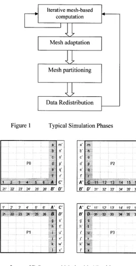
load. Figure 1 illustrates the typical steps involved in the execution of adaptive mesh-
based simulations on parallel computers. And Figure 2 shows a 2D structured mesh with
4 partitions. Initially, the data mesh is distributed among the processors according to a
specific load-balancing scheme. Then a number of iterations of a simulation computation
are performed in parallel. After that, either mesh adaptation happens as local processors
refine or redefine their local regions of mesh that leads to unbalanced work load among
processors in the whole system. Then re-partitioning based on the current mesh and
respectively. The simulation can then enter another simulation iteration phase until either
more unbalanced load happened or the simulation terminate.
Iterative mesh-based computation
1
s ✓7
Mesh adaptation
s ✓7
Mesh partitioning
\ ✓7
Data Redistribution
Figure 1 Typical Simulation Phases
m' a ’ m
b n' b' n
C o' c' c
: PO :d.. P' d' F P2
e q.' e' c
f r' f i
1 2 3 4 5 6 4 C ’ 4 ’ C 11 12 13 14 15 16
21' j 22' : 23' ; 24' 25' 26' I B ' O’ O ’ O' : 31' : 32' : 33' : 34' 35' ; 36'
1' 2' 5' 4' 5' 6' 4 ’ c A' C 11' : 12' ; 13' 14' 15' 16'
21 22 23 24 25 26 8 O ' 8' D 31 32 33 34 35 36
... ... g s' g' S
h t' h' t
; PI ; i u' r u i: ■P3 :
... ■ ,:j- v' j' V "“k"" w ' k' w
k' i' . X
2.2
Cost Model
Considering the general processing steps illustrated in the above figure, and each
round of executing includes a number of iterations of the simulation, a mesh adaptation,
and load-balancing which make repartitioning and redistribution, then every round of
executing will have the run time like:
Where n stands for the number of iterations for simulation computation, Tcmp is the run
time to perform the computation for a single of the simulation, Tcmu is the time caused by
the communication for a single iteration, and Trepar and T^st stand for the run time of
repartitioning and data redistribution respectively in a round [20].
Furthermore, communication time among processors depends on the number of
edge-cut of the partitioning if we ignore the speed of physical computer. This can be
expressed as a function of edge-cut:
On the other hand, data redistribution time can be described as a function of total amount
of data to be moved in order to rebuild the new balanced load among processors, then we
have:
n * (Temp + Tcmu) + Trepar + Tdist (1)
emu (2)
Tdist £ (V m o v )
(3)
Combine formulas (1), (2), (3) we get total run time:
Adaptive repartitioning affects all of the terms in above formula (4). The quality
of the new partitioning influences Tcmp. The number of edge-cuts of a new partitioning
affects the inter-processor communications time. The data redistribution time is
dependent on the total amount of data that is required to be moved in order to rebuild a
balanced load among processors.
Generally those current adaptive repartitioning schemes
[4][5] [12] [13] [14][15] [16] [17] [18] [21] [22] tend to be very fast and well balanced, which
are dependent on the partitioning algorithm. Computation time not only depends on the
simulation itself, it also depends on how efficient the runtime system can be. This is
usually related to system architecture, memory management and other implementation
details. From the perspective of partitioning and repartitioning, b o t h /(Ecut)) and g (Vmov)
can seriously affect parallel run times and drive down parallel efficiencies. Therefore, it
is critical for adaptive partitioning schemes to attempt to minimize both the edge-cut and
the data redistribution cost when computing the new partitioning. From this point,
3 Partitioning Algorithms and Adaptive Resource Allocation
3.1
Partitioning Algorithms
Since it is hard to have both/ (Ecut)) and g (Vmov) minimized, adaptive partitioning
algorithms can be classified into two categories: The first category is to focus on
minimizing the edge-cut and to minimize the data redistribution only as a secondary
objective [12][18] [22], They make the best effort to compute a new partitioning from
scratch and then attempt to intelligently remap the sub-domain labels to those of the
original partitioning in order to reduce the data redistribution costs. Some state-of-the-art
graph partitioners are used to compute the partitions, the resulting edge-cut tends to be
extremely good. However, since there is no guarantee to how similar the new partitioning
will be to the original partitioning, data redistribution costs can be high, even after
remapping. The second category is to focus on minimizing the data redistribution cost
and to minimize the edge-cut as a secondary objective [4][14][15][16][21], These
schemes attempt to perturb the original partitioning just enough so as to balance it. So
they usually lead to low data redistribution costs, especially when the partitioning is only
slightly imbalanced. However, it can result in higher edge-cuts than partitioning from
scratch methods because perturbing a partitioning in this way also tends to adversely
affect its quality.
ATOP [20] is more like an approach that combines those two categories. It first
over-partitions the whole graph and then during the load re-balancing phase it can
redistribute data without re-partitioning from the scratch. Meanwhile, it still provides the
their test result, ATOP shows a moderate increase of the number of edge cuts and it can
decrease adaptation time to 20%-30%.
3.2
W ork Load Distribution Algorithms
Partitioning is the first step of adaptive load balancing. After partitioning, data
needs to be distributed to corresponding processors. Depending on the location of the
load balancer, load balancing algorithms can be categorized as centralized or distributed.
If the load balancer is located in one processor, and it has global load information of all
nodes and can initiate the process of work load balancing, we call it a centralized load
balancing approach. On the other hand, if each node has a load balancer which can
broadcast load information to its neighbors or all other nodes, we call it a distributed load
balancing approach. Because there must be one master processor to take care of the
processing of load balancing, centralized approaches have limitations of scalability and
are more suitable for a small number of nodes [25]. Performance of centralized
approaches degrades along with the increased number of processors. Distributed
approaches can be more scalable, but since global load information spreads among nodes
and a node may only broadcast its load information to its neighbors, the whole system is
lacking a global load profile, making these approaches less efficient as centralized
approaches.
Depending on when the work load is redistributed to nodes, again load balancing
algorithms can be divided into synchronous and asynchronous. Synchronous load
balancing process. After partitioning and data redistribution each node resumes its other
work. Asynchronous load balancing doesn’t require that all nodes stop simultaneous for
load balancing. Usually it uses work-stealing algorithms to redistribute work among
nodes asynchronously, which then provides the advantage of latency hiding between
computation and adaptation [3], The disadvantage of this approach is that it also has
worse load balancing quality, compared to the synchronous one.
3.3
Zoltan Partitioning and Load Balance Library
Zoltan [2] is a portable library that provides set of load balance and partition tools
based on MPI. It can also run on different physical platforms. ATOP uses it as partitioner
and migration tool. This makes ATOP more useable for different environments.
Moreover, Zoltan supports a wide range of partitioning algorithm such as Recursive
Coordinate Bisection (RCB), Recursive Inertial Bisection (RIB), and incorporates with
JOSTLE and ParMETIS[10], ATOP uses both Zoltan and ParMETIS; this fits the
requirement that our system should be extensible when users need to tune it for their
special usages.
Zoltan does not have special requirements on structures of nodes and meshes.
However, users do have to provide global information and local information of the whole
mesh and individual nodes by setting up a series of call-back functions. For example,
users have to provide the total number of nodes of the whole mesh, global and local id of
each node, data packing and unpacking, neighboring information of each node and so on.
Somehow this is still inconvenient and time consuming for users. This is where our
3.4
Adaptive Resource Allocation Systems
Adaptive resource allocation can get better response time and resource utilization
in a time-shared and space-shared environment. Running a parallel application with
adaptive resource allocation also needs cooperation from the application, which has to be
malleable [22], i.e. the application needs to be adaptive to changes of available processors
during the runtime. ATOP’s main goal is to provide support to make simulations
malleable and able to run in a shared environment with adaptive resource allocation.
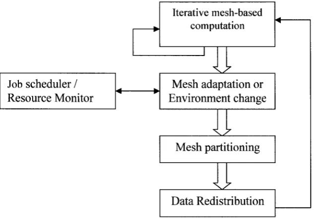
Adaptation for a simulation is actually a process of load balancing, which
typically needs two components: partitioner and load balancer. To make the process
adaptive to a time-shared and space-shared environment, two more components are
necessary: resource monitor and job scheduler. See Figure 2. So not only does adaptation
happen when it is needed from the simulation phases, it also happens when the runtime
environment changes. When the local workload changes like extra nodes being available
or new jobs having been scheduled on the system, the resource monitor or job scheduler
Iterative mesh-based computation
Mesh partitioning
Data Redistribution
Job scheduler / Mesh adaptation or
Resource Monitor Environment change
Figure 3 Simulation Phases in Shared Environment
On a NUMA system or a grid computer system, parallel execution of applications
is generally based on message passing. MPI (message passing interfaces) has become the
de facto parallel programming paradigm. However, so far only few runtime resource
allocation systems are built on message passing. TMPI [19] and Cilk [1] tried to use
threads to replace local MPI processes which are more suitable for running on a SMP
shared memory machine. AMPI [8] tried to use threads to over-partition into MPI
“process” and balance these threads to nodes according to load information. The major
problem with these thread-based systems is that a large number of threads per node tend
to result in a big thread context switch overhead, and slow down applications if
communication is frequent. However, scientific particle simulations are communication
intensive. After every round of mesh computation, communication for exchanging local
4
Data Locality Management
In the last decades, the speed of processor doubled for every 2-3 years but
memory access speed only improved 10% every year. The gap between CPU speed and
memory access speed has become a bottleneck for enhancing computing power. In order
to reduce this gap, modem computers resort to multilevel memory hierarchies. Usually
modem computers have two levels of cache memories, and further NUMA machines
have both local memory and remote memory, where local memory can be considered as
the cache of the remote memory. However, computing performance improvement with
this memory structure depends on whether the caches can provide data that an application
needs at runtime, because cache misses will result in spending extra time to access data
from higher-level memory. So application performance becomes very sensitive to the
cache hits.
For particle simulation applications, improving data locality of applications will
lead to better performance. From formula (4), data locality can affect all the factors of a
particle simulation, especially Tcmp and Tcmu because a typical particle simulation tends to
repeat hundreds and even thousands of times to compute mesh between two sequential
mesh adaptations, and total number of repeated computation for a whole simulation may
reach to millions. Bad data locality always slows down a simulation during running time.
Even a small amount of saving time during the computation phase can contribute a big
Data locality in a NUMA machine usually can be achieved at two levels. The
higher level or network level data locality can be provided between the local memory and
remote memory. Better partitioning strategies keep more needed data in local nodes, and
network latency and communication cost can be reduced. So, as we discussed in Chapter
2, those partitioning algorithms focus on minimizing edge-cuts among partitions [12] [22]
will have better data locality. In addition, this level of locality can be obtained by keeping
some extra data on local nodes: besides storing those vertices that belong to the local
mesh, all neighbor vertices will have a copy stored in local memory, which are called
ghost cells. For example, Figure 3 shows that four processors with local meshes. Shaded
cells are border nodes and labeled cells are ghost cells.
Cache locality can be provided at local processors only. On a time-shared
machine, there are two factors influence cache locality: 1), several processes or threads
share the same cache. One running process or thread displaces the cache content which
was built by the previous running process or thread. When the previous process or thread
runs again it will encounter a series of cache misses. 2), either memory fragmentations or
random memory accesses will affect utilization of cache lines. In time shared
environments we can not avoid processes or thread switches, but we still can obtain better
cache locality by optimizing application data structure. To achieve this goal, the order of
access to data is crucial. By sorting or aligning all local data in memory, all memory
access patterns for this problem can become sequential as opposed to random. This
allows maximum use of hardware-based performance features such as caching and
ignored for current adaptive runtime systems due to the implementation complexity and
5
Our Approach
Our objective is to implement an efficient dynamic resource allocation
middleware for scientific particle simulations. We reach this goal by finishing the
following jobs in our project:
• Extend ATOP partitioning and load balancing algorithm by using optimized data
structures to do direct accesses.
• Add data locality management to ATOP by aligning local data into blocks of
continuous memory to provide cache locality.
• Add communication management by using border-ghost mapping to
automatically communication and make communication more efficient by
aligning packing and unpacking.
• Implement switching between time-share adaptation and space-shared adaptation.
• Interface makes the middleware easy to use.
5.1
Basic Concept
Definition: Space Adaptation'. The number of processors allocated to an
application can be changeable dynamically during runtime [20],
Definition: Time Adaptation: The time share allocated to an application can be
different on different processors and can be changed dynamically during the application’s
5.2
Architecture of the Runtime Library System
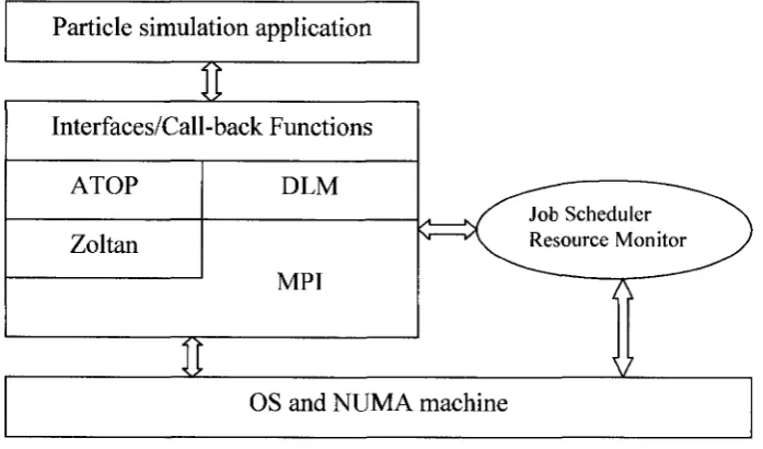
In our architecture, see Figure 4, the operating system is at the bottom and above
that the MPI library is located. The ATOP load balancing algorithm and our data locality
management (DLM) module lie above Zoltan and MPI, which manages memory
alignment, optimization, border cells and ghost cells. We use the ATOP algorithm to
over-partition the data mesh and handle dynamic adaptation when an adaptation is
necessary. We redesigned internal data structures of ATOP to avoid searching problems
and also make dynamic switching between time-shared and space-shared allocation
possible. Beneath ATOP and DLM is the Zoltan load balancing library which provides
multiple partitioning and data management tools.
Particle simulation application
3E
1
Interfaces/Call-back Functions
ATOP DLM
Zoltan
MPI
Job Scheduler Resource Monitor
T T
i z . OS and NUMA machine
Figure 4 System Architecture
The Interfaces and call-back functions layer is above ATOP and DLM, and
encapsulate all the implementation detail from the users and provide users simple and
from too much attention on dynamic variations in computational load and communication
patterns. So we provide a simplified set of interfaces in order to keep users from dealing
those tedious lower level works such as load balancing, data management, migration and
etc. Detailed interfaces will be discussed in Section 4 of this chapter.
—g lo b a l in fo — _ n o d e s : int + m a x _ n u m _ o f „ e d g e s : int + m a x _ r n j D _ o f .p a r t it io n s : int 4 -n u m _p roc: int + p a r j p r o c J d _ a r r : int* + partitiQ n_nun-i_arr: 'mt* + p r o c _ J d _ a r r: in t* — fo c a l in fo —; 4 - p r o c J d ; int 4-num _bf_Jocals: int + p a r _ n u m _ o f J o c a ls i Int + n o d e j J t r _ a r r : Nocle_Pfcr* 4 -p ar_p tr_arr: Partition_Pfcr — g h o s t in fo — 4 -g h o s t J is t ; P artftion_P tr
P a r ti tio n
+partition _riu m : int + p a rb tto n _ lo ca i_ ld : int + n u m _ o f _ n o d e s : int + le n g th _ n o d e _ id _ a r r : int* + n o d e _ p tr_arr: int* 4-isA ligned: int — b o rd er in fo — + n u m _ b o r e r J is t : int
+ b o r d e f J is t_ p tr _ a r r : B order_L ist*'
INode
+ gl< ± > aljd : int + lo c a l_ id : int + n u m _ a d j_ n o d e : int + id _ ln jja r t it io n : int + a d j _ n o d e _ a r r : int* + e d g e _ w g t _ a r r : flo a t* + c o m p u _ w g t: f lo a t* + s t a t u s _ f ia g : ch ar + n o d e „ d a t a ^ 3 t r : v o ld [2j
Border_List 4 -b o r d e r jD r o c J d : int 4 -n u m „ b o r d e r _ n o d e : int -+-global_td_arr: int* 4-list J e n g t h ; int 4 -b o r d e r _ d a ta _ p tr : c h a r * [ 2 ]
NodeJ>ata
Figure 5 System Class Diagram
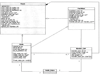
We use an objective-oriented technique to design and implement our system,
though we still use C as programming language for this project. The whole system is
illustrated as class diagram like Figure 5. From the diagram, we can see that the main
data structures are node, mesh and partition, node contains all necessary information
and related operations of a node such as global id, local id, number of adjacent nodes and
etc. mesh includes all the global and local information for a mesh. Technically a mesh is
All related operations / functions are defined in header files mesh.h, partition.h and
node.h. The public accessibilities for all data members and methods in the UML diagram
means they are accessible for C programming language as long as a right header file is
included.
5.3
Internal Data Structures
Internal data structures are the backbone in the system. In addition to the class
diagram in Figure 6 which shows the relation among different types, more detail is
needed for explanation. Some sample code is attached in APPENDIX B.
The biggest drawback in the original ATOP implementation is that it keeps nodes
in a local array of nodes. During the adaptation process, outgoing nodes are removed
from the node array directly; and incoming nodes are inserted into the array by looking
up an empty spot in the array sequentially. This approach led to two big problems: First,
the outgoing nodes leave some holes in the local node array and inserting incoming nodes
into the array make the array out of order. When the system needs find a node, it has to
search the node from the array one by one. Second, using an array of nodes actually
assumed that each node has the same size, which makes it impossible to extend the
approach when we need to include border-ghost management and communication
management in our runtime system. More flexible data structures have to be designed.
In our new design, each node, partition and mesh is an independent object. Local
More importantly, the index of the pointer array is exactly the global id of node. So
sequentially searching a node is no long necessary because we can get access to a node
directly if we know the global id of the node by obtaining a pointer to the node from the
node pointer array. Moreover, this makes the system architecturally neater and enable to
perform border-ghost-cell management and communication management.
5.3.1 Mesh Data Structure
Mesh data structure contains information about the number of processors, global
location of each partition and node, reference to local partitions, local nodes, ghost nodes
and border lists. The information can be classified into global information and local
information. Global information stands for the whole data graph. Local information
stands for the sub-graph located on the local processor.
1. The global information is mainly for load balancing. It shows how the current mesh is
distributed among processors, including location, global id of partitions and nodes.
• Global partition information is about where each partition locates. Suppose the
graph has m partitions, integer array par_proc_id_arr of each mesh records the
processor number for each partition globally. In other words, each processor will
keep a copy of the table and update it during each data redistribution time.
p a r t i t i o n g lobal id 0 1 2 3 m-3 m-2 m-1
p a r j p r o c i d a r r 0 1 1 1 15 15 15
• Similarly, global node information is about where each node locates, which tells
n o d e g l o b a l i d 0 1 2 3 n- 3 n -2 n -1
p r o c _ i d _ a r r 2 0 1 0 2 0 1
p a r t i t i o n n u m a r r 5 0 3 0 5 0 3
2. Local information describes how partitions and nodes are stored in the local processor,
which is very important for computation and communication. By having an array of
pointers to each local partitions and nodes with their global id as index, only constant
time ( 0(0) ) is needed to find a partition or a node. Furthermore, mapping arrays
between local id and global id makes it possible to handle both partitions and nodes
without losing global information.
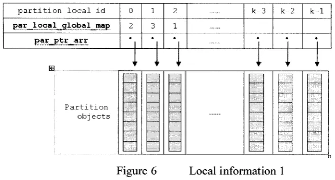
• The local information for partitions in a mesh is illustrated by Figure 6. The
par_local_global_map is actually an array which contains all local partitions’
global id. The indexes of the array stand for local ids of partitions. This means
that we can get each partition’s global id as long as we know a partition’s local id.
p a r t i t i o n l o c a l i d 0 1 2 k - 3 k - 2 k - 1
par_loca l__g 1 ob a l_map 2 3 1
par_ptr arr • • •
’r ' < ir < ’ '' 'r
H
P a r t i t i o n o b j e c t s
Figure 6 Local information 1
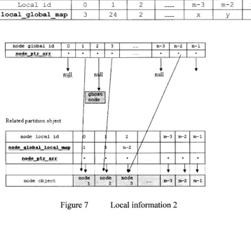
• Local information for nodes in a mesh is illustrated by Figure 7. The data member
local global map is an array which contains the global id of each local node. The
Local id 0 1 2 m-3 m-2 m-1
l o c a l g l o b a l m a p 3 24 2 X y z
node global id n-3 n-2 n-1
arr
null n i 11 null
R e la te d p a rtitio n o bject
node local id m-3 m - 2 m-1
node global local man
WVyAViWM\n-V-/.VVVVvV\ii*.\'1VAVV'//4i*/'/'A-\*v n-2
node »d£ node n o d e o b j e c t
Figure 7 Local information 2
5.3.2 Partition Structure
Partition is the basic load balancing unit in over-partitioning algorithm, which
stands for a sub-graph of the local mesh and the local mesh is a sub-graph of the whole
data graph.
Partitions track all information about nodes which belong to it, see Figure 7. The
array node_global_id_arr records all lo ca l n o d e s ’ glob a l id. M ean w h ile the pointer array
node_ptr_arr contains all pointers that point to all the nodes of the partition. The array is
used during the computation stage when we need traverse nodes one by one for each
5.3.3 Node Structure
Node data structure stands for a particle in a particle system or a vertex in a data
graph. An internal node data structure includes basic information about itself: global id,
local id, neighbor node information and edge-weight information. All of these are
necessary for Zoltan to manage partitioning and migration. Considering migration cost
and system scalability, the node structure should be kept as small as possible.
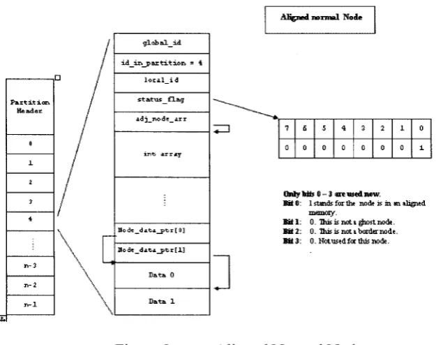
The node structure includes two parts: the first is the general information for
partition and migration; the second part is the node data for the computation. A node may
be a normal node, border node, or ghost node. A normal node is illustrated in Figure 8.
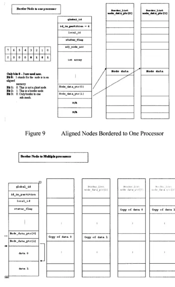
Border nodes and ghost nodes need more effort in handling because borders and ghosts
need to exchange information among processors. In order to avoid unnecessary data
copies for the communication phase, border nodes’ data is stored directly in the border
list (see Figure 9), except borders which are adjacent to more than one remote processor
(see Figure 10). Data member status _Jlag is used to track the type of current node:
1. status J la g data member of a node is of char type with a byte long, which is used to
record a node’s status. Now only bit 0 to 3 are used:
• Bit 0, stands for if the node is aligned. If this bit is set to 1, it means that current
node is in a continuous memory block.
• Bit 1, stands for if the node is a ghost node. If the bit is set to 1, it means the
• Bit 2, stands for if the node is a border node. If the bit is set to 1, it means the
current node is a border node.
• Bit 3, used by border nodes. If both this bit and bit 2 are set to 1, it means that
current node is bordered to multiple processors.
A lig n ed n o r m a l N ode
B o r d e r N ode to o n e p ro c e s s o r
7 6 S 4 3 2 1 0
0 0 0 0 0 1 0 1
Only bits 0 - 3 are used now.
B it 0 : 1 stands for the node is in an aligned
memory.
B it 1: 0. This is not a ghost node.
B it 2 : 1. This is a border node.
B i t3: 0 . O nlybordertoone sub-mesh.
Figure 9 Aligned Nodes Bordered to One Processor
id_in_part.itd.on = 4
status_flag
a d j _ n o d e _ a r r
N o d e_ d sta _ p t-r (0 ] N o d e _ d a ta _ p tr 113
n o d e _ d a f c a j r t r [0 ]
Node data Node data
B o rd e r N ode to M u lfy le pro cesso rs
I*
g l o b a l _ ± d x d _ x n _ p a x t x t x o n
s t a t u s _ f l a g
Mode_dita_ptr[ 0]
Mo de _ d a t i _ p t - r [ 1]
C opy o f d a t a 0 C opy o f d a t a 1
C opy o f d a t a 0 Copy o f d a t a 1
5.3.4 Borders and Ghosts
Border and Ghost cell management are very important to reduce network latency
during computation process. Borders are those nodes which have neighbor nodes located
on remote processors, and ghosts are copies o f border nodes on other processors. In other
words, they are simply images of border nodes on other processors. Border and ghost cell
management is used for communication because after each computation round, we need
to update values of ghost cells for the next computation round. Updated values of border
cell will be sent to corresponding remote processors to update those ghost cells. Borders
and ghost cells need to be rebuilt after each mesh adaptation.
Border and ghost cell management includes two stages: build/rebuild stage and
update stage. After each mesh adaptation, global location of some nodes will be changed,
some border nodes will no longer be border nodes as they do not have any neighbors on
remote processors; some local nodes become new border nodes because their neighbor
nodes have been migrated to other processors. So a rebuild needs to be done before
starting the next round of simulation computation. During simulation, after each round of
computation, the data values for each node are changed but these changes only take place
for local nodes. Since border nodes change too, their images in ghost cells need to be
P r o c e s s o r id 0 1 2 3 13 14 15
border list ptr arr
Vv\W^vVW'W,Yrt'A'¥attW"V«ttvWV'.'V ■ ■ ■ ■ ■ ■ ■
ni
border list object
VA\M*W/<WVM J
i l l
'
null null pull
Border list objects
Figure 11 Border List Structure
To maximize performance of our system each local mesh keeps a border table, see
Figure 11, which is a number of arrays with each array standing for border information to
a specific remote processor. On the other hand, each local mesh has only one array of
ghost nodes. Technically the array of ghost nodes has the same structure as other normal
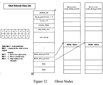
partitions except ghost nodes inside the partition need special treatment for their data, see
G host N ode an d G host List
O nly Infe 0 - 3 a re u s e d now. RttO : 1 stands fa r the node is in m dinned
m an o iy .
B it 1 B it 2 B it 3
1. This is n o t a. ^aost node. 0. H u sis a.border node. 0. Only'border to one
sub-mesh.
g lo b a l _ i d i d ir> p ax t i t i o n = 4
s t a t ms _ f l a g ad j _ n o d e _ a r r
Ho d e _ d a t a _ p t r [ 0] Wo d « e _ d a t a _ p t r [ l]
Ghos t_L is t node data_ptr[0]
Node data
..
GKos t_L is t
o d e _ d a ta _ p t x [1 3
Node data
Figure 12 Ghost Nodes
5.4
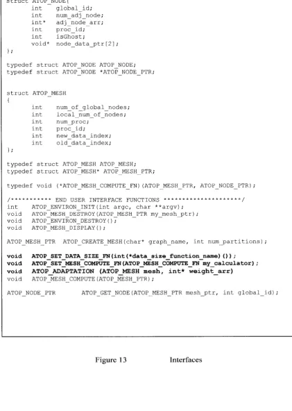
Interfaces
To separate general user-level application data structures from our internal data
structures, we design and implement a set of simplified interfaces, seeing Figure 13. By
hiding all the complicated details like environment initialization, data migration and load
balancing, simplified interfaces are provided. This approach can also make the runtime
system more extendable and maintainable.
These interfaces have been loosely tied to users’ development style. Users can
have their own node data structures without worrying about how the system handles them.
For example, particle node data can be as simple as just an integer or a user-defined
relation to other nodes. The requirement from the system is that the user has to bind the
user-defined information to the system by calling a couple of call-back functions. One
advantage of our interfaces is that users do not need deal with communication manually.
All communication among processors are handled automatically by the library.
Applying the interfaces to real simulations is simple. A programming example of
particle simulation is shown in Appendix 3, which is also the basic application used for
our experiments in Chapter 6. Using the library generally includes the following steps:
1) First, a user defines his or her node data structure and ties it to the system by
using the callback function A T O P _ S e t _ D a t a _ S i z e _ F n ( & n o d e _ d a t a _ s i z e ) ;
2) Second, the user defines his or her computation function and ties it to the system
by using callback function
A T O P _ S E T _ M E S H _ C O M P U T E _ F N ( A T O P _ M E S H _ C O M P U T E _ F N m y _ c a l c u l a t o r ) ;
3) Then the mesh, and computation environment is initialized;
4) An adaptation can be performed by calling a t o p_ a d a p t a t i o n ( M e s h _ P t r m e s h ,
I n t * c o m p u t _ w e i g h t _ a r r ) ;
5) Repeatedly a t o p_m e s h_c o m p u t e (a t o p_m e s h_p t r) is called to do mesh computation;
or the user goes back to step 4) to make another adaptation if it is necessary; or
goes to step 6) if the simulation is finished;
struct ATOP NODE { int global id; int num adj node ; int* adj node arr; int proc id; int isGhost;
void* node data ptr[2
} ;
typedef struct ATOP_NODE ATOP_NODE; typedef struct ATOP_NODE *ATOP_NODE_PTR;
struct ATOPJMESH
{
int num of global nodes int local num of nodes; int num proc;
int proc id;
int new data index; int old data index; } ;
typedef struct ATOP_MESH ATOP_MESH; typedef struct ATOP_MESH* ATOP_MESH_PTR;
typedef void (*ATOP_MESH_COMPUTE_FN)(ATOP_MESH_PTR, ATOP_NODE_PTR);
/*********** END USER INTERFACE FUNCTIONS *********************/ int ATOP_ENVIRON_INIT(int argc, char **argv);
void ATOP_MESH_DESTROY(ATOP_MESH_PTR my_mesh_ptr); void ATOP_ENVIRON_DESTROY();
void ATOP_MESH__DISPLAY () ;
ATOP MESH_PTR ATOP_CREATE_MESH(char* graph_name, int num__partitions);
v o i d A T O P _ S E T _ D A T A _ S I Z E _ F N ( i n t ( * d a t a _ s i z e _ f u n c t i o n _ n a m e ) ( ) ) ;
v o i d A T O P _ S E T _ M E S H _ C O M P U T E _ F N ( A T O P _ M E S H _ C O M P U T E _ F N m y _ c a l c u l a t o r ) ;
v o i d A T O P _ A D A P T A T I O N ( A T O P _ M E S H m e s h , i n t * w e i g h t _ a r r )
void ATOP_MESH__COMPUTE(ATOP_MESH_PTR);
ATOP_NODE_PTR ATOP_GET_NODE(ATOP_MESH_PTR mesh_ptr, int global_id);
5.5
Memory Alignment
Memory alignment is the core of the data locality management. For a mesh or a
graph, the nodes usually are generated dynamically, which means those nodes are always
spread in memory, see Figure 14. But after finishing memory alignment, all nodes for a
partition are located in one memory block and can be accessed sequentially. During the
partitioning stage, the number of partitions for the whole global mesh can be chosen, and
the memory size of a partition can be adjusted. The appropriate size for the partition
located in a continuous memory block can take advantage of the cache performance and
finally enhance throughput of the whole application.
m-3 m-2 m-1
n o d e l o c a l i d
n - 2
n o d e n o d e
m -1 rrt-2
Figure 14 Un-aligned Partitions
When aligning memory for a partition, the memory management module will only
put the partition header information and all corresponding nodes in one continuous
memory block. A good reason for this structure is future extension. Right now Zoltan can
o n ly m igrate n o d e s but can not m igrate partitions directly. H o w ev er, k eep in g all partition
information together provides an opportunity to migrate partitions individually in the
la
n o d e l o c a l i d 0 1 2 m-3 m- 2 m -1
n o d e _ g 1o b a l _ i d _ a r r 1 3 n - 2
n o d e _ j s t r _ a r r • • • • •
r *' : i ' ' ’
i.: r lp d « ! :: irlnoditlii a i & a s i : : ;
i r u : . ,r2 ' : : ’ I m- 3 m-2 m-1
□
6
Experimental Results
6.1
Experimental Environment
We perform all our experiments on an IBM cluster, which includes 16 nodes, and
each node contains dual Intel Xeon processors with 512 Mbytes of RAM. All nodes have
2.2 GHz CPU except the two nodes which have 2.4 GHz CPUs. Nodes are connected by
Myrinet high-speed interconnect. The operating system is Debian Linux with 2.6 Kernel
on each node, the MPI package we used is MPICH 1.27, the Zoltan version is 2.1 and the
ParMETIS is version 3.1, and K-way partition algorithm is used.
Graphs |V| |E| Description
3elt 4720 13722 2D finite element mesh
4elt 15606 45878 2D finite element mesh
wing 62032 121544 3 finite element mesh
brack2 62631 366559 3 finite element mesh
fman512 74752 261120 N/A
wave 156317 1059331 N/A
Table 1 Benchmark Graphs
W e c h o se the benchm ark graphs from U n iv ersity o f G reen w ich Graph Partition
Archive [26], all with Chaco graph file format. This graph archive contains various types
of graphs which fit our test plan. For better comparison we choose those test graphs
as graph finan512 and three times as many edges as graph brack2, was chosen to test the
scalability of our runtime system.
6.2
Adaptation Performance
As we mentioned, ATOP is used in our system to manage partitioning and load
balancing, however, new data structures were designed to achieve higher performance
and avoid un-necessary search for nodes which existed in the original ATOP
implementation. So we use the same set of graphs used in [20] to do our experiments in a
space-shared environment and a time-shared environment to get comparable
experimental results.
6.2.1 Adaptation Experiments in a Space-shared Environment
Both Table 2 and Table 3 show experiments in a space-shared environment.
When using ATOP over-partitioning algorithm, graphs were partitioned into 8 partitions
initially and number of processors changed in an order 4 - 8 - 4 - 2. Shaded rows are
data from [20], and all data is in seconds. The init time includes time for creating graphs
by reading graph files from hard drives and time for initially partitioning and migration to
4 processors. The adaptation time is the total adaptation time for the three adaptations (4-
>8, 8->4 and 4->2).
The data shows big jumps in performance. Table 2 shows that the init time for
over-partitioning can be shortened by 93% to 98.7% from these graphs, and adaptation
illustrates that init time for partitioning from scratch can speed up by 94% to 99%. For
over-partitioning, the adaptation time for partitioning from scratch can be improved by
63% to 75%. The difference of edge cuts is because we used a new version of Zoltan.
Graphs
Overall Edge Cuts
Init Time Adaptation Time
4 8 4 2
wing
2390 3261 2390 1858 202.3 25.8
2428 3287 2428 1858 12.1 2.3
38 26 38 0 -189.9 -23.5
Speedup 94% 91.1%
brack2
5047 8528 4069 204.1 26
3893 8197 3893 2907 12.7 2.4
-1154 -331 -1154 -1162 -191.4 -23.6
Speedup 93% 90.7%
flnan512
405 648 405 ; 296.0 49
405 648 405 324 3.9 2.0
0 0 0 0 -292.1 -47
Speedup 98.7% 95.9%
Table 2 Adaptation by over partitioning in space-shared environment with 8 partitions
Table 4 and Table 5 illustrate init time and adaptation time comparison for 16
partitions and experiments executed on 16 processors. More graphs are tested and the
adaptations follow 8 - 1 6 - 4 - 2 processor sequence. Init time includes initial mesh
Similarly the shaded data come from [20] and all the rest is from current experiments.
The results show that, for small sized graphs like 3elt and 4elt, our approach does not
gain any advantage. But if the size of the graphs becomes bigger, the optimized data
structures contribute greatly to the whole init and adaptation performance. Figure 16 and
Figure 17 illustrate our performance enhancement in graphic form, where OP stands for
current results.
Graphs
Overall Edge Cuts
Init Time Adaptation Time
4 8 4 2
2129 3081 2036 947 f 215.3 ; 102.7
wing
2325 3087 2186 999 11.8 32.3
196 6 150 52 -203.5 -70.4
Speedup 94.5% 67.5%
3163 8221 223.0 88.8
brack2
3159 8222 2972 754 12.7 33.0
-4 1 -141 7 -210.3 -55.8
Speedup 94.3% 62.8%
324 648 162 328.7 199.8
finan512
324 648 324 162 3.9 50.8
0 0 0 0 -324.8 -149
Speedup 98.8% 74.5%
Table 3 Adaptation by partitioning from scratch in space-shared environment with
Table 6 and Figure 18 show init time and adaptation time comparison with 128
partitions by using over-partitioning. Initially the experiments were running on 8
processors, and then adapted to 16, 4 and 2 processors respectively. The results show our
optimized implementation has speedup up to 99% for init time and speedup up to 96%
for adaptation time. This proves that our implementation can also achieve better
performance for large number of nodes. Larger number of partitions does not affect our
system’s performance.
3elt 4elt wing brack2 finan512
INIT TIME 0.2 0.5 3.3 1.2 210 12.1 ;ii222 12.7 312 3.9
AP TIME 0.1 0.2 0.5 0.4 20.3 2.0 22.6 2.1 38.0 2.1
Table 4 Init time and adaptation time by over-partitioning for 16 partitions
3elt 4elt wing brack2 finan512
INIT TIME 0.3 0.3 3.6 1.2 234 11.8 245 12.7 354 3.9
AP TIME 0.2 0.4 2.2 ; 2.2 61.5 34.2 56.5 31.1 113 50.5
Table 5 Init time and adaptation time by partitioning from scratch for 16 partitions
3elt 4elt wing brack2 finan512
INIT TIME 0.4 0.4 4.1 1.0 215 10.5 224 11.5 326 2.8
AP TIME 0.2 0.4 0.4 17.5 1.2 18.1 1.2 30 1.0
16 partitions with ATOP
350
300 4-
250
2 00 4-
150
T
100
50
j-o
i-3elt 4elt wing brack2 finan512
init time
h»— init time(OP) adapt time
-x— adapt time(OP)
Figure 16 Comparison for 16 partitions by ATOP
16 Partitions with Partitioning from Scratch
40 0 r
350
300
250
200
150 |
100
j-5 0 ■
0 r
3elt wing brack2 finan512
init time
Hu— init time(OP)
adapt time
adapt time(OP)
128 Partitions with ATOP
350
300
---25 0
j--200 —
-150
j--1 0 0
---50
j
-0 - — T
init time
init time(OP)
adapt time
x, adapt time(OP)
3elt 4elt vwng brack2 finan512
Figure 18 Comparison for 128 partitions by ATOP
6.2.2 Adaptation Experiments in a Time-shared Environment
In order to test our system in a time-shared environment, we assign each
processor with different computation weight to simulate changed time shares. Initially
we set up 8 processors with relative computation weights 2:2:2:2:1:1:1:1, then the
weights changed to 1:1:1:1:1:1:1:1 -> 1:1:1:1:2:2:2:2 -> 1:1:1:1:2:2:3:3 respectively.
Table 7 and Table 8 show the experiment results for using ATOP over-partitioning
algorithm and using partitioning from scratch by using K-way partitioning respectively.
Table 7 and Table 8 show that our optimized implementation also provides
improvement in a time shared environment. The bolded columns stand for the speedups.
Init time gains up to 99% speedup for both over-partitioning and partitioning from
Adaptation time by over-partitioning in our implementation can reach a speedup to 97%
and the adaptation time by using K-way partitioning from scratch can get up to 72%
improvement.
Init 1:1:1:1:1:1:1:1 1:1:1:1:2:2:3:3
wing 221.9 10.7 95% 3.92 0.26 93% 458 0.24 95% 0.91 0.13 85%
brack2 12.3 94% 3.72 0.38 90% 4.48 0.72 84% 0.93 0.42 55%
finan512 2.94 99% 4.33 0.19 95%
M lE
0.21 97% 0.10 0.10 0Table 7 Init time and adaptation time by ATOP environment with 128 partitions
Init 1:1:1:1:1:1:1:1 1:1:1:1:2:2:2:2 1:1:1:1:2:2:3:3
wing 226.93 10.63 95% 22.05 6.87 67% 29.49 8.22 72% 1.87 9.05 -384%
brack2 229.98 11.58 95% 25.80 7.02 73% 24.56 8.41 66% 2.10 10.40 -395%
finan512 354.52 2.83 99% 23.18 8.66 63% :::24f4'" 10.5 57% 3.2 12.36 -286%
Table 8 Init time and adaptation time by K-way Partitioning from scratc
partitions
6.3
Data Locality Management Module Performance Experiments
The locality management module plays the most important role in our system and
deserves separate experiments to test it. Currently this module is implemented by using
memory alignment. In order to test performance of this memory alignment, we need a test
scenario which includes typical particle simulation data structures and a particle
computation function.
As we discussed in Section 5.4, our implementation allows users to define their
own node data structure and solver computation functions. Then they can use call-back
functions to tie their own functions with our runtime system. For this experiment, we use
a very simplified node data structure and computation functions like below:
double node_data[2];
node_data [x] = (^neighbor_node [x]) /number_of_neighbors (5)
node_data [y] = (^neighbor node [y]) /number_of_neighbors (6)
Each node has two dimensional floating-point data and the computation functions
are calculating the average values of all the neighbor nodes’ data in two coordinate values
respectively. Then the newly calculated data will be used for the next computation round.
Each node needs access to its neighbor nodes’ data to finish computing its position for
the next step. After computation, the local processor will communicate with other
The locality management module experiment is done in two steps: First we test
the performance of memory alignment in a static environment without any adaptation.
Then we conduct our experiments in a dynamic environment where the system induces
dynamical resource changes to simulate a real space-shared and time-shared runtime
environment.
6.3.1 Computation Time in Static Environment
First we test the performance enhancement from memory alignment in a static
environment, in which we use eight processors, 128 partitions and with processor relative
weights {1,1,1,1,1,1,1,1}, which means we run the experiments on 8 processors and each
processor provides the same time share for the experiments. In other words, the weight
stands for computation time. For each experiment the number of iterations will be 1000,
5000, and 10000 respectively. All data is in seconds.
Graphs/ Iterations 1000 5000 10000
Name i n iei Time speedup Time speedup Time speedup
wing
|V| =62032
|E| = 121544
26.95 29.3% 125.6 22.7% 257.0 29.7%
19.04 97.04 180.60
brack2
|V| =62631
|E| = 366559
24.35 13.2% 121.58 11.7% 245.12 12.2%
21.13 107.41 215.30
wave
|V| -156317
|E| = 1059331
62.84 14.3% 319.52 15.9% 653.89 16.4%
53.87 268.80 546.60
Table 9 illustrates the test result, where the shaded cells contain normal
computation time without memory alignment, and the non-shaded cells are computation
time with memory alignment. All numbers are in seconds. In this table we can see that
our memory management successfully shortens computation time by 11.7% to 29.7%.
Different iteration time also shows that the enhancement is steady and the module has no
slow-down when the graph’s size becomes larger. Figure 19 also shows these
improvements in separate charts.
norma
Haigrned
10000
B norm al ■ a lig im e d
10000