ABSTRACT
ELLIOTT, CHRISTOPHER MARK. Methods for Streamlined Firefly Optimization and Interpretation: Applications to Electromechanical Systems Design (Under the Direction of Gregory D. Buckner).
This dissertation introduces methods for optimal engineering design and for exploration of the design space. The applications explored involve the design of electromechanical devices, in addition to benchmark problems. Two methods are introduced: a computationally efficient variation of firefly algorithm (FA), tuned to find multimodal objective function minima; and a new method for programmatically and visually identifying locally optimal solutions. The visualization method, a plot of distances between cost-sorted designs (the cost-sorted distance
Methods for Streamlined Firefly Optimization and Interpretation: Applications to Electromechanical Systems Design
by
Christopher Mark Elliott
A dissertation submitted to the Graduate Faculty of North Carolina State University
in partial fulfillment of the requirements for the degree of
Doctor of Philosophy
Mechanical Engineering
Raleigh, North Carolina 2017
APPROVED BY:
________________________________ ________________________________
Dr. Gregory D. Buckner Committee Chair
Dr. Larry M. Silverberg
________________________________ ________________________________
DEDICATION
BIOGRAPHY
ACKNOWLEDGMENTS
TABLE OF CONTENTS
LIST OF TABLES ... VIII
LIST OF FIGURES ... IX
LIST OF ALGORITHMS ... XIII
CHAPTER 1 INTRODUCTION... 1
1.1 Background and Motivation 1.2 Research Objectives ... 4
1.3 Organization ... 5
CHAPTER 2 METHODS FOR STREAMLINED FIREFLY OPTIMIZATION AND INTERPRETATION: APPLICATION TO ENGINEERING DESIGN ... 6
2.1 Introduction 2.2 Methods... 10
2.2.1 Firefly Algorithm Implementation 2.2.2 The Cost-Sorted Distance Method ... 14
2.2.3 Identifying CSD Cluster Champions ... 16
2.2.4 Configurable Benchmark Function... 18
2.2.5 FA Parameter Tuning ... 21
Benchmark Optimization: 1D, 2D, 3D, and 4D ... 26
2.3 Example: Electromechanical Design Optimization ... 33
2.3.1 Active Magnetic Bearing and Controller 2.3.2 FA Optimization of AMB+PID Design Parameters ... 36
2.4 Discussion/Conclusions ... 39
3.1 Introduction
3.2 Methods for Quantifying Robustness ... 44
3.2.1 A Deterministic Approach 3.2.2 Monte Carlo Approach ... 47
3.2.3 Probability of Dominance ... 49
3.2.4 Correlation Between Robustness Measures and the Fireflies Clustered ... 51
3.3 Results ... 54
3.4 Discussion/Conclusions ... 59
CHAPTER 4 DESIGN OPTIMIZATION: ELASTOMERIC BAFFLE MRFD ... 60
4.1 Introduction 4.2 Methods... 66
4.2.1 Magnetic Circuit Model ... 68
4.2.2 Electrical Circuit Model ... 71
4.2.3 Mechanical System Properties ... 72
4.2.4 Material Properties ... 73
4.2.5 Design Optimization ... 75
4.2.6 FEA Validation ... 81
4.2.7 Prototype Development ... 82
4.2.8 Experimental Validation ... 84
4.3 Results ... 85
4.4 Discussion/Conclusions ... 95
CHAPTER 5 CONCLUSIONS ... 97
5.1 Future Research Opportunities ... 98
REFERENCES ... 99
APPENDICES ... 107
APPENDIX A: ACTIVE MAGNETIC BEARING MODEL ... 108
APPENDIX C: EXPERIMENTS TO MEASURE B VS H ... 116
APPENDIX D: MRFD PERFORMANCE EXPERIMENTS ... 118
LIST OF TABLES
Table 2.1 The 10 lowest cost results from a full-factorial FA parameter search. ... 26
Table 2.2 Summary of 1D-4D benchmark optimization results. Optimization was completed for 1000 each of 1D, 2D, 3D, and 4D randomized benchmark problems. ... 32
Table 2.3 FA optimization champions and associated of the engineering design example. ... 37
Table 3.1 Robustness measures, (3.7) minima ... 51
Table 3.2 linear correlation measures for vs ... 56
Table 3.3 linear correlation measures for PFF vx. PoD. ... 59
Table 4.1 Parameters of (4.2), corresponding to Figure 4.8.b. ... 70
Table 4.2 Optimization variables are a partially modified version of the design parameters with the addition of magnetic flux density ... 76
Table 4.3 FEMM settings for solving the magnetic field problem using FEA ... 82
Table 4.4 The optimization variables, their units, firefly lower and upper limits, and optimal results after conjugate gradient optimization for each of the cluster champions of Figure 4.18. ... 90
Table 4.5 Important results for the designs of Figure 4.19. ... 91
Table 4.6 Predicted | | for the optimal design. ... 93
Table A.1 Parameters of (4.2), corresponding to Figure 4.8.a. ... 114
LIST OF FIGURES
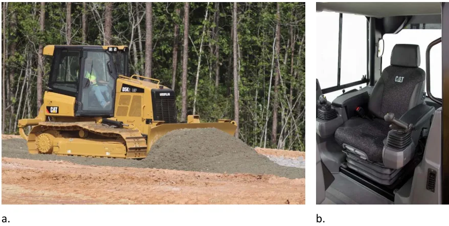
Figure 1.1 a. A drive-by-wire construction machine. b. The operator station with adjustable,
seat-mounted, electronic joysticks. Images courtesy of Caterpillar. ... 2
Figure 2.1 Equation (2.4) for five different values of α. ... 13
Figure 2.2 Histograms indicating distributions for the output of (2.4) ... 14
Figure 2.3 a. A typical 2D cost function contour plot with fireflies (white data points) in their final migration positions – fireflies have clustered near three local minima; b. CSD plot ... 15
Figure 2.4 CSD plot views ... 17
Figure 2.5 Examples of a. 1D, b. 2D, and c. 3D cost functions from (2.5) with randomly generated parameters. ... 20
Figure 2.6 Averages and standard deviations from 25 batches of cost_x as functions of the number of optimizations in each batch for fixed FA tuning parameters ... 25
Figure 2.7 1D cost function (2.5) with initial and final firefly positions and corresponding CSD plots. .... 27
Figure 2.8 2D cost function (2.5) with initial and final firefly positions and corresponding CSD plots. .... 29
Figure 2.9 3D cost function (2.5) with initial and final migration firefly positions and corresponding CSD plots. ... 30
Figure 2.10 4D cost function (2.5) with initial and final firefly positions and corresponding CSD plots. .. 31
Figure 2.11 Schematic of a longitudinal AMB, where the separation between stator and mover is maintained by a PID controlled coil voltage. ... 34
Figure 2.12 AMB design example with initial and final CSD plots and designs resulting from firefly optimization. Table 2.3 provides detail regarding the champions and related performance measures. ... 36
Figure 2.13 Transient simulation results ... 38
Figure 3.1 An example of the simplest possible multimodal objective function. ... 47
Figure 3.2 Uncertainty propagation for each of two minima of a typical 1D benchmark function. ... 49
Figure 3.4 Typical 2D optimization results. In each plot, champions are labeled 1 through 4 from lowest
to highest objective function value. ... 53
Figure 3.5 PFF vs. PR: histograms of slopes from least-square-error line fits. Estimated probability density and cumulative probability distributions are also shown. ... 55
Figure 3.6 PFF vs. PR: all data points from 1000 firefly optimizations of randomized benchmark functions. ... 56
Figure 3.7 PFF vs. PoD: histograms of slopes from least-square-error line fits. ... 57
Figure 3.8 PFF vs. PoD: all data points from 1000 firefly optimizations of randomized benchmark functions. ... 58
Figure 4.1 Examples of pressure-driven and direct shear modes for MRFDs. ... 61
Figure 4.2 Three examples of MRFD types: ... 62
Figure 4.3 An absorbent matrix MRFD. ... 65
Figure 4.4 The elastomeric baffle MRFD design. ... 66
Figure 4.5 Some practical details of the elastomeric baffle MRFD design ... 67
Figure 4.6 Parameterized spool and housing geometry used for design optimization... 67
Figure 4.7 Lumped parameter magnetic circuit model. Magneto motive force drives magnetic flux through a series of n reluctances. ... 68
Figure 4.8 Detailed parametric geometry for a magnetic circuit model corresponding to Figure 4.6. Evaluation of one-quarter of the cross-section is sufficient due to symmetry of the design. ... 69
Figure 4.9 Lumped parameter electric circuit model. Voltage source drives current through a series of resistance and inductance. ... 71
Figure 4.10 Shear parametric dependencies of MRF ... 74
Figure 4.11 Magnetic parametric dependencies of MRF and low-carbon steel ... 75
Figure 4.12 The magnetic circuit model results in a transcendental set of equations. ... 77
Figure 4.13 A benchmark 2D cost function and the corresponding CSD plot. ... 81
Figure 4.14 Solid model images of the prototype MRF damper. ... 83
Figure 4.15 A photograph of the prototype MRFD. ... 84
Figure 4.17 Results summary for the modified firefly portion of Algorithm 2.1. ... 86
Figure 4.18 Distances (Euclidean norms) of fireflies from the lowest cost result, for the last migration. .. 87
Figure 4.19 Cost and geometry of the five cluster champions from Figure 4.18 (blue) and their conjugate
gradient optimal counterparts (red). ... 89
Figure 4.20 FEA result for the best design from Table 4.5 showing |B| contour lines in the ferromagnetic
spool and housing. ... 92
Figure 4.21 a. Cross-section of the spool and housing showing locations sampled for FEA results in Table
4.6. b. FEA predicted |B| in the MRF, between piston and cylinder. ... 93
Figure 4.22 Cyclic joystick motion with current commands from 0 to 0.5 A in 10 steps: a. force vs. time
and b. force vs. displacement. ... 94
Figure A. 1 Electromechanical energy conversion is modeled with a lossless magnetic field coupling
electrical and mechanical subsystems. ... 108
Figure A. 2 Magnetic field energy is assumed a function of states and . ... 110
Figure A. 3 Lumped parameter electric circuit model. ... 111
Figure A. 4 A research assistant records data to characterize B vs. H for a ferrous material. ... 116
Figure A. 5 Schematic for measurement of sample B-H curve. ... 116
Figure A. 6 Material sample dimensions (mm). ... 117
Figure A. 7 A research assistant actuates the MRFD to measure device performance. ... 118
Figure A. 8 Six seconds of typical MRFD force and displacement data. ... 119
Figure A. 9 Assembled MRFD parts. ... 120
Figure A. 10 The ferrous cylinder built to the optimal geometry specified in Table 4.4. ... 121
Figure A. 11 The optimal ferrous spool with geometry specified in Table 4.4. ... 122
Figure A. 12 Two of these aluminum shafts are used to suspend the spool ... 123
Figure A. 13 These non-ferrous caps are attached to either end of the ferrous housing ... 124
Figure A. 14 A spacer for the rolling elastomeric baffle. ... 125
Figure A. 15 A “swabable” check valve used for injecting/removing MRF by syringe. ... 126
Figure A. 16 Stainless steel adapter compatible with the check valve shown in Figure A. 15. ... 126
Figure A. 17 This spherical bearing secured the MRFD to the base block as shown in Figure A. 9. ... 127
Figure A. 18 A force sensor was threaded between a rod end and the shaft shown in Figure A. 12. ... 128
LIST OF ALGORITHMS
Procedure 2.1 Tuning FA parameters for a broad class of optimization problems. ... 22
Algorithm 2.1 Enhanced FA pseudo code. ... 11
Algorithm 2.2 Random additional motion applied to fireflies in step 5.2.2 of Algorithm 2.1. ... 12
Algorithm 2.3 The histogram approach used in step 5.4.1 of Algorithm 2.1 to identify cluster champions.
... 18
Algorithm 2.4 A function for quantifying the extent to which a set of design vectors have converged near
the seeds of the function . ... 23
Algorithm 4.1 Optimization pseudo code. ... 79
Chapter 1
Introduction
1.1
Background and Motivation
a. b.
Figure 1.1 a. A drive-by-wire construction machine. b. The operator station with adjustable,
seat-mounted, electronic joysticks. Images courtesy of Caterpillar.
Caterpillar’s small track-type tractor (shown in Figure 1.1) became fully drive-by-wire in the early 2000s. However, digital drive-by-wire (or fly-by-wire) control was originally developed for aerospace applications in the 1950s-1970s. The first piloted system demanding fully fly-by-wire control (as opposed to mechanical operator control, tele-operator control, or completely automatic computer control, which were all used in the same timeframe) was NASA’s lunar module, built in the 1960s. The vehicle was designed to be piloted by a computer guidance system, but with the ability for the human pilot to intervene (incidentally, this feature was crucial to the success of the Apollo moon landings – even preventing an aborted mission on the first lunar landing [1]). The lander provided electronic, rather than mechanical, operator override. NASA proceeded in the 1970s to develop fully fly-by-wire aircraft control [1] and many such aircraft systems have since been developed.
aircraft, flown in 1958. Due to the extreme performance demanded of this airplane, computer augmented yaw control was necessary to provide stable operation. The pilot interface was at first made without an attempt to emulate traditional mechanically controlled flight systems. However, to gain pilot acceptance, it later had to be modified with springs to emulate the feel of cable control [1]. A similar experience was had for NASA’s fully fly-by-wire system, as documented by Tomayko, “This system had no feedback to the pilot, so a set of springs, bobweights, etc., was arranged to give artificial “feel” similar to that in a cable-only control system… In the early days of fly-by-wire, engineers thought that such an artificial feel system would be unnecessary, probably reasoning that the electronic feedback would be sufficient for control.” [1].
Iteration of this sort is to be expected with the transition from mechanical to electronic control interfaces. Haptic feedback is inherent in many mechanical interfaces, so designers updating to digital control may be unaware of it, fail to fully appreciate the role it serves, or may even view it as a problem to be solved (for example, if force feedback causes operator fatigue). With drive-by-wire digital control, haptic feedback must be intentionally created by the system designer and it is likely to be lacking if the designer has not explicitly considered it.
Another problem encountered by NASA in development of fly-by-wire is unwanted feedback. Biodynamic feedthrough or operator induced oscillation (OIO) [2] is machine vibration where the operator unwillingly participates in unstable closed-loop command feedback. This happens when the machine accelerates the operator in a mode and at a frequency that he or she cannot avoid passing motion through the input device. It is a common nuisance for many machines, but can have devastating consequences in aircraft control where sustained or escalating oscillation and can lead to loss of control. OIO may be mitigated by reducing the efficiency of the feedback path e.g. by better isolating the operator from the machine or the machine control from the operator. This remains an active research topic (e.g. [3], [4], [5]).
develop advanced design optimization methods that can be applied to an electronically controllable magnetorheological fluid device (MRFD) suitable for these purposes.
Designing electromechanical devices and other similarly complex engineering systems can be challenging. Methods for predicting a design’s performance are often either computationally prohibitive or overly simplistic; and predicting a given design’s performance is usually a small part of the challenge. The designer must solve the inverse of this problem, which is to select the design that gives the best performance possible. This requires a method for predicting any
feasible design’s performance (usually a parameterized, many-degree-of-freedom model), and a way of intelligently choosing from the, perhaps infinite, design set. Furthermore, the meaning of “best performance possible” may not be straightforward. Real world designs are almost always the result of compromises between multiple conflicting performance measures. The goal of this dissertation is to develop and demonstrate an optimal design tool set to address these challenges.
1.2
Research Objectives
The overall goal of this research is to develop and demonstrate methods for optimal engineering design, and ultimately to use these methods to design a novel MRFD. The specific objectives are to:
1. Develop a new firefly algorithm (FA) suitable for multimodal optimization. 2. Demonstrate the cost-sorted distance (CSD) method for design space exploration. 3. Tune the FA to reliably cluster “fireflies” at multiple objective function minima. 4. Demonstrate FA optimization and CSD visualization for benchmark problems and
electromechanical system design.
5. Examine the usefulness of FA and CSD for design under uncertainty.
1.3
Organization
Chapter 2 introduces novel methods for optimal engineering design. A state of the art FA that incorporates recommendations from recent literature with further improvements described here is developed. A complimentary technique, the CSD method, for visualization and clustering is also introduced and demonstrated.
In Chapter 3, the extent to which FA and CSD are useful for addressing uncertainty in the design process is investigated. Various robustness measures are described and the hypothesis that the percentage of fireflies per cluster correlates linearly with robustness of the associated designs is tested.
Chapter 2
Methods for Streamlined Firefly
Optimization and Interpretation:
Application to Engineering Design
2.1
Introduction
Numerical optimization is often the only practical means for solving nonlinear engineering design problems with multiple degrees of freedom and conflicting objectives. Although sophisticated optimization methods for such applications have been developed, it can be difficult for a designer to use them to explore the design space. This chapter describes a methodology that can be used to easily identify and assess multiple attractive designs for these problems.
Design optimization can be facilitated by development of a scalar objective function of the design variables , , . . , which quantifies design fitness. By convention, a design is optimal if it minimizes and satisfies inequality and equality constraints, and :
subject to:
0, ∈ 1, 2, … 0, ∈ 1, 2, …
(2.1)
where is a scalar weighting factor. The objective and constraint equations may be combined to form a penalty function:
0, 0, | | (2.2)
where and are penalty factors used for inequality and equality constraint violations, respectively, and is the equality constraint convergence tolerance. Minimizing (2.2) is thus equivalent to solving (2.1).
Solutions to (2.1) or (2.2) may be approximated using a variety of optimization methods; gradient-based and population-based methods are two types commonly used. Gradient approaches [6] (e.g. steepest descent, conjugate gradient, Newton-based methods) can be effective for smooth, differentiable functions, but the rate and stability of convergence may be inferior to other methods for the multimodal or discontinuous cost functions frequently associated with multi-degree-of-freedom design optimization. Population-based methods [7] such as genetic algorithms, particle swarm optimization, and other nature inspired algorithms take advantage of large and diverse populations of solutions to overcome these limitations. The firefly algorithm (FA), introduced by Yang [8] in 2009, is a population-based optimization method inspired by firefly behavior, where design vectors ( ’s, the fireflies) migrate toward better fit neighbors in the design space. FA can be tuned to favor local solutions, rather than more exhaustively seeking the global optimum, and thus can be used to identify promising design alternatives. The core concept of FA is that the cost function of a design vector can be represented as the light intensity of a firefly: a design vector with a more favorable cost function is represented by a firefly with a brighter light intensity (i.e. ). At each design iteration, fireflies with lower intensities migrate toward brighter neighbors. The distance traversed is exponentially dependent on their spatial separation:
1 (2.3)
number; 1; and generates a vector of randomly distributed numbers, enhancing design space exploration.
Yang [8] discussed FA parameter tuning, compared and contrasted it with particle swarm optimization (PSO) and genetic algorithms (GA), and used 10 benchmark problems to demonstrate that FA can be superior to these alternative methods. Yang showed that FA converged to the global minimum in 99% of his simulations, 11% more often than GA and 6% more often than PSO, while requiring only 19% of GA’s function evaluations and 40% of PSO’s.
Improved versions of FA have been applied to a wide array of problems in recent years. Of note, Lukasik and Zak [9] in 2009 incorporated random variation in proportion to firefly distance from search space boundaries, and Yang [10] in 2010 proposed generating randomized step sizes from the Lévy distribution [11] (based on an inverse power law), providing a more thorough search of the design space. These improvements are incorporated in the algorithm developed here. Fister, et al. [12] in 2013 surveyed 172 articles related to FA, and documented avenues for continued research and development. The authors summarized FA method contributions and classified them as classical, modified or hybrid types. They also documented and categorized FA application examples from literature. In conclusion, they highlighted the method’s simplicity, flexibility and versatility, but noted that ideal FA parameter tuning can itself be a difficult optimization problem; more studies are needed to improve parameter specification.
methods typically involve identifying a Pareto frontier [15] of non-dominated designs from a large population of results. The Pareto frontier is a useful programmatic and graphical analysis tool for problems where the designer needs to understand trade-offs between two or more competing cost functions, but while a potentially infinite set of optimal designs can be identified, little information may be gained regarding dominated minima. In cases where population-based methods are capable of grouping design vectors near attractive solutions, these groups may be identified using clustering methods [16], which are optimization algorithms themselves, but can be computationally prohibitive.
In recent literature, tools to assist the designer in interpreting optimization results and finding attractive alternate designs have begun to emerge. Mattson and Messac [17] proposed a methodology for identifying attractive designs from multi-objective optimization results and demonstrated interactive software for down-selecting from the design space. Stump, et al. [18] developed “visual steering commands that help decision makers form their preference while exploring the trade space (i.e., “shopping”) to focus in on regions/points of interest as their preference sharpens.” Daskilewicz and German [19] proposed a set of features of interactive decision-support tools to promote effective and practical engineering design, and implemented these in an open-source computer program designed to be part of a user-in-the-loop optimization process.
for visually identifying local minima is introduced: a plot of the distances between cost-sorted fireflies (the “cost-sorted distance” or CSD plot). The CSD plot is shown to reveal clusters near local minima, making the best design associated with each cluster (the local champion) readily apparent to the designer. A methodology for tuning FA parameters is shown to achieve clustering of results at the objective function minima. Finally, the tuned algorithm is demonstrated using benchmark problems and a “real world” electromechanical case study.
2.2
Methods
This section details the FA enhancements for imparting random firefly motion, the CSD plot and its programmatic implementation, the parametric benchmark function used to tune FA, and the tuning method.
2.2.1 Firefly Algorithm Implementation
Algorithm 2.1 Enhanced FA pseudo code. , ,and are the FA tuning parameters that may vary with migration. Improvements relative to the literature are highlighted in red.
Parameters , , , , and affect convergence to local minima of cost function . The number of cost function evaluations is proportional to the number of fireflies and number of migrations . Parameters , , and can be fixed (in which case they are scalars) or be specified functions of the migrations (e.g. can be linearly interpolated between on the first migration and on the last migration, in which case they are vectors). The probability of significant random motion is determined by ; if it is large (e.g. 20) the probability is small
, , , , , , , ):
1. Given , a function of design vector , design vector limits and , the number of fireflies ,
the number of migrations , and firefly tuning parameters, , , ,
2. Initialize random fireflies , each within limits: , .
2.1. Replace a subset of the population with initial guesses, if desired.
3. Sort the population by (i.e. evaluate cost of each and arrange from lowest to highest).
4. Map elements of each ∈ 0, 1 corresponding to elements of the limits, , . 5. UNTIL migrations have occurred:
5.1. Compute firefly parameters for this migration ( , , ).
5.2. FOR , 1, … 2:
5.2.1. FOR 1, 2, … 1, move toward lower cost :
5.2.1.1. ←
5.2.1.2. ← | |
5.2.2. ← , , move randomly within bounds.
5.3. Sort the population by . Note, this requires mapping ∈ , (see step 4). 5.4. IF replacing some of the highest cost fireflies for this migration,
5.4.1. Identify clusters of fireflies and extract lowest cost champion from each.
5.4.2. Insert a variation of each champion in place of the worst ranking fireflies.
5.4.3. Sort population by .
5.5. Repeat step 4, increment migrations, and continue.
6. Identify clusters of fireflies and extract lowest cost champion from each.
that fireflies move appreciably (see Figure 2.2). Attraction to brighter fireflies is dictated by parameters and . Large (e.g. 20) results in insignificant attraction to distant fireflies; ∈ 0,1 is a scaling factor (typically unity). Normalization of the design vectors can be used to enhance generalization at the expense of computational efficiency.
There are notable differences between Algorithm 2.1 and those previously documented in the literature. First, firefly locations and costs are evaluated prior to migration; they are sorted by cost and their relative distances are computed. Fireflies are not compared during migration. The number of cost function evaluations is therefore reduced by 50% (compared to evaluating the cost and location of each pair of fireflies within loop 5.2). This also enables efficient vector operations and parallel computing of migrations. Second, random movement is applied to each firefly outside of loop 5.2.1, after the movement due to attraction to all brighter fireflies. Third, some of the worst performing fireflies after migration may be replaced with variations of those identified as cluster champions. The benefit is a more thorough search near potential local minima at the expense of reduced exploration.
Algorithm 2.2 is pseudo-code to generate random motion in step 5.2.2 of Algorithm 2.1. It includes randomly distributed step sizes, between lower and upper limits, based on an exponential distribution.
Algorithm 2.2 Random additional motion applied to fireflies in step 5.2.2 of Algorithm 2.1. , :
6. Given an -d vector, and a positive real number:
7. define ← , 0,1 : x1 uniformly distributed random numbers, 0,1
8. FOR 1, 2, … ,
8.1. IF 0.5
8.1.1. define ← , 1
8.2. ELSE
8.2.1. define ← , 1
In Algorithm 2.2, 1 is a uniformly distributed random number ∈ 0,1 and
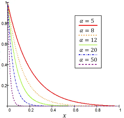
, (2.4)
is 1 in the range of interest, and intersects the abscissa at 1 (Figure 2.1).
Figure 2.1 Equation (2.4) for five different values of . In Algorithm 2.2, ∈ , is a random number
and , is multiplied by the distance to a design vector boundary.
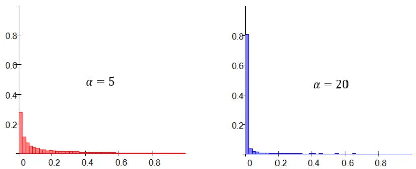
Figure 2.2 Histograms indicating distributions for the output of (2.4) given 10000 randomly generated
∈ , . a. . b. .
2.2.2 The Cost-Sorted Distance Method
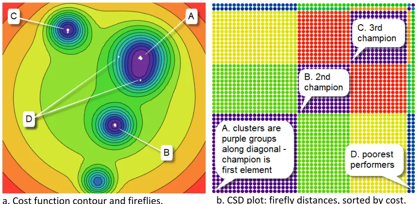
a. Cost function contour and fireflies. b. CSD plot: firefly distances, sorted by cost.
Figure 2.3 a. A typical 2D cost function contour plot with fireflies (white data points) in their final
migration positions – fireflies have clustered near three local minima; b. CSD plot : distances between
normalized fireflies, arranged in order of cost. Clusters of fireflies appear as blocks of uniform color;
their relative performance corresponds to distance from the origin.
plot indicates the likely presence of local minima. This ability to clearly display clusters of results and their champions is a significant benefit for designers dealing with high order problems (3D and higher), where cost functions can be difficult or impossible to visualize graphically.
2.2.3 Identifying CSD Cluster Champions
The CSD method is automated in step 5.4 of Algorithm 2.1, where local champions are extracted from clusters of fireflies. If desired, variations of these champions may replace the population’s lowest cost members after a subset of firefly migrations – this could accelerate convergence toward identified minima at the expense of reducing the scope of the search. For the examples discussed later in this chapter, replacement of the highest-cost fireflies is enabled for migrations ⁄3, and the replacement fireflies are randomly distributed within 1% of the distance between the champion’s elements and those of the lower or upper bounds.
a. CSD plot, vertical projection b. CSD plot w/ first row lines c. CSD first row w/ champions
Figure 2.4 CSD plot views : a. The typical vertical projection. b. A rotated view shows the planes of similar
distance distributed along the vertical axis. Black lines connect the first row data points – these are
distances from the lowest cost firefly to the others. c. A scatter plot of just the first row data; champions
indicated by red boxes.
Algorithm 2.3 The histogram approach used in step 5.4.1 of Algorithm 2.1 to identify cluster champions.
2.2.4 Configurable Benchmark Function
Numerous benchmark functions for optimization algorithm evaluation and development have been documented [7], [11]. A special type is required for assessing an algorithm’s capability to find alternative solutions to the global minimum. A parametric, multi-degree-of-freedom, multimodal benchmark function (2.5) is introduced for this purpose:
, , , , , , 1 0.5 1 〈 〉 . (2.5)
This is an n-dimensional (nD) spherical basis function multiplied by nD exponential functions for generating local minima. Vectors and are 1 factors for specifying depth and breadth, respectively, of local minima, is an array of minimum locations (seeds), and is a scalar that affects the shape of the spherical basis function.
1. Given a set of cost-sorted fireflies , and a maximum number of histogram bins :
2. Compute the CSD matrix: , ← | |, for all combinations , of fireflies.
3. Compute the maximum distance between fireflies ← / .
4. The lowest cost firefly is always the first champion: ∗ ← .
5. WHILE bins recorded is less than and there are still unprocessed fireflies,
5.1. Extract the first column of the CSD matrix: ← 〈 〉.
5.2. FOR 1, 2, … , , remove fireflies in the current bin:
5.2.1. IF , eliminate .
5.3. Record the champion of the next bin: ∗ ← .
5.4. Compute the CSD matrix: , ← | |, for all remaining fireflies , .
Some notable properties of (2.5) include: the basis function has a minimum value of 1.0 at 0.5 for 1, 2, … , corresponding to the center of the design space (without loss of generality, since design variables are to be normalized 0, 1 ); locations of local minima, neglecting cross-effects, are specified by where , ∈ 0, 1 for 1, 2, … ; function values at those locations,
neglecting cross-effects, are specified by 1 where ∈ 0, 1; for 0, the lowest possible minimum value at any point is 0; breadth of the local minima is dictated by , where larger values make them more narrowly focused (in the cases explored, ∈ 10, 250). The parametric nature of (2.5) enables programmatic generation of nD cost functions with specified (randomly if desired) shape and seed locations.
a.
b.
c.
Figure 2.5 Examples of a. 1D, b. 2D, and c. 3D cost functions from (2.5) with randomly generated
parameters. The number of seeds is for each of these, where is the degrees of freedom. Seeds, shown
in red, were randomly generated within prescribed subsections of the design space to prevent overlapping
minima. Cost is indicated by density of the points in the 3D case; darker is lower.
Seeds, shown in red, were randomly generated within prescribed subsections of the design space to prevent substantially overlapping minima.
2.2.5 FA Parameter Tuning
While the FA method is capable of identifying local minima, tuning its parameters to reliably do so can be challenging. A configurable benchmark function may be used as part of an optimization process (Procedure 2.1) to tune FA parameters for prototypical optimization problems. The prototypical problem is represented by (2.5) with parameters , , , , , and chosen randomly from a predetermined range as in Figure 2.5. Optimization using Algorithm 2.1 with FA parameter set , , , , and is performed and its result assessed. Results for different FA parameter sets are compared and the most reliably effective tuning set is chosen.
Procedure 2.1 Tuning FA parameters for a broad class of optimization problems. Statistical methods
are employed because the FA and the prototypical problem with randomized parameters (2.5) are
stochastic. The resulting tuning is desirable in the sense that it minimizes the cost function described in
Algorithm 2.4.
Step 1 of Procedure 2.1 requires assessment of FA tuning. Algorithm 2.4 is designed for this; _ , , where is an arbitrary instance of (2.5), its parameters , , and c randomly 1. Develop a cost function _ to assess the fitness of given firefly population for indicating
multiple minima of typical parametric benchmark functions. i.e. ideally, each firefly should be
near a local minimum; multiple local minima should have been found; etc. This cost will be
associated with a given FA tuning parameter set.
2. Choose a representative FA tuning parameter set – e.g. the designer’s best guess at good tuning.
3. Determine the number of evaluations required to achieve repeatable results (results are stochastic
and must be averaged):
3.1. FOR 10, 25, 50, 100, 250, 500, 750, 1000 (for example)
3.1.1. FOR 1, 2, . . , (e.g. 25)
3.1.1.1. Compute the mean _ from optimizations of randomly generated
benchmark problems using the representative FA tuning parameter set:
_ ← _
3.1.2. Compute the average and standard deviation of _ .
←∑ _ _
← _
4. Analyze and . Choose ∗ as small as possible but so that is repeatable
for a given FA parameter tuning set. Consider for comparison, associated with a random
(initial, prior to optimization) firefly population.
5. Select a range for each FA tuning parameter and perform a full factorial search for the best tuning
set – that which achieves minimum ∗ .
5.1. For each FA tuning set:
5.1.1. Perform ∗ optimizations of randomly generated benchmark problems.
5.1.2. Record ∗ .
generated each time it is called, and the set of final firefly locations. Tuning parameters that minimize _ provide the highest likelihood that fireflies will migrate to multiple minima for problems of the type (2.5), and provide a basis for choosing initial tuning for generic problems of similar complexity. It should be emphasized that FA and (2.5) with randomly generated parameters are stochastic; therefore, _ for a given tuning parameter set is averaged over multiple runs to minimize the effects of variation (steps 1 through 4 of Procedure 2.1 involve determining a sufficient number of runs). A full factorial optimization (as specified in Procedure 2.1, step 5) or other robust method may be employed in finding tuning parameters that minimize Algorithm 2.4 most reliably.
Algorithm 2.4 A function for quantifying the extent to which a set of design vectors have converged near
the seeds of the function . Returned is a sum of the average distance from each design vector to its
closest seed location, the average distance from each of a subset of minima to its nearest design vector, and
the difference between the cost function of the best design vector and the global minimum. Firefly tuning
is sought which minimizes this cost function.
The FA (Algorithm 2.1) was tuned using Procedure 2.1. The cost associated with each tuning parameter set was averaged from multiple optimizations of randomized 4D benchmark problems, these being a proxy for typical optimization problems. Four FA parameters
of Algorithm 2.1 were tuned (others were prescribed: 50, 50, and _ , , :
1. Given normalized, cost-sorted D design vectors and a scalar cost function with
cost-sorted D seed locations , assess the extent to which design vectors have converged upon ’s
minima:
2. FOR 1, 2, … ,
2.1.1. ← distance from to the nearest min location
3. FOR 1, 2, … ,
3.1.1. ← distance from to the nearest design vector
4. ← subset of the best few elements of , if desired
1) by selecting those from a full factorial search that minimize Algorithm 2.4 (i.e. _ , … where is the 4D benchmark problem (2.5) with parameters randomly generated each time it is called). Nine values of each tunable FA parameter were considered in the search, from 10 to 50, for a total of 9 6561 FA parameter sets. The parameter set with the lowest
_ is used for subsequent optimizations.
Figure 2.6 Averages and standard deviations from 25 batches of _ as functions of the number of
optimizations in each batch for fixed FA tuning parameters : . a.
The means, indicated by circles, with one standard-deviation bands extending above and below. b. The
standard deviations of batches of the averages as a function of the number of FA evaluations in each batch.
With 500 FA optimizations (circled in red), the average cost for these FA parameters is 0.57 and the
standard deviation of the averages is 0.03.
Performing 500 sequential FA optimizations required 3 minutes on a desktop computer with a 2.7 GHz quad-core processor, translating to 14 days of sequential computing for the full factorial search. Table 2.1 shows the 10 lowest resulting cost FA parameter sets. Averages of
_ from 500 evaluations each of the 6561 FA parameter sets ranged from 0.469 to 1.434; in contrast, the average from 25 batches of 500 evaluations of initial firefly populations (a worst case
Table 2.1 The 10 lowest cost results from a full-factorial FA parameter search. For each of the 6561
parameter sets, an average cost was computed from 500 FA optimizations. Other FA parameters were
prescribed: , , and . The lowest cost set is
employed for results of the following sections.
set _
1 10 35 15 20 0.469
2 15 35 15 25 0.490
3 10 40 15 20 0.491
4 10 40 35 20 0.494
5 10 25 35 20 0.498
6 10 35 20 15 0.508
7 10 25 25 15 0.509
8 10 25 35 15 0.510
9 15 35 30 25 0.510
10 15 25 25 15 0.511
Benchmark Optimization: 1D, 2D, 3D, and 4D
Optimization of randomized benchmark functions (2.5) was conducted for 1D, 2D, 3D, and 4D problems. In all of these cases, FA parameters from the full factorial search resulting in lowest _ were employed: 50, 50, 10 35 4/ , 1 1 ,
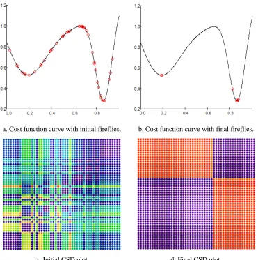
15 20 4/ . Note, and are multiplied by 4/ to scale the FA parameters (which were tuned using 4D benchmark problems) to the nD case. Computing each of these results required approximately 0.25 seconds on a desktop computer with a 2.7 GHz quad-core processor. Figure 2.7 shows a typical 1D result. The cost function was generated using (2.5) with: 2,
a. Cost function curve with initial fireflies. b. Cost function curve with final fireflies.
c. Initial CSD plot. d. Final CSD plot.
Figure 2.7 1D cost function (2.5) with initial and final firefly positions and corresponding CSD plots.
Fireflies are red data points in the cost curves.
population, clearly shows a bimodal result. The 1st and 33rd fireflies are obvious champions.
Note that the CSD plot does not indicate the relative cost of the two solutions, just that two have been found and one is better than the other.
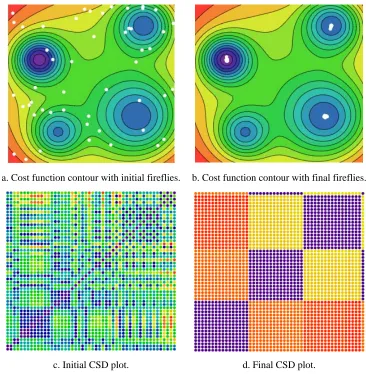
Figure 2.8 shows a typical 2D result. The cost function was generated using (2.5) with parameters: 4, 2, 0.89 0.68 0.64 0.58 , 55.7 34.7 17.9 48.6 ,
0.19
a. Cost function contour with initial fireflies. b. Cost function contour with final fireflies.
c. Initial CSD plot. d. Final CSD plot.
Figure 2.8 2D cost function (2.5) with initial and final firefly positions and corresponding CSD plots.
Fireflies are white data points in the contour plots.
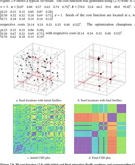
Figure 2.9 shows a typical 3D result. The cost function was generated using (2.5) with: 6, 3, 0.87 0.80 0.57 0.63 0.74 0.75 , 70.0 52.8 66.5 59.0 88.0 95.8 , 0.23 0.30 0.71 0.15 0.32 0.18 0.15 0.32 0.18 0.85 0.18 0.14 0.87 0.69 0.14 0.28 0.71 0.13 ,
1. Seeds of the cost function are located at , with
respective costs 0.14 0.24 0.32 0.35 0.48 0.52 . The optimization champions are 0.23 0.15 0.15
0.30 0.67 0.32 0.86 0.280.69 0.71
0.70 0.62 0.18 0.14 0.14 , with respective costs 0.14 0.24 0.32 0.48 0.52 .
a. Seed locations with initial fireflies. b. Seed locations with final fireflies.
c. Initial CSD plot. d. Final CSD plot.
Figure 2.9 3D cost function (2.5) with initial and final migration firefly positions and corresponding CSD
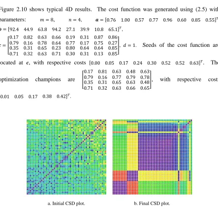
Figure 2.9.c shows a less ordered initial population compared to the previous two figures because the design space is larger relative to the number of fireflies. Figure 2.9.d clearly indicates 5 distinct clusters within the final firefly population (blocks of dark blue data points). Comparing this to Figure 2.9.c, the found clusters are near 5 of the 6 cost function seeds. Figure 2.10 shows typical 4D results. The cost function was generated using (2.5) with parameters: 8, 4, 0.76 1.00 0.57 0.77 0.96 0.60 0.85 0.55 ,
92.4 44.9 63.8 94.2 27.1 39.9 10.8 65.1 , 0.17 0.79 0.35 0.71 0.82 0.16 0.31 0.32 0.63 0.78 0.65 0.63 0.66 0.64 0.23 0.71 0.19 0.77 0.80 0.30 0.31 0.17 0.64 0.31 0.87 0.75 0.64 0.13 0.86 0.27 0.85 0.85
, 1. Seeds of the cost function are located at , with respective costs 0.00 0.05 0.17 0.24 0.30 0.52 0.52 0.63 . The optimization champions are
0.17 0.79 0.35 0.71 0.81 0.16 0.31 0.32 0.63 0.77 0.65 0.63 0.48 0.79 0.63 0.66 0.63 0.78 0.48 0.65
, with respective costs 0.01 0.05 0.17 0.38 0.42 .
a. Initial CSD plot. b. Final CSD plot.
The 4D cost function and firefly locations are not easily plotted in Figure 2.10 as they were for the 1D through 3D problems. The initial and final CSD plots, though, are shown and provide the same useful information about their respective populations. Three clusters of fireflies are apparent in Figure 2.10.b, and their champions are near the three lowest cost seeds.
Table 2.2 shows a statistical summary of results from application of Algorithm 2.1 for 1000 each of 1D, 2D, 3D, and 4D randomized benchmark optimizations. Both of two minima were found (i.e. a champion was within 1% of a seed or had a lower objective function value than the nearest seed) by the optimizer in 85% of 1D runs – one of two minima was found in 15% of runs. Two or more of four minima were found in 100% of 2D runs. The mode of minima found was 4 and the average was 3.65. Two or more of 6 minima were found in 93% of 3D runs. The mode of minima found was 4 and the average was 3.97. Two or more of 8 minima were found in 89% of 4D runs. The mode of minima found was 4 and the average was 3.57. At least one minimum was found by the optimizer in all runs.
Table 2.2 Summary of 1D-4D benchmark optimization results. Optimization was completed for 1000 each
of 1D, 2D, 3D, and 4D randomized benchmark problems. The first measure is the percentage of runs
where multiple minima were found. The number of minima found (mode and mean) for those runs is also
shown. Mode and mean are not shown for the 1D problem because in all cases where multiple minima
were detected, two were detected (there were always exactly two).
measure 1D 2D 3D 4D
2.3
Example: Electromechanical Design
Optimization
2.3.1 Active Magnetic Bearing and Controller
Typically in the design of electromechanical devices, the hardware and control algorithms are designed separately. A more satisfactory solution may be realized by parameterizing and optimizing these tasks simultaneously. The electromechanical system shown in Figure 2.11 is an active magnetic bearing (AMB), where voltage is manipulated to produce electromagnetic forces that maintain a desirable separation (levitation) between the shaft and electromagnet poles. Shaft displacement is sensed and fed back to a control algorithm, in this case a proportional + integral + derivative (PID) controller with gains ( , and , respectively) that must be optimized for stability and performance. The coil length , outside diameter , and wire gage must also be specified. The 6D design vector is therefore
Figure 2.11 Schematic of a longitudinal AMB, where the separation between stator and mover is
maintained by a PID controlled coil voltage. The shaft and electromagnet core are made of electrical steel
with relative permeability and mass density . . The shaft diameter is ,
the shaft length is , and the ferrous portion of the magnetic flux path, labeled , also has length
. One-dimensional motion is assumed.
Assessing performance requires a dynamic model of the system, parametric in terms of the design variables. Such a model, a coupled set of nonlinear ordinary differential equations (ODEs) derived from physical laws, is fully developed in the appendix (A.25):
2
L 2
2
L 2
, (2.6)
resistance. The many parameters of (2.6) are reduced to a set of three through the geometry of Figure 2.11 and relationships detailed in the appendix.
The PID control voltage is
⋅ ⋅ ⋅ (2.7)
where is the displacement error and is the desired displacement. A disturbance force such as (2.8) may be used to evaluate the system’s robustness:
Φ Φ ⋅ 1 sin (2.8)
where 5 and /2 are disturbance amplitudes, Φ is the Heaviside step function, 1/3 , 2/3 , and 10 is a disturbance frequency. While the choice of disturbance force profile is somewhat arbitrary, the designer must ensure a physical limitation that net force remains positive; electromechanical forces of this type (reluctance forces) are exclusively attractive.
Stability and performance of this AMB system can be quantified using a penalty function
0, (2.9)
where
max | | , (2.10)
, (2.11)
2.3.2
FA
Optimization
of
AMB+PID
Design
Parameters
The 6D engineering design (AMB with PID control) cost function (2.9) was optimized using Algorithm 2.1 with the FA tuning resulting from Procedure 2.1 ( 50, 50,
10 35 4/ , 1 1 , 15 20 4/ , 6 ). The system of equations (2.6) was simulated using an Adams-Bashforth ODE solver with convergence tolerance 0.001. Computing this result required approximately 18 minutes for a computer with a 2.7 GHz quad-core processor.
Figure 2.12.a and b show initial and final CSD plots for the AMB design example. Figure 2.12.c shows the design champions identified using Algorithm 2.3.
a. Initial CSD plot. b. Final CSD plot. 26 12.9 16.4 79824 720211 883 26 13.0 16.4 79415 372362 896 26 13.0 16.3 78904 246117 855 26 11.3 18.6 49058 703236 627 28 10.8 12.9 89356 729545 674 c. Optimization result: champions.
Figure 2.12 AMB design example with initial and final CSD plots and designs resulting from firefly
While the resulting CSD plot (Figure 2.12.c) is not as simple as those associated with benchmark problems (this is not an atypical plot for larger problems), there is still evidence of firefly clustering and there are some clear candidates for further investigation. The first 10 fireflies (the lowest cost grouping, dark blue in the bottom left corner of the plot) are relatively near one another. The second cluster begins with firefly 11 and ends with firefly 23; a third cluster comprising fireflies 18, 19, and 21 are intermingled with these. The fourth cluster begins with firefly 24 and ends with firefly 39. Fireflies 26 and 41 are the fifth cluster.
Table 2.3 lists the design parameters and other pertinent results for each identified AMB design champion.
Table 2.3 FA optimization champions and associated of the engineering design example.
value symbol units
wire gauge ‐ 26 26 26 26 28
coil diameter 12.9 13.0 13.0 11.3 10.8
coil length 16.4 16.4 16.3 18.6 12.9
proportional gain / 79824 79415 78904 49058 89356
integral gain / 720211 372362 246117 703236 729545
derivative gain / 883 896 855 627 674
resistance Ω 4.39 4.43 4.44 3.61 5.61
coil loops ‐ 597 600 600 539 544
max. acceleration max | | / 79.8 78.2 80.1 76.4 78.3
average power / 4.60 4.62 4.65 4.65 7.08
max. flux density 0.32 0.32 0.32 0.33 0.30
cost ‐ 6118 6203 6314 6343 6638
the designs achieve maximum magnetic flux density well within the required limit. The average power consumption is similar between the first 4 designs, and is somewhat higher for design 5.
Figure 2.13 shows the transient responses associated with these designs. It should be noted that the initial displacement error is -1mm, an impulse is applied at , and a sinusoidal disturbance is applied at . All five designs exhibit stable AMB control; their responses appear similar in Figure 2.13.a (the full 2mm scale), and are similar enough that transient response does not seem a significant differentiator in the design choice. Small differences in response are apparent in Figure 2.13.b (the 0.2mm scale). Design 2 has the smallest initial overshoot; Design 4 has the largest. Design 1 has the smallest response to the step in disturbance force at ; Design 4 has the fastest recovery from it; Design 3 has the slowest. Compared to the others, Designs 4 and 5 have similarly higher amplitude responses to the oscillatory disturbance initiated at .
a. ordinate scaled from -1 to 1 mm b. ordinate scaled from -0.15 to 0.15 mm
Figure 2.13 Transient simulation results (error: (mm) vs. time: t (s) for the AMB FA
optimization champions. The plots show identical data, but plot a is scaled to show the full scale and plot
2.4
Discussion/Conclusions
The improved FA (Algorithm 2.1) has been demonstrated capable of accurately finding multiple solutions (i.e. design alternatives) for 1D through 4D benchmark problems and of finding multiple satisfactory designs for a practical engineering problem. Procedure 2.1, a method to find good FA tuning using Algorithm 2.4 and the randomized 4D benchmark problem has also been demonstrated. The resulting tuning was shown to work well for all the problems explored.
FA tuning resulting from application of Procedure 2.1 worked well for finding multiple accurate solutions of 1D, 2D, 3D, and 4D benchmark problems even though it was derived using the 4D problem. Individual examples of optimization results were given for 1D-4D benchmark problems. Both minima were found (meaning a champion was within 1% of a seed or had lower cost) for the 1D problem; the best 3 of 4 for the 2D problem; the best 3 and 5 out of 6 for the 3D problem; and the best 3 of 8 for the 4D problem. A summary of results was presented in Table 2.2 for optimization of 1000 each of 1D, 2D, 3D, and 4D randomized benchmark problems. In these optimizations, two minima were found for 85% of 1D problems, two or more were found for 100% of 2D problems, 93% of 3D problems, and 89% of 4D problems. At least one minimum was always found.
Many of the methods developed (those summarized in Procedure 2.1) provide a basis for systematically finding optimal FA parameters for typical problems – a need identified in the literature [12]. This is not meant to imply that it is difficult to find reasonably good tuning for Algorithm 2.1. Accurate results were produced using the optimal FA tuning, but many other tuning sets would likely give similarly accurate results. The range noted of _ averages (0.47 to 1.43 for the full factorial search) is not large considering that there are 6561 tuning sets and a random firefly population achieves _ 7.26 on average, with standard deviation
The CSD method for identifying champions of clustered design populations was introduced. It is naturally compatible with FA and was incorporated in Algorithm 2.1. Interpretation of a CSD plot was demonstrated for a 2D problem by comparison to a contour plot showing the firefly locations overlaid with the cost function. This visualization method is more valuable for higher dimension problems where visualization by other means is difficult, as was demonstrated for 3D, 4D and 6D problems. The useful character of the CSD plot (the blocked or plaid appearance with champions near local minima) is highly dependent upon the ability of an optimization algorithm to produce clusters near local minima of the cost function. FA was shown to be capable of producing clustered populations and Algorithm 2.1 was successfully optimized using Algorithm 2.4 to do so.
Chapter 3
Robustness Considerations
Associated with Firefly and the
Cost-Sorted Distance Method
3.1
Introduction
A modified firefly algorithm (FA) was demonstrated in Chapter 2 for optimizing nonlinear multimodal systems with multiple degrees of freedom. The algorithm was tuned to produce results clustered near multiple minima of the objective function. The cost-sorted distance (CSD) method, a tool for exploring the design space, was shown to clearly indicate clusters of designs and their relative performance so that the most attractive design alternatives may be easily found.
methods are suitable for achieving this characteristic. The purpose of this chapter is to examine whether the tools developed in Chapter 2 are useful in this regard.
Robust design optimization (RDO), i.e. methods for development of designs optimally insensitive to uncertainty [20], has been summarized by several authors in recent years. Notably, Beyer et al. [20] in 2007 provided a comprehensive survey of the field including classification of uncertainty types and appropriate methodologies for each of them. Extensive treatment was given to evolutionary algorithms in the context of robustness. Park et al. [21] in 2006 published an overview of robust design including definitions of key terms and concepts with thorough discussion of the Taguchi method of robust design. Jin et al. [22] in 2005 published a concise summary of evolutionary optimization methods for addressing uncertainty in the fitness function and design variables. Lelièvre et al. [23] in 2016 categorized methods by suitability for addressing objective function and/or constraint uncertainties and demonstrated development of appropriate objective functions.
Robust objective functions differ from their deterministic counterparts by incorporation of robustness measures. Beyer et al. described five types of robustness measures for design optimization. These are robust regularization, which involves finding the “worst case” objective function value associated with a range of design space; expectancy measures such as mean and standard deviation of the objective function for each design; probabilistic threshold
measures of robustness, i.e. the probability that the objective function will achieve some result for a given design; statistical feasibility with regard to constraint satisfaction; and possibilistic uncertainties that can incorporate subjective assessment [20]. Two types are considered in this work. They are expectancy measures (mean and standard deviation - the most widely encountered robustness measures [26]), and a probabilistic threshold measure called probability of dominance [27] (PoD).
RDO can be computationally prohibitive compared to deterministic optimization because robustness measures must be estimated for all evaluated designs. Monte Carlo analysis is often the most direct and reliable method for estimating a given design’s robustness [20]. This requires computing for a large number of neighboring designs and is likely to increase the number of function evaluations by orders of magnitude. Alternative approaches may be available depending on the problem type; these include estimates based on Taylor series expansion (robustness measures from analytically or numerically estimated local function expansions), and meta-model approaches (including Taguchi robust design, neural networks, kriging, etc.) where robustness measures are estimated from a surrogate function that is fit using a strategic few local design points. Meta model approaches are particularly useful when objective function evaluation is very difficult (if a physical experiment is required, for example). In this work (although deterministic measures derived by Taylor series expansion are demonstrated) the standard basis of comparison is Monte Carlo analysis
The hypothesis tested in this chapter is that the percentage of fireflies (PFF) in clusters generated by Algorithm 2.1 (without modification) reliably indicates the relative robustness of associated designs. The procedure is to empirically assess the degree of linear correlation between PFF and traditional robustness measures for optimizations of randomized parametric benchmark problems (2.5).
3.2
Methods
for
Quantifying
Robustness
The robustness measures considered here are expectancy measures (mean and standard deviation), and probability of dominance, i.e. PoD. Evaluation of these measures is considered in this section.
3.2.1
A
Deterministic
Approach
Symbolic objective functions facilitate deterministic expectancy measures based on Taylor series expansion. The Taylor series of through second order terms is
Δ Δ 1
2 Δ Δ ⋯ . (3.1)
It is important to include terms through at least second order to accurately estimate expectancy measures for functions with stationary points (e.g. minima). Assuming uncorrelated, zero-mean, normally distributed, random variables, the mean of (i.e. ) may be estimated [20]
≅ 1
2 , (3.2)
≅ 1
2 . (3.3)
This can be demonstrated with the simplest multimodal version of (2.4) (i.e. 2, 1):
1 0.5 1 〈 〉
. (3.4)
Applying (3.2) to (3.4), ,
≅ 1 0.5 1 〈 〉 1 〈 〉
2 2
〈 〉
1 〈 〉 1
2 〈 〉 〈 〉 1 0.5 1
2 〈 〉 〈 〉 1 0.5 1
〈 〉
2 2 〈 〉 〈 〉 1 0.5 1
〈 〉
2 2 〈 〉 〈 〉
1 0.5 1
2 〈 〉 2 2 〈 〉 2 1
2 〈 〉 2 2 〈 〉 2 1 〈 〉
1
2 〈 〉 〈 〉 2 2 〈 〉 2 2 〈 〉 0.5 1 .
(3.5)
,
≅ 2 1 〈 〉 1 〈 〉 1
2 〈 〉 2 2 〈 〉 〈 〉
1 0.5 1
〈 〉
2 2 〈 〉 〈 〉 1 0.5 1
2 2
〈 〉
1 〈 〉 1
2 〈 〉 〈 〉 1 0.5 1
2 〈 〉 〈 〉 1 0.5 1
〈 〉
2 2 〈 〉 〈 〉 1 0.5 1
〈 〉
2 2 〈 〉 〈 〉
1 0.5 1
2 〈 〉 2 2 〈 〉 2 1
2 〈 〉 2 2 〈 〉 2 1 〈 〉
1
2 〈 〉 〈 〉 2 2 〈 〉 2 2 〈 〉 0.5 1 .
(3.6)
If 0.2 0.5 , 100 500 , 0.15 0.75 , 1, then (3.4) is
1 0.5 1 0.2 . 1 0.5 . . (3.7)
Equation (3.7) is plotted in Figure 3.1. Its lowest minima are 0.8946 at 0.1624 and 0.5312 at 0.7495. The corresponding objective function and from (3.2) and (3.3), respectively (for normally distributed about and with 0.01) are
Figure 3.1 An example of the simplest possible multimodal objective function.
Clearly, (3.2) and (3.3) provide a way to directly evaluate these robustness measures, but they lead to large symbolic expressions for even relatively simple multimodal objective functions. Also, as dimensions and the number of minima increase, the complication apparent in these solutions increases exponentially. Partial derivatives can be numerically approximated to reduce the symbolic burden, but this reduces the approximation fidelity and can result in significant numerical expense as problem size grows. For large problems other methods are warranted.
3.2.2
Monte
Carlo
Approach
assumptions regarding input distributions. They do, however, require many cost function evaluations.
Computing and involves simply taking the average and standard deviation of a number of computer simulations:
≅ 1 ∆ , (3.8)
and
≅ 1 ∆ , (3.9)
where ∆ are samples from set of random numbers.
a. normally distributed inputs propagate to outputs b. histograms of the output distributions
Figure 3.2 Uncertainty propagation for each of two minima of a typical 1D benchmark function. The
function is evaluated at 10000 randomly selected points (normally distributed about each minimum), a.
The input distributions are identical with . . Normalized histograms of output distributions are
shown on the vertical axis. b. The output histograms are shown in closer detail.
The precision of Monte Carlo methods can be increased (until round-off due to floating point number representation becomes a limitation) by increasing the number of simulations. This is another advantage over Taylor series methods which require additional series terms to improve precision. The main advantage, though, is that it is negligibly more difficult to analyze any objective function using Monte Carlo than it is to analyze this simplest one.
3.2.3
Probability
of
Dominance
, ≅ 1 | , ∆ 〈 〉 , (3.10)
where ∆ ∈ , , is a vector of standard deviations corresponding to the rows of the set of proposed designs, ∈ , and
| , ∆ 〈 〉 1 ∆ 〈 〉 min.. ∆ 〈 〉
0 . (3.11)
The standard deviation of ∆ distribution is critical for PoD. If it is very small then the design with lowest will clearly dominate other designs. For example, in Figure 3.2 where 0.01, no perturbed designs associated with dominate any associated with (none of the black data points have lower than any of the red data points); so , 0.01 0 and
, 0.01 1. As grows in magnitude, some perturbations of are superior to those of . In Figure 3.3 where 0.025, the two output distributions overlap somewhat (in contrast to Figure 3.2 where they do not); here , 0.025 0.02230 and , 0.025 0.97770.
a. normally distributed inputs propagate to outputs b. histograms of the output distributions
Figure 3.3 Output distributions overlap somewhat for . (compare to Figure 3.2). The function
(3.7) is evaluated at 10000 randomly selected points (normally distributed about each minimum), a. The
input distributions are identical with . . Normalized histograms of output distributions are