Joint Analysis of Multiple Gene Expression Traits to Map Expression Quantitative Trait Loci

(1)

MAIA, JESSICA M. Joint Analysis of Multiple Gene Expression Traits to Map Expression Quantitative Trait Loci. (Under the direction of Professor Zhao-Bang Zeng).

The goal of this dissertation is to address the issue of how to meaningfully find

quan-titative trait loci (QTL) for correlated traits. It has been shown in the literature that a joint

QTL analysis of multiple traits can have more power and be more precise than single trait

QTL analysis when traits are correlated. Phenotypic correlation arises from environmental

correlation, genetic correlation, or both. We wish to characterize the extent of the genetic

correlation among traits.

First, we use a canonical transformation, in the form of principal component analysis,

to combine many correlated traits into one, and apply single trait QTL analysis to it. We

analyzed two different data sets: one from Saccharomyces cerevisiae, and another from

eucalyptus. The traits analyzed in both data sets were gene expression levels generated in

microarray experiments.

Subsequently, we implemented a novel multiple trait mapping method based on

Multi-ple Interval Mapping to functionally related clusters previously studied in Saccharomyces

cerevisiae. Treating RNA abundance as a phenotypic trait, we quantified the extent of

the phenotypic variance due to genetic variance, and found additional QTL, previously

undetected, which were functionally related to the clusters being studied.

The last part of our research contains a study of QTL for individual amino acid

biosyn-thetic pathways of Saccharomyces cerevisiae. In the first part of this chapter, we look at the

QTL topology for all individual amino acid biosynthetic pathways, finding a major

tran-scriptional regulatory region for traits in these pathways. In the second part, we look at the

QTL topology of some individual amino acid biosynthetic pathways in detail, paying close

(2)

by

Jessica Mendes Maia

A dissertation submitted to the Graduate Faculty of North Carolina State University

in partial fulfillment of the requirements for the Degree of

Doctor of Philosophy

Bioinformatics

Raleigh, North Carolina

2007

Approved By:

Dr. Trudy Mackay Dr. Jung-Ying Tzeng

Dr. Zhao-Bang Zeng Dr. Dahlia Nielsen

(3)

Dedication

(4)

Biography

Jessica Maia was born in Long Beach, California. She grew up in Brazil, in the small

historic town of Mariana, in the state of Minas Gerais. She has two younger brothers, Eric

(5)

Acknowledgements

I would like to thank my advisor, Dr. Zhao-Bang Zeng, and the members of my committee:

Dahlia Nielsen, Trudy MacKay, and Jung-Ying Tzeng for fruitful discussions and academic

(6)

List of Figures

Figure 1.1 Eucalyptus cross design. . . 10

Figure 2.1 QTL locations for all eucalyptus traits . . . 37

Figure 2.2 QTL locations for all eucalyptus genes . . . 55

Figure 2.3 QTL locations for principal components of all eucalyptus genes . . 56

Figure 2.4 QTL location for the first 12 principal components of all genes . . . 57

Figure 2.5 QTL locations for genes in cluster G2 . . . 58

Figure 2.9 QTL locations for principal components of cluster G3 . . . 62

Figure 2.12 QTL location for principal components of cluster G7 . . . 65

Figure 2.18 QTL location for principal component 6 of cluster G10 . . . 71

(11)

Figure 2.20 QTL location for principal component 7 of cluster G13 . . . 73

Figure 4.1 Distribution of QTL per chromosome . . . 121

Figure 4.2 Length and position of pathway QTL in chromosome III . . . 123

Figure 4.3 Phenotypic correlations . . . 131

Figure 4.4 Genetic correlations for pathway traits . . . 133

(12)

List of Tables

Table 1.1 Backcross QTL and marker genotype frequencies and effects . . . . 14

Table 1.2 QTL genotype probabilities given three marker genotype classes . . . 15

Table 1.3 QTL genotype probabilities given two marker genotype classes . . . 16

Table 2.1 Distribution of QTL for each eucalyptus cluster . . . 36

Table 2.2 Principal components per cluster with at least one QTL . . . 39

Table 2.3 Principal component QTL of traits with QTL located in a particular linkage group . . . 41

Table 2.4 Cluster B QTL location . . . 43

Table 2.5 Cluster E QTL location . . . 44

Table 2.6 Cluster F QTL location . . . 45

Table 2.7 Cluster H QTL location . . . 46

Table 3.1 Example: QTL positions . . . 85

Table 3.2 Example (continued): close linkage model . . . 86

Table 3.3 Example (continued): pleiotropic model . . . 86

Table 3.4 MIM effects - cluster E . . . 90

Table 3.5 MT-MIM cluster E initial model . . . 91

Table 3.6 Cluster E MT-MIM and MIM additive effects . . . 91

Table 3.7 Cluster E heritabilities . . . 92

(13)

Table 3.9 MT-MIM cluster G initial model . . . 95

Table 3.10 Cluster G MT-MIM and MIM additive effects . . . 95

Table 3.11 Cluster G heritabilities . . . 96

Table 3.12 MIM H cluster . . . 97

Table 3.13 Cluster H initial MT-MIM model . . . 98

Table 3.14 Cluster H - MT-MIM and MIM additive effects . . . 99

Table 3.15 Cluster H heritabilities . . . 100

Table 3.16 Cluster E genetic correlations . . . 111

Table 3.17 Cluster G genetic correlations - Part I . . . 112

Table 3.18 Cluster G genetic correlations - Part II . . . 112

Table 3.19 Cluster H genetic correlations - Part I . . . 113

Table 3.20 Cluster H genetic correlations - Part II . . . 114

Table 4.1 Distribution of QTL per pathway. . . 119

Table 4.2 Percentage and number of QTL per chromosome. . . 122

(14)

Chapter 1 Introduction

1.1 Foreword

Recently, quantitative trait locus analysis has been applied to microarray experiments,

treating RNA transcript abundance as a phenotypic trait (Brem et al., 2002; Yvert et al.

2003; Schadt et al. 2003; Kirst et al. 2005; Li et al. 2006). A quantitative trait locus (QTL)

for a gene expression trait is a regulatory region which has a polymorphism in the

segre-gating population. Expression QTL studies, which examine thousands of gene expression

levels, differ drastically from previous QTL studies which analyzed fewer number of traits.

The increase in the number of phenotypes presents new challenges to the realm of

quantitative trait locus mapping methods such as automating QTL software to perform

thousands of genotype vs. phenotype associations, and establishing QTL detecting

thresh-olds which take into account the multiplicity of hypothesis testing. In addition, groups of

(15)

into account when finding QTL for correlated traits.

This dissertation addresses the issue of finding quantitative trait loci for correlated gene

expression traits. It has been shown in the literature that a joint QTL analysis of multiple

traits can have more power and be more precise than single trait QTL analysis when traits

are correlated (Jiang and Zeng 1995; Knott and Haley 2000; Sorensen et al. 2003).

We approach the challenge of finding common expression QTL (eQTL) among traits in

two ways. First we find QTL for each expression trait individually, and scan the genome for

shared QTL among traits. Some of these shared QTL represent transcriptional regulatory

regions common to many traits. We then group gene expression levels which share a QTL

according to function or using cluster analysis. Given groups of related genes, most of

which share a QTL, we use a novel multiple trait QTL mapping method to estimate genetic

correlation among traits due the QTL they share.

Our second approach involves reducing the number of expression traits by dimension

reduction. We reduce the number of gene expression levels using principal components

analysis. We then apply single trait QTL mapping to these principal component traits,

hoping that the QTL we find for these principal components have similar location to QTL

which were found for each of the expression traits individually.

1.2 QTL Analysis Review

Using fine-scale molecular maps to find regions in the genome associated with a trait of

interest has been done successfully for many years (Lander and Botstein 1989; Haley and

Knott 1992; Jansen 1993; Zeng 1994). In this section, we review a few QTL studies and

some quantitative trait locus mapping methods, starting with the simplest method, which is

(16)

1.2.1 Genetic Maps

The goal of quantitative trait locus studies is to find regions of the genome associated

with a trait of interest. For these types of studies, measurements of the trait of interest

(phenotypic measurements) are needed as well as a genetic map.

Genetic maps show the order of markers on a chromosome, and the distance between

markers as a fraction of the recombination frequencies between them. One of the most

common mapping functions were introduced by Haldane (1919) and Kosambi (1944).

Hal-dane’s mapping function assumes that crossovers occur randomly and independently from

one another. Haldane’s mapping function is given by:

m=−ln(1−2c)

2 ,

wherecis the observed recombination frequency, andm is the map distance in Morgans. Kosambi’s mapping function allows for small interference and is given by:

m = 1 4ln

1 + 2c 1−2c

,

wheremandcare the same as in the Haldane’s mapping function.

1.2.2 QTL Studies

QTL studies have been done on a number of traits in different species such as bristle

number in Drosophila (Payne 1918; Thoday 1961), leanness in pigs (Smith and Bampton

1977), seed and pigment weight in beans (Sax 1923), heterosis in maize (Stuber et al.

1992), prolificacy in sheep (Pipe and Bindon 1982), among many others. The common

thread about these traditional QTL studies is that the number of traits being studied is

small.

More recently, QTL mapping methods have been used to find transcriptional regulatory

(17)

mapping has been applied to microarray experiments in order to better understand the

na-ture of regulatory regions of gene expression levels (Brem et al. 2002; Schadt et al. 2003;

Li et al. 2006). Using QTL mapping with mRNA abundance is treated as a phenotypic

trait, one can identify gene expression regulatory regions for each trait separately. This

allows for the study of patterns of cis vs. trans regulation in the entire data set (Yvert et al.

2003; Kirst et al. 2005).

Some expression QTL studies have a goal to better understand transcriptional

regula-tory regions. For example, Brem and colleagues (2002) and Yvert and colleagues (2003)

studied transcriptional regulatory patterns in yeast, revealing whether cis or trans

regula-tion is more prevalent. This issue is at the heart of whether transcripregula-tional regularegula-tion occurs

at the site of the gene whose RNA abundance is being studied (cis-regulation), or at some

other regulatory region (trans-regulation). Gibson and Weir (2005) discuss some

quantita-tive aspects of eQTL studies and summarize the extent of cis vs. trans regulation in various

experiments.

Other eQTL papers tie the eQTL regions found by analyzing gene expression levels, to

a phenotypic trait such as lignin biosynthesis in eucalyptus (Kirst et al. 2004), or fat pad

mass and obesity in mice (Schadt et al. 2003). For example, Kirst and colleagues (2004)

applied correlation analysis to each of the gene expression levels and diameter growth.

Some expression traits highly correlated with diameter growth also shared QTL with the

diameter growth trait.

Li et al. (2006) studied eQTL by environment interactions in C. elegans. RNA

abun-dance was measured in 80 samples at two different temperatures, at which there would be

differences in body size, lifespan and other characteristics. Li and collaborators (2006)

found that a significantly greater percentage of trans-acting genes showed eQTL by

envi-ronment interaction compared to cis-acting genes.

(18)

for eucalyptus and yeast, which are two data sets which will be studied further in this

dissertation.

1.2.3 Yeast Expression QTL Studies

The budding yeast data set which we used in our analysis was published in several

installments (Brem et al. 2002; Yvert et al. 2003; Brem and Kruglyak 2005). Each

installment expanded the number of segregants in the population. Subsequently, there have

been several studies which analyzed this same data set. Next we will describe the first two

papers which made the expression traits publicly available (Brem et al. 2002; Yvert et al.

2003) and some others which we find relevant.

Brem and colleagues (2002) studied transcriptional regulation in Saccharomyces

cere-visiae. Gene expression levels and marker genotypes were observed on two parental strains

and their progeny. The parental strains are from a laboratory strain (BY) and a wild strain

(RM). The progeny consists of 40 haploid samples.

Gene expression levels for 6,215 genes or expression traits were measured in the parental

strains with 6 replications. Twenty five percent of genes were differentially expressed

between the parental strains at a p-value < 0.005. These results were found using the Wilcoxon-Mann-Whitney test, permuting the data set to obtain a significance threshold.

Gene expression levels were also observed for 40 haploid progeny samples obtained

from the cross between the parental strains. Heritability for these expression traits was

computed for the progeny as a function of the ratio of the parental expression variance

to the segregant expression variance with the formula: (segregant variance - parent

vari-ance)/segregant variance. The expression traits were shown to have median heritability of

84%.

(19)

(2002) performed single marker analysis on 6,215 traits with 3,312 markers. A total of 570

expression traits showed associated with one or more markers with a p-value<5×10−5_.

Twenty percent of differentially expressed genes showed linkage to at least one marker

with a p-value<5×10−5_.

There are 262 gene expression traits which are linked to at least one marker in the

genome (p-value < 5× 10−5_{) which are not differentially expressed between parental}

strains (p-value<0.005). Brem and colleagues (2002) stipulate that these linkages could be false positives; or that in a given parent, many alleles with opposing effects regulate

gene expression, which would lower the expression difference between parents; or that

difference in expression levels between parents exists but there is lack of power to detect

QTL.

There are 1220 expression traits differentially expressed between parents (p-value <

0.005) which are not linked to any marker. Brem and colleagues (2002) argue that is

be-cause transcription is regulated by multiple loci, each with a small effect. For only about

20% of the genes differentially expressed is the single marker effect big enough to be

detected. Thirty-six percent of 570 traits with an eQTL are cis-regulated. Brem and

col-leagues define trait to be cis-regulated if the marker linked to it is within 10kb of that trait.

In the second yeast expression QTL paper published by the same group as Brem et al.

(2002), Yvert and colleagues (2003) expanded the initial data set, by increasing the number

of segregants in the cross to 86 samples. Yvert and colleagues (2003) found expression

QTL, using single marker analysis, for the expression of all genes in the yeast genome.

They found that 75% of all QTL were trans-acting QTL, and that most of these QTL were

not enriched for transcriptional factors.

In addition, Yvert and colleagues (2003) used hierarchical clustering to define gene

expression clusters. Yvert and colleagues (2003) focused on clusters in which gene

(20)

genes are expected to have pair wise correlation greater than 0.725 by chance. In

chap-ter 3, we re-analyze a subset of cluschap-ters shown in this paper, finding additional QTL and

genes under the QTL peaks which have similar functions to genes in a cluster. Yvert and

colleagues (2003) positionally cloned two trans-acting regulators; each regulator contains

a polymorphism and affects the transcription of functionally related genes in that cluster.

Brem and Kruglyak (2005) conclude that most QTL they detect for the yeast data set

they use have weak effects. The data set is the same as in Brem et al. (2002) and Yvert et al.

(2003), except that the number of segregants was increased to 112 samples and the number

of markers is 2,957. Single marker analysis was performed to detect QTL, and permutations

were used to declare QTL at 5% false discovery rate (Storey and Tibshirani 2003). Brem

and Kruglyak (2005) claim to find epistasis for about 16% of highly heritable transcripts

(h2 _>₀_.₆₈₇_{). The heritability of each transcript,}_h2_{, was computed as}_h2 _{= (}_σ2

s −σp2)/σ2p,

where σ2

p, σs2 are the pooled variance among parental measurements, and the phenotypic

variance among segregants.

Storey and collaborators (2005) used data from the same yeast experiment as Brem

and Kruglyak (2005) to come up with a new scheme to estimate epistasis between QTL.

Storey et al. (2005) performed QTL analysis of 6,216 yeast expression traits, using 3,312

markers and 112 haploid segregants. Storey et al. (2005) claim their sequential search is

more powerful to find main QTL effects and epistatic effects as compared to an exhaustive

2-dimentional scan.

The exhaustive 2-dimentional scan works the following way: for every expression trait,

every pair of markers is fitted to a model which includes two QTL main effects and an

epistatic effect. The model is:

expression= baseline level+locus1 effect + locus2 effect + epistatic effect + noise. (1.1)

In contrast with the 2-dimentional scan, Storey et al. (2005) used a sequential genome

(21)

are:

M0: expression=baseline level + noise

M1: expression=baseline level + locus1 + noise

M2: expression=baseline level + locus1 + locus2 + epistasis + noise.

In step one, one selects the QTL which shows the most improvement in the goodness of

fit of model M1 compared with model M0. Then Storey et al. (2005) select a second

QTL which is the one that shows the greatest improvement in the goodness of fit of M2

compared with model M1. A total of 170 QTL pairs were found to be significant under

model M2 at a false discovery rate of 10%.

Zou (2006) using the same data set, was able to find more gene expression traits which

had 2 QTL only but less epistatic interactions than Storey et al. (2005) by performing a

sequential genome scan slightly different than what is presented in Storey et al. (2005).

Zou’s method used Multiple Interval Mapping (Kao et al. 1999) on one expression trait at

a time. Zou’s strategy is as follows:

(1) search for the first QTL and add it into the model if its effect is significant at type I

error rate of 10%, obtained through permutations;

(2) if a QTL is found in step 1, add one QTL at a time into the model conditional on the

existing QTL in the model (given that the QTL effect is greater than the threshold);

(3) search for epistatic interactions between QTL found in steps 1 and 2;

(4) delete QTL from the model that are not significant at a type I error rate of 5%.

The main difference between the models of Zou (2006) and Storey et al. (2005) is

that Zou searches for epistatic interactions only after all the QTL main effects have been

added into the model. In addition, QTL are only added into the model if their effects are

significant. Surprisingly, the number of expression traits controlled by only 2 QTL at a false

discovery rate of 10% found by Zou is 729 compared with 170 of Storey et al. (2005).

(22)

trait locus analysis to genes expression levels of a eucalyptus inbred cross. The next section

describes some results for this data set.

1.2.4 Eucalyptus Expression QTL Studies

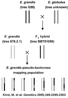
Kirst and colleagues (2005) studied transcriptional regulation of genes in an Eucalyptus

pseudobackcross: E. grandis × F1 hybrid (E. grandis × E. globulus). E. globulus has

high wood density and relatively slow growth; E. grandis has lower wood density but

faster growth. Crosses between these two strains have shown ample genetic and phenotypic

(23)

Kirst, M. et al. Genetics 2005;169:2295-2303

FIGURE 1.-- Mating design of the E. grandis pseudobackcross mapping population

Figure 1.1: Eucalyptus cross design.

Kirst and colleagues (2005) set out to discover the transcriptional regulation differences

between individuals in the same species and individuals in two related species. They used

the two marker maps to find expression QTL for 91 progeny samples. One map is that of the

F1 hybrid (tree BBT01058) and the other of the E. grandis backcross parent (tree 678.2.1)

(Figure 1.1). In the E.grandis marker map, there were a total of 96 AFLP fragments, in

12 major linkage groups; in the F1 hybrid map, there were a total of 122 fragments which

(24)

Of the 2,608 genes considered, 1373 (53%) were differentially expressed. Using

Com-posite interval mapping (Zeng 1994), Kirst and colleagues (2005) identified eQTL for 811

genes using the F1 hybrid map, and 451 eQTL using the E.grandis map. These eQTL were

significant using a type I error rate of 10% obtained through permutations.

Combining the eQTL data from both maps, 1067 traits had a total of 1655 eQTL. A total

of 821 gene expression traits had only one significant eQTL. Kirst and colleagues (2005)

estimated epistatic interaction via Multiple Interval Mapping (Kao et al. 1999). Epistatic

interactions were significant for 310 genes in the F1 hybrid map, and 285 genes in the E.

grandis map.

A total of 195 genes had eQTL in both marker maps, and 13 of these genes were located

in homologous regions. This suggests that most eQTL were trans-acting. Kirst et al. (2005)

argue that if cis-regulation were more prevalent, then we would see more homologous

eQTL. This result is the similar to yeast eQTL study of Yvert et al. (2003) which found

that trans-regulation is more prevalent than cis-regulation in yeast. Transcriptional hotspots

were found using both eucalyptus maps.

In another paper, Kirst et al. (2004) tied gene expression regulatory regions to regions

which regulate growth variation, previously detected by QTL mapping. The experimental

cross is the same one described previously in Kirst et al. (2005). QTL analysis for diameter

growth and for each of the 2,608 genes was done for 91 samples using Composite Interval

Mapping (Zeng 1993, 1994). Two significant QTL (experiment α = 0.01) for diameter growth were identified.

Subsequently, Kirst and colleagues (2004) applied correlation analysis to each of the

2,608 gene expression levels and diameter growth. A total of 37 gene expression levels

were correlated with growth (individual test significant threshold of 0.0001), most of which

were negatively correlated with diameter growth.

(25)

phenyl-propanoid pathways. High lignin content in a tree can be detrimental to growth (Kirst et

al. 2004). Then Kirst and colleagues (2004) confirmed that diameter growth and lignin

content were negatively correlated by sampling 8 individuals from the backcross progeny.

Kirst and colleagues (2004) also found common QTL for diameter growth and expression

levels of genes in lignin biosynthesis.

1.3 Review of Quantitative Trait Locus Analysis Methods

1.4 Single Trait QTL Mapping Methods

1.4.1 Single Marker Analysis

To find associations between a trait and a marker in a population, with marker classes

M/M,M/m, andm/mat a given loci, one can perform a parametric test such as thet-test or a non-parametric test such as the Wilcoxon-Mann-Whitney test. These tests can find

significant difference between trait means of different marker groups.

LetµM M,˜ µM m,˜ andµmm˜ be the observed trait means for individuals with marker geno-typesM/M, M/m, andm/mat a given locus respectively. And letnM M, nM m,andnmm

be the sample size of the marker classes, ands2

M M, s2M m, ands2mm be the sample variance

for each class.

Next we will give thetstatistic for a backcross and an F2population (Zeng 2000). For

(26)

additive marker effect is:

t = qµM M˜ −µmm˜ s2₍ 1

nM M +

1 nmm)

, where (1.2)

(1.3)

s = (nM M −1)s 2

M M+ (nmm−1)s2mm

nM M +nmm−2 . (1.4)

The test for dominance effect in the F2 population is:

t2 = ˜

µM m−µM M/˜ 2−µmm˜ /2 q

s2₍ 1 nM m +

1

4nM M +

1

4nmm)

, where (1.5)

(1.6)

s2 = (nM M−1)s 2

M M + (nM m−1)s2M m+ (nmm −1)s2mm nM M+nM m+nmm−3

. (1.7)

In a backcross population, there are only two marker classes, denoted here byM Mand

M m. The test statistic for a backcross population is:

t= qµ˜M M −µ˜M m s2₍ 1

nM m +

1 nM M)

, (1.8)

where

s2 = (nM M −1)s 2

M M+ (nM m−1)s2M m

nM M +nM m−2 . (1.9)

Single marker analysis for QTL mapping has been used for many years. Two problems

with single marker analysis are: it does not estimate QTL position and the difference in

trait means of marker classes is confounded with the recombination frequency between the

QTL and its flanking markers.

(27)

Table 1.1: Backcross QTL and marker genotype frequencies and effects (Zeng 2000)

QQ Qq

M M Frequency 1−r r

Effect µ+a µ+d

M m Frequency r 1−r

Effect µ+a µ+b

Below we will see how the difference in the trait means between marker classes in a

back-cross population is confounded by the recombination frequencyr:

µM M−µM m = [(1−r)(µ+a) +r(µ+d)]−r[(r(µ+a) + (1−r)(µ+d)](1.10)

= (1−2r)(a−d). (1.11)

Next we will find an improvement to single marker analysis, by a QTL mapping method

named interval mapping.

1.4.2 Interval Mapping

The precision of quantitative trait locus mapping methodology has increased

signifi-cantly since Lander and Botstein (1989) proposed Interval Mapping (IM), which can

esti-mate a QTL effect based on a marker map. Nonetheless, interval mapping was the

foun-dation for future QTL mapping methods, and the paper which introduced it (Lander and

Botstein 1989) was very influential.

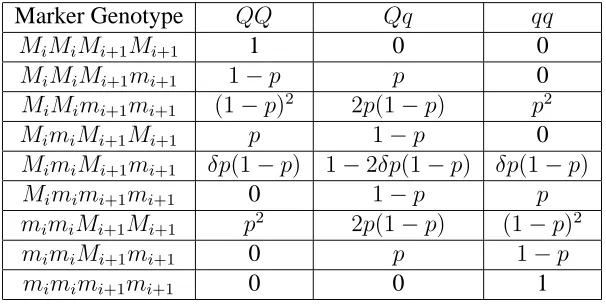
First, let’s establish the possible probabilities of a QTL genotype based on its flanking

marker genotypes. LetrMiQ be the recombination fraction between markerMi and QTL

Qand letrMiMi+1 be the recombination fraction between markersMi andMi+1. The next

(28)

population with three marker classes such as anF2population.

Table 1.2: QTL genotype probabilities given marker genotypes (Jiang and Zeng 1995)

Marker Genotype QQ Qq qq

MiMiMi+1Mi+1 1 0 0

MiMiMi+1mi+1 1−p p 0

MiMimi+1mi+1 (1−p)2 2p(1−p) p2

MimiMi+1Mi+1 p 1−p 0

MimiMi+1mi+1 δp(1−p) 1−2δp(1−p) δp(1−p)

Mimimi+1mi+1 0 1−p p

mimiMi+1Mi+1 p2 2p(1−p) (1−p)2

mimiMi+1mi+1 0 p 1−p

mimimi+1mi+1 0 0 1

wherep=rMiQ/rMiMi+1, andδ=r 2

MiMi+1/[(1−rMiMi+1)

2 ₊_r2

MiMi+1]. Double

recombi-nation is ignored.

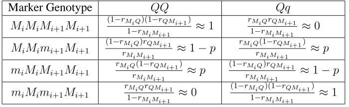
For a backcross population, the putative QTL genotype can take on two values,QQand

(29)

Table 1.3: QTL genotype probabilities given marker genotypes (Zeng 2000)

Marker Genotype QQ Qq

MiMiMi+1Mi+1

(1−r_MiQ)(1−r_QMi₊₁)

1−r_MiMi₊₁ ≈1

r_MiQr_QMi₊₁

1−r_MiMi₊₁ ≈0

MiMimi+1Mi+1

(1−r_MiQ)r_QMi₊₁

r_MiMi+1 ≈1−p

r_MiQ(1−r_QMi₊₁) r_MiMi+1 ≈p miMiMi+1Mi+1

r_MiQ(1−r_QMi₊₁) r_MiMi₊₁ ≈p

(1−r_MiQ)r_QMi₊₁

r_MiMi₊₁ ≈1−p miMimi+1Mi+1

r_MiQr_QMi₊₁

1−r_MiMi₊₁ ≈0

(1−r_MiQ)(1−r_QMi₊₁)

1−r_MiMi₊₁ ≈1

wherep=rMiQ/rMiMi+1.

For a backcross population, letyj be the phenotypic trait measurement for individuali;

bbe the effect of a single allele substitution at the QTL;x∗_{be an indicator random variable}

of the QTL genotype; b0 be the mean of the model, andej be a random variable which

follows a normal distribution N(0,σ2_{). Then interval mapping’s linear model is as follows:}

yj =b0+bx∗j +ej. (1.12)

The likelihood equation for interval mapping’s the linear model (equation 1.12) is:

L(b0, b, σ2) = n Y j=1

[Gj(0)Lj(0) +Gj(1)Lj]wherej = 1,· · · , n. (1.13)

The likelihood function is given byLj(x) = z((yj −(b0 +bx∗j)), σ2), where z(x, σ2) = (2πσ2₎−1/2_exp(₋_x2_/₂_σ2₎_{. The function} _G

j(x) represents the probability of the QTL

genotypexgiven the flanking marker genotypes (Table 1.3) . In the case of a backcross, the QTL genotypes QQ and Qq correspond to x values of 1 and 0 respectively. Lander and Botstein (1989) use the maximum likelihood analysis to obtain estimates of the model

parameters.

One disadvantage of interval mapping is that the additive effects estimated by interval

(30)

Zeng 1994; Kao et al. 1999). In addition, interval mapping is not an interval test, that is,

if there is a QTL, regions linked to it might appear to be significant even when there is no

QTL present in those locations (Zeng 1994).

1.4.3 Composite Interval Mapping

An improvement of the precision and estimates of QTL effects of Interval Mapping

came about when Jansen (1993) and Zeng (1994) independently used regression methods

which could take into account the presence of other QTL effects into a linear model.

Com-posite interval mapping (CIM), as labeled by Zeng (1994), used covariate markers to

esti-mate QTL position and additive effects. The linear model for composite interval mapping

is given by

yj =µ+b∗_x∗

j + X k6=i,i+1

bkxjk+ej, (1.14)

where:

yj is the trait value of thejth_individual, µis the mean of model,

b∗_{is the effect of the QTL expressed as a difference in effects between the homozygous}

and heterozygote QTL genotype classesQQandQq,

x∗

j is an indicator random variable taking value 0 or 1 with probability depending on the

genotypes of the flanking marker genotypes and the position of putative QTL (Table 1.3),

bkis the partial regression coefficient of the phenotypeyon thekth_{marker conditional}

on all other markers,

xjkis an indicator random variable for thejth_{individual and}_kth_{marker genotype which}

takes values 0 or 1 depending on whether the maker type is homozygote or heterozygote,

and

(31)

The known parameters arexjk, b0, yj. Using maximum likelihood analysis, the parameters b∗_{, bk, σ}2 _{are estimated.}

Composite interval mapping, unlike interval mapping, is an interval test. If linked

mark-ers to the QTL are included in the summation in equation 1.14, CIM is able to control for

the effects of other linked QTL in the model (Zeng 1993, 1994). In addition, if epistasis

is ignored, the partial regression coefficient bk, depends only on the QTL located in the marker interval being tested for the presence of a QTL (Zeng 1993, 1994).

The likelihood for a backcross population using composite interval mapping is:

L(b∗_{, B, σ}2_{) =} n Y j=1

[p1jφ(

yj −XjB−b∗

σ ) +p0jφ(

yj −XjB

σ )], (1.15)

whereXjB =µ+P

kbkxjk,

p1j is the probability that the markerx∗j is homozygous, and p0j is the probability that the markerx∗j is heterozygous.

Maximum likelihood analysis is used to find estimates for model parameters are computed

using the expectation maximization (EM) algorithm.

Defining a threshold to add or delete a QTL for this QTL mapping method is non-trivial

because the test statistic under the null hypothesis of no QTL is not known. A threshold

for QTL detection depends on the number of markers included into the linear regression

model, the size of the QTL interval being tested in terms of the genetic distance, and on

the sample size. In his 1994 paper, Zeng suggested that for a large sample size, and when

not too many markers are fitted into the model, that the value ofχ2

α/M,2 can be used as an

approximation for the100α%threshold value when there areM intervals in the genome in some marker scenarios.

Another way of finding an appropriate threshold to declare a QTL is to use

permuta-tions. Churchill and Doerge (1994) suggested simulating the null hypothesis of no QTL by

(32)

the maker genotypes for each individual fixed.

1.4.4 Multiple Interval Mapping

Kao et al. (1999) proposed a linear model which can fit multiple QTL into a model,

estimating both additive and epistatic effects of QTL which affect a given trait. They named

their model Multiple Interval Mapping (MIM). MIM can be more precise and powerful than

CIM.

The statistical backcross model for MIM (Kao et al. 1999) for traity, individuali, and

mQTL (Q1,· · · , Qm), can be written in the form:

yi =µ+ m X

r=1

arx∗_ir+ m X r6=k

δrk(wrkx∗_irx∗_ik) +εi, (1.16)

whereµis the mean of the model,

ar is the additive effect of QTLr,

x∗

ir represents the putative QTL genotype for individuali, QTLr, δrkis the indicator variable for epistasis between QTLrand QTLk,

wrkis the epistatic effect between QTLrand QTLk, and

εiis the error term for individuali, which we assume is distributed asN(0, σ2₎_.

The likelihood equation for MIM with a model nsamples, mQTL (Q1,· · · , Qm),

lo-cated in positions (p1,· · · , pm) forθ = (p1,· · · , pm, a1,· · · , am,· · · , wjk,· · · , σ2)is:

L(θ|X, Y) = n Y i=1 2m X j=1

pijφ((yi−µij)/σ), (1.17)

wherepij is a variable containing information about the probability of QTL genotypes. There are different ways of searching for QTL with MIM. One way is an iterative

(33)

effect, then tests for epistasis between QTL in the model. After that one would then re-test

QTL in the model for significance, and then optimize QTL positions. These steps would

be performed until no QTL can be added into the model according to a particular QTL

de-tection threshold or stopping criteria such as the information criteria (IC) (Stuart and Ord

1991; Miller 1990).

MIM has some advantages over other QTL mapping methods because unlike interval

mapping and composite interval mapping, with MIM epistatic interactions can be modeled

explicitly; MIM can also give better QTL position estimates because it searches

simultane-ously for QTL in multiple marker intervals.

1.5 Threshold for QTL detection

In classical QTL analysis, the number of traits analyzed is small compared to the

thou-sands and sometimes tens of thouthou-sands of traits analyzed in expression QTL studies. Even

though the statistical methodology of traditional QTL studies is used in the realm of eQTL

studies, figuring out significance levels for various QTL detecting methods is non-trivial.

One way of finding an appropriate threshold to declare a QTL is to use permutations.

Churchill and Doerge (1994) suggested simulating the null hypothesis of no QTL by

per-muting the trait values among individuals in the segregating population, while keeping the

maker genotypes for each individual fixed. One would then record the test values with the

permuted samples and compare them to test values obtained by applying a QTL mapping

method to the data of interest.

Zou et al. (2004) proposed a re-sampling method using the result that the score statistic

is asymptotically equivalent to the likelihood ratio statistic. This method has a much lower

computation burden than the permutation scheme proposed by Churchill and Doerge (1994)

(34)

In order to address this issue of testing many null hypotheses, Storey and Tibshirani

(2003) came up with an estimate of the positive false discovery rate (FDR). With this FDR

estimate, one can compute the expected proportion of genes which falsely were declared to

have one or more QTL, given the total number of expression traits with at least one QTL.

The FDR estimate of Storey and Tibshirani (2003) is applicable to eQTL studies where

thousands of QTL are claimed to be significant. Zou (2006) adapted Storey’s false

dis-covery rate methodology to multiple interval mapping (MIM). Model selection is an active

research area in QTL methodology development. Finding an appropriate threshold level

for which to add or delete QTL into a model is still very challenging.

1.6 Thesis chapters

In this first chapter, we described a few expression QTL studies, focusing on yeast and

eucalyptus expression QTL experiments. Then we reviewed a few QTL mapping methods

such as single marker analysis, interval mapping, composite interval mapping and multiple

interval mapping.

In the second chapter, we test the usefulness of principal component analysis in the

realm of QTL mapping. We transform the original traits using principal component

anal-ysis, and examine whether the QTL found for these principal component traits match the

location of QTL for individual traits. We analyzed two different data sets: one from

Sac-charomyces cerevisiae, and another from eucalyptus. The traits analyzed in both data sets

were gene expression levels generated in microarray experiments.

In the third chapter, we implement a novel multiple trait mapping method based on

mul-tiple interval mapping. We propose a way to find an initial model and to test for pleiotropy

vs. close linkage. We then apply this method to functionally related clusters previously

(35)

The fourth chapter is an analysis of transcriptional variation of gene expression levels

in yeast individual amino acid biosynthetic pathways. We look at the number of QTL

and the extent of pleiotropy in each pathway. We also estimate genetic correlations and

heritabilities for genes in individual amino acid biosynthetic pathways.

In this dissertation, we treated RNA abundance as a phenotypic trait for two

experi-mental crosses: one from eucalyptus and the other from yeast. Both crosses are modeled as

a backcross in the QTL experiment design. We analyzed a subset of Kirst and colleagues

(2005) eucalyptus data. We used their cDNA arrays consisting of 2,610 gene expression

levels measured on 88 samples of a eucalyptus pseudo-backcross: E. grandis x F1 hybrid

(see Figure 1.1). The average marker spacing is about 1 marker for every 10 centiMorgans.

The final version of the yeast data set we used was a subset of data set published in

Brem and Kruglyak (2005). This data set comes from a cross between a wild (BY) and

laboratory (RM) strains of Saccharomyces cerevisiae. The expressions of 6,195 genes

were measured in 112 haploid samples using a platform of custom open reading frames

(Yvert et al. 2003). In chapter 2, only 86 yeast samples were used which was the number

of available samples at that time. In chapters 3 and 4, 112 yeast samples are used in the

(36)

1.7 References

Brem, R.B., G. Yvert, R. Clinton and L. Kruglyak, 2002 Genetic Dissection of

Transcrip-tional Regulation in Budding Yeast. Science 296: 752-755.

Brem, R.B., and L. Kruglyak, 2005 The landscape of genetic complexity across 5,700 gene

expression traits in yeast. PNAS 102:1572-1577.

Churchill, G.A., and R.W. Doerge, 1994 Empirical threshold values for quantitative trait

mapping. Genetics 138: 963-71.

Gibson, G., and B. Weir, 2005 The quantitative genetics of transcription. Trends Genet.

21: 616-623.

Haldane, J.B.S., 1919 The combination of linkage values, and the calculation of distance

between the loci of linked factors. J. Genetics 8: 299-309.

Haley, C.S., and S.A. Knott, 1992 A simple regression method for mapping quantitative

trait loci in line crosses using flanking markers. Heredity 69: 315-24.

Jansen, R.C., 1993 Interval mapping of multiple quantitative trait loci. Genetics 135:

205-211.

Jiang, C., and Z.-B. Zeng, 1995 Multiple Trait Analysis of Genetic Mapping for

Quantita-tive Trait Loci. Genetics 140: 1111-1127.

Jiang, C., and Z.-B. Zeng, 1997 Mapping quantitative trait loci with dominant and missing

markers in various crosses from two inbred lines. Genetica 101: 47-58.

Kao, C.-H., Z.-B. Zeng and R. D. Teasdale, 1999 Multiple interval mapping for quantitative

(37)

Kirst, M., A.A. Myburg, J.P. De Leon, M.E. Kirst, J. Scott J, and R. Sederoff, 2004

Co-ordinated genetic regulation of growth and lignin revealed by quantitative trait locus

anal-ysis of cDNA microarray data in an interspecific backcross of eucalyptus. Plant Physiol.

135:2368-2378.

Kirst, M., C.J. Basten, A.A. Myburg, Z-B. Zeng and R.R. Sederoff, 2005 Genetic

Ar-chitecture of Transcript-Level Variation in Differentiating Xylem of a Eucalyptus hybrid.

Genetics 169: 2295-303.

Knott, S.A., and C.S. Haley, 2000 Multitrait least squares for quantitative trait loci

detec-tion. Genetics 156: 899-911.

Kosambi, D.D., 1944 The estimation of map distances from recombination values. Ann.

Eugen. 12: 172-175.

Lander, E.S., and D. Botstein, 1989 Mapping mendelian factors underlying quantitative

traits using RFLP linkage maps. Genetics 121: 185-99. Erratum in: Genetics 1994, 136:

705.

Li, Y., O.A. Alvarez, E.W. Gutteling, M. Tijsterman, J. Fu, et al., 2006 Mapping

deter-minants of gene expression plasticity by genetical genomics in C. elegans. PLoS Genet.

29:e222.

Miller, A.J., 1990 Subset Selection in Regression. Chapman and Hall, London.

Payne, F., 1918 The effect of artificial selection on bristle number in Drosophila

am-pelophila and its interpretation. Proc. Natl. Acad. Sci. U.S.A. 4: 55-58.

Piper, L.R., and R.M. Bindon, 1982 Genetic segregation for fecundidy in Booroola Merino

(38)

Congress on Sheep and Beef Cattle Breeding. Dunmore Press, Palmerston North,

Aus-tralia.

Sax, K., 1923 The association of size differences with seed-coat pattern and pigmentation

in Phaseolus vulgaris. Genetics 8:552-560.

Schadt, E.E., S.A. Monks, T.A. Drake, A.J. Lusis, N. Che, et al., 2003 Genetics of gene

expression surveyed in maize, mouse and man. Nature. 422: 269-270.

Smith, C., and P.R. Bampton, 1977 Inheritance of reaction to halothane anaesthesia in pigs.

Genet. Res. 29: 287-292.

Sorensen, P., M.S. Lund, B. Guldbrandtsen, J. Jensen and D. Sorensen, 2003 A comparison

of bivariate and univariate QTL mapping in livestock populations. Genet Sel Evol. 35:

605-622.

Storey, J.D., and R. Tibshirani, 2003 Statistical significance for genomewide studies. Proc.

Natl. Acad. Sci. U.S.A.100: 9440-9445.

Storey, J.D., Akey, J.M. and L. Kruglyak, 2005 Multiple locus linkage analysis of genomewide

expression in yeast. PLoS Biol. 3:e267.

Stuart, A., and J.K. Ord, 1991 Kendall’s Advanced Theory of Statistics. Oxford Univ.

Press, New York, 5th Ed., Vol. 2.

Stuber, C.W., S. E. Lincoln, D. W. Wolff, T. Helentjaris and E. S. Lander, 1992

Identifica-tion of Genetic Factors Contributing to Heterosis in a Hybrid From Two Elite Maize Inbred

Lines Using Molecular Markers. Genetics 132: 823-839.

(39)

Yvert, G., R.B. Brem, J. Whittle, J.M. Akey, E. Foss, et al., 2003 Trans-acting regulatory

variation in Saccharomyces cerevisiae and the role of transcription factors. Nat. Genet. 35:

57-64.

Zeng, Z.-B, 1993 Theoretical basis for separation of multiple linked gene effects in

map-ping quantitative trait loci. PNAS 90:10972-10976.

Zeng, Z.-B, 1994 Precision Mapping of Quantitative Trait Loci. Genetics 136: 1457-1468.

Zeng, Z.-B, 2000 Statistical Methods for Mapping Quantitative Trait Loci. Book manuscript.

Zou F, J.P. Fine, J. Hu, and D.Y. Lin., 2004 An efficient resampling method for assessing

genome-wide statistical significance in mapping quantitative trait Loci. Genetics

168:2307-2316.

Zou W., 2006 Transcriptional regulatory patterns in yeast revealed through expression

(40)

Chapter 2 Using Principal Component Analysis for

Expression Quantitative Trait Locus

Mapping

2.1 Abstract

In this chapter, principal component analysis is tested as a dimension reduction tool for

gene expression levels, which we consider as phenotypic traits for this study. We investigate

whether principal components can predict the patterns of association between genes and

the regions which regulate their expression. When principal components are used to take

(41)

component analysis is not a reliable tool to summarize gene expression levels because

QTL of principal components do not consistently map to the same regions where the QTL

of genes used to compute these principal components are located. However, the QTL

for the first principal component, whenever it exists, maps to the same location as the

QTL locations for genes used to compute the first principal component. We have tested

our methods on two micrroarray data sets. One from a eucalyptus pseudo-backcross and

another from a cross of wild and lab strain of Sacharomyces cerevisiae.

2.2 Introduction

Quantitative trait locus (QTL) mapping has been applied to microarray experiments in

order to better understand the nature of regulatory regions of gene expression levels (Brem

et al. 2002; Schadt et al. 2003; Li et al. 2006). Using QTL mapping with mRNA

abun-dance is treated as a phenotypic trait, one can identify gene expression regulatory regions

for each trait separately. This allows for the study of patters of cis vs. trans regulation in

the entire data set (Yvert et al. 2003; Kirst et al. 2005).

There are however, many reasons why one would want to apply QTL mapping to a

subset of the expression data or a transformation of it. One could apply QTL mapping only

to traits that are clustered together (Yvert et al. 2003), traits which have a related function

(Andersson-Eklund et al. 2000), or gene expression levels which share regulatory regions

(Brem et al. 2002). Principal component analysis (PCA) has also been used in the past

to summarize phenotypic measurements (Liu et al. 1996; Andersson-Eklund et al. 2000).

Here are some arguments why one would want to summarize a data set, or part of it, with

principal component analysis before QTL mapping:

(1) To capture a large amount of the variation with fewer variables. One could start

(42)

2000). Weller et al. (1996) suggested using PCA as a form of dimension reduction tool,

by finding QTL for principal components which capture a large percent of the variance,

and ignoring the principal components (PCs) that represent a “small percent of the total

variance”. Weller et al. (1996) use PCA to summarize three phenotypic traits related to

milk production in dairy cattle.

(2) To avoid issues of multiple testing. Finding a QTL for every trait in the dataset

can have less power to detect traits summarized by principal component QTL, because the

QTL mapping threshold has to be adjusted for the number of genotype-trait associations.

Therefore, if there are fewer principal components than traits in the data set, the number of

genotype-trait associations is smaller.

(3) To combine phenotypic measurements which together are indicative of complex

disease. Arguably, it makes sense to combine traits which are different measurements of

the same phenotype, and find QTL for the combined trait instead of each phenotypic

mea-surement separately. One example is osteochondrosis, a generalized skeletal disease in

pigs (Andersson-Eklund et al. 2000). In this study, eight bone density measurements were

combined by principal components; in a separate principal component analysis, four

os-teochondrosis scores from examination of lesions were combined as well. The correlation

between the bone density and osteochondrosis is small (Andersson-Eklund et al. 2000).

Both sets of traits (bone density and osteochondrosis measurements) were indicative of the

presence of osteochondrosis.

(4) To lessen the computational burden. Although the computation time for finding

associations between or thousands of genes and thousands of markers or marker intervals

takes a few days or less (Zou 2006), setting up scripts which automate the search for QTL

usually takes more time than performing the analysis itself, and requires knowledge of how

to write scripts which automate these tasks.

(43)

(Mahler et al. 2002; Andersson-Eklund et al 2000; Lan et al. 2003; Liu et al 1996).

What all of these studies have in common is the fact that principal component analysis is

applied to a small number of traits. The underlying assumption of these studies is that QTL

for traits to be summarized with PCA will be in close proximity to QTL of principal

com-ponents. The main goal of this report is to see if QTL for principal components can predict

QTL locations for individual traits (gene expression levels) that have a common function,

or that are clustered together, or both. Unlike other studies, this study looks at QTL patterns

for individual traits and for principal components in small and large trait clusters.

We treat RNA abundance as a phenotypic trait for two experimental crosses: one from

eucalyptus and the other from yeast. Both crosses are modeled as a backcross in the QTL

experiment design. In the first part of this report, we analyze the eucalyptus data set (Kirst

2004; Kirst et al. 2005). A two-way coupled clustering method is applied to the eucalyptus

gene expression levels. Then QTL analysis is applied to all traits in this data set.

Subse-quently, traits in each cluster which have one or more QTL are annotated. Then principal

component analysis and QTL mapping are performed on traits that are clustered together,

and on traits that have QTL located in common regions.

In the second part of this chapter, we compute principal components for yeast gene

expression levels clustered by Yvert et al. (2003). These clusters are composed mostly of

functionally related genes, which also have a high gene expression pair wise correlation.

We then find QTL for each trait in a cluster, and for the principal components of those

(44)

2.3 Materials and Methods

2.3.1 Expression Data Sets

We treated RNA abundance as a phenotypic trait for two experimental crosses: one

from eucalyptus and the other from yeast. Both crosses are modeled as a backcross in the

QTL experiment design. We analyzed a subset of Kirst and colleagues (2005) eucalyptus

data. We used their cDNA arrays consisting of 2,610 gene expression levels measured on

88 samples of a eucalyptus pseudo-backcross: E. grandis x F1 hybrid (E. grandis x E.

globulus). The average marker spacing is about 1 marker for every 10 centiMorgans.

The yeast data set we used was a subset of data published by Brem and Kruglyak

(2005). This data set comes from a cross between a wild (BY) and laboratory (RM) strains

of Saccharomyces cerevisiae. The expressions of 6,195 genes were measured in 86 haploid

samples using a platform of custom open reading frames (Yvert et al. 2003). The marker

density of this cross is on average one marker for every 3kb. There are a total of 2956

markers in this data set. The yeast microarray data was downloaded from Gene expression

Omnibus (Edgar et al. 2002), reference series: GSE1990.

2.3.2 Linkage map

The yeast linkage map was constructed using Mapmaker (Lincoln et al. 1992; Paterson

et al. 1988). The Saccharomyces cerevisiae genotypic data was obtained from direct

communication with Rachel Brem. The eucalyptus F1 hybrid paternal map (Kirst 2004;

Kirst et al. 2005) linkage map was obtained via personal communication with Matias

(45)

2.3.3 Principal component Analysis

Principal component analysis is a linear transformation of the data. For example,

imag-ine a data set with 88 samples and 2,610 gene expression levels. Each sample has a trait

measurement for each of the 2,610 traits. If one computes 12 principal components from

this data, each sample now will have only 12 trait measurements. The genotype information

for each sample remains unchanged.

Principal component 1 (PC1) captures a greater variance than any other; let v(PC(i)) be the variance in the data captured by principal component i. If there are k principal com-ponents in the data set, then v(PC(1))>v(PC(2)) >· · ·>v(PC(k)). Principal component analysis was done using proc princomp of SAS version 8.02 and JMP software.

2.3.4 Clustering Analysis

When applied to expression data, one-way clustering analyses assigns traits to groups

based on their similarity or dissimilarity. There are many types of clustering analyses

such as hierarchical methods (bottom-up and top-down methods), which yield nested sets

of clusters, and partitioning methods (K-means clustering, self organizing maps), which

assigns genes to a fixed number of clusters (Chipman et al. 2003).

Two-way clustering analysis seeks to cluster both samples and gene expression levels

at the same time. Two sets of gene expression levels might yield a different clustering of

the samples (Chipman et al. 2003). For the eucalyptus data set coupled two-way clustering

(CTWC) method was used to perform two-way clustering of the data (Getz et al. 2000).

This coupled two-way clustering method has been used in several studies (Alon et al. 1999;

Golub et al. 1999; Godard et al. 2003; Getz et al. 2003). The CTWC method uses subsets

of genes to cluster samples and vice-versa (Getz et al. 2000) because if one uses all traits to

(46)

other interesting clusters of samples (Chipman et al. 2003).

When applied to the eucalyptus data set, the CTWC method produced a total of 17 gene

expression clusters and 9 eucalyptus sample clusters. Four out of seventeen gene clusters

were excluded from the QTL analysis and principal component analysis because they had

972 or more traits, where the total number of traits is 2610. These four clusters were

excluded because they have at least 37% of all traits in the data set and are likely to contain

genes representing different biological processes. The clustering results were obtained by

uploading our data to an online server (Getz and Domany 2003).

For the Saccharomyces cerevisiae data set, we used four existing gene clusters for

prin-cipal component and QTL analysis. Yvert et al. (2003) clustered genes which are

function-ally related and/or have high phenotypic correlation (pair wise correlation>0.725). Genes in clusters B,E,F (discussed in section 2.5) have similar function and are highly correlated.

Functions of sixteen genes in cluster H are not known, although their gene expression levels

are highly correlated.

2.3.5 Gene annotation

Annotation for gene clusters was done using Blastx (Altschul et al. 1990), which

trans-lates a nucleotide query into a protein sequence, and searches for similarities among the

protein sequence of interest and all protein sequences in the database. The advanced

op-tions for the Blastx searches were set at default. The top three Blastx matches for each gene

in a cluster were considered if they had an E-value less than 1e-10. At an E-value of 1e-10,

“10 hits with scores equal to or better than the defined alignment score, S, are expected to

occur by chance (in a search of the database using a random query with similar length)”

(47)

Saccharomyces cerevisiae genes already clustered by Yvert et al. (2003) were used in

the PCA analysis. Out of the four clusters studied, genes in three of those clusters (B,E,and

F) are functionally related. Genes in cluster H have unknown function.

2.3.6 QTL Analysis

QTL mapping was done using the composite interval mapping (Zeng 1993, 1994)

func-tion of QTL cartographer (Wang et al. 2001-2004). For the yeast data set, we set individual

thresholds for QTL detection for each trait that was in one of the four clusters studied. The

5% type I error rate threshold for the yeast data was obtained using Windows QTL

Cartog-rapher with 500 permutations (Churchill and Doerge 1994) for each trait. The thresholds

we found were very similar to those of Zou (2006).

For the eucalyptus data set, we used QTL detection thresholds determined by Kirst

(2004). The empirical experiment wide threshold for type I error rate for QTL detection

using CIM at the 5%level, was determined to be a likelihood ratio (LR) greater than 12.0

(Kirst 2004). This empirical threshold was established using a permutation method

pro-posed by Churchill and Doerge (1994). Twenty genes were picked at random and five

hun-dred permutations were done for each gene. The 5%empirical threshold was determined

for each gene. The most stringent 5% threshold among the 20 genes was used. To

ob-tain a general picture of which regions regulate gene-expression, all eucalyptus traits were

mapped individually to regions in the genome using composite interval mapping (Zeng

(48)

2.4 Eucalyptus Results

2.4.1 Clustering and QTL Analyses

Table 2.1 shows the total number of traits in a cluster, and the number of traits which

(49)

Table 2.1: The first column of this table contains the cluster name; the second column has the number of traits in a cluster; the third column contains the number of traits which have at least one QTL, and the last column has the ratio of the cluster size and the number of traits which have at least one QTL.

Cluster Cluster Traits with Traits with at least 1 QTL/ Name Size at least 1 QTL Cluster Size

G3 276 26 .09

G7 248 32 .13

G8 166 46 .28

G2 124 41 .33

G10 72 2 .03

G4 64 1 .02

G13 62 18 .30

G9 60 16 .27

G16 46 3 .07

G6 44 6 .14

G5 36 4 .11

G15 26 8 .31

All Traits 2610 620 .24

There is an overlap of significant QTL between the clusters with 248 and 44 traits, and the

clusters with 248 and 36 traits. All the QTL of cluster with 44 traits are in cluster with 248

traits, and all the QTL of cluster with 36 traits are in the cluster with 248 traits. However,

the clusters with 44 and 36 traits do not have any QTL in common. A cluster with more

traits tends to have more QTL; however, the ratio of the number of QTL and the number of

traits per cluster does not seem to depend on the cluster size.

Kirst (2004) found that 811 traits with at least one QTL in the F1 hybrid paternal map

at type I error rate of 10%. We found that at a type I error rate of 5% (Kirst 2004), 620

(50)

see the next figure. Each trait was mapped individually using CIM (Zeng 1994). The figure

below shows a few QTL hotspots for all traits in the eucalyptus data set. These hotspots

are located around 0.5 M, 8.5 M, and 10 M. Similar results were obtained by Kirst et al.

(2005).

0 20 40 60 80 100 120 140 160

0 1 2 3 4 5 6 7 8 9 10 11 12

Number of QTLs (LR >12.0)

Position (M) All genes

Figure 2.1: QTL locations for all eucalyptus traits.

Graphs with the QTL locations for all clusters in Table 2.1 are in the Appendix. Next we

annotate each of these clusters to see if genes in them have a common function.

2.4.2 Eucalyptus Cluster Annotation

We annotated all traits in Table 2.1 which had at least one significant QTL, to see if

genes which are clustered together and share a QTL are functionally related. Annotation

(51)

Blastx matches for each trait in a cluster were considered if they had an E-value less than

1e-10. The clusters with 6 and 32 QTL (Table 2.1), have each two traits classified as

UDP-glucoses; the cluster with 46 QTL has two heat shock related proteins; the cluster

with 16 QTL has three traits in the dehydrogenase family. The cluster with 41 QTL has

three proteins classified as oxidoreductases, three as dehydrogenases, two as similar to

Arabidopsis thaliana transcription factors, and two classified as histones. Each of the six

remaining clusters did not have genes with a common putative function. Even though some

traits share the same QTL and are clustered together, they do not necessarily have the same

function.

2.4.3 Eucalyptus Principal Component Analysis Results

The data used in this study consists of 2,610 gene expression levels measured in 88

eu-calyptus samples from a pseudo-backcross [E. grandis x F1hybrid (E. globulus x E.grandis)].

To observe if the regions associated with the regulation of individual gene expression, as

detected by QTL mapping, could be predicted by PCA, the principal components of each

cluster were calculated and mapped using composite interval mapping (Zeng 1994).

Principal component analysis was used in the hope that the QTL mapping results of

individual principal components could predict the patterns of association of individual traits

and the regions which regulate their expression. There were two sub-sets of the data for

which principal components were computed and mapped using composite interval mapping

(Zeng 1994): traits that were clustered together and traits that had significant QTL in a

specific region.

(52)

component, in parenthesis, is the percentage of the total variance it represents.

Table 2.2: Principal components per cluster with at least one QTL

Cluster Cluster N PC with at Traits with at

Name Size least 1 QTL least 1 QTL

G3 276 3 0 26

G7 248 11 PC 2(15), PC 5(1.8), 32

PC 8(0.96)

G8 166 13 PC2(7.0), PC4(2,7) 46

PC 11(0.76)

G2 124 1 0 41

G10 72 7 PC 6(1.06) 2

G4 64 4 0 1

G13 62 7 PC 7(1.13) 18

G9 60 9 PC 2(5.3), PC 3(3.7), 16

PC 6(1.96), PC 7(1.46)

G16 46 11 0 3

G6 44 6 0 6

G5 36 5 PC 3(2.7), PC 4(2.3) 4

G15 26 6 PC 2(9.28) 8

All genes 2610 28 PC 3 (8.6), PC 6(3), 620

PC 11(1.25), PC 13(.94), PCs 14, 23, 25,26,28

Using principal components to predict the locations of significant associations between

traits in a cluster and the eucalyptus genome, in lieu of finding QTL for each trait in a

cluster separately is problematic. Even though every cluster has principal components

(PCs), sometimes none of the PCs of a cluster have QTL (see clusters G3, G2, G4, G16,

and G6). That is the case for 5 out of 13 clusters (Table 2.2).

For the remaining clusters, most of the principal component QTL do not map to the

Joint Analysis of Multiple Gene Expression Traits to Map Expression Quantitative Trait Loci

Dedication

Biography

Acknowledgements

Contents

List of Figures

List of Tables

Chapter 1

Introduction

1.1

Foreword

1.2

QTL Analysis Review

1.2.1

Genetic Maps

1.2.2

QTL Studies

1.2.3

Yeast Expression QTL Studies

1.2.4

Eucalyptus Expression QTL Studies

1.3

Review of Quantitative Trait Locus Analysis Methods

1.4

Single Trait QTL Mapping Methods

1.4.1

Single Marker Analysis

1.4.2

Interval Mapping

1.4.3

Composite Interval Mapping

1.4.4

Multiple Interval Mapping

1.5

Threshold for QTL detection

1.6

Thesis chapters

1.7

References

Chapter 2

Using Principal Component Analysis for

Expression Quantitative Trait Locus

Mapping

2.1

Abstract

2.2

Introduction

2.3

Materials and Methods

2.3.1

Expression Data Sets

2.3.2

Linkage map

2.3.3

Principal component Analysis

2.3.4

Clustering Analysis

2.3.5

Gene annotation

2.3.6

QTL Analysis

2.4

Eucalyptus Results

2.4.1

Clustering and QTL Analyses

2.4.2

Eucalyptus Cluster Annotation

2.4.3

Eucalyptus Principal Component Analysis Results