Implementation and Evaluation of Control Protocols for Microgrid Testbed.

ABSTRACT

DONG, XINYANG. Implementation and Evaluation of Control Protocols for Microgrid Testbed. (Under the direction of Dr. David Lubkeman).

Microgrids are being discussed and developed both in concept definition and implementation in real world applications, having demonstrated its effectiveness and

efficiency to the world in a number of cases. As one promising architecture to realize a more active and efficient distribution grid, a microgrid is capable of dealing with the increased complexity of maintaining power quality, as well as making economic market decisions where more distributed energy resources are added at the distribution grid level.

In the Olney Town Microgrid Project, a microgrid control system is developed and tested to increase resiliency, reduce emissions, and improve efficiency in accordance with Department of Energy (DOE) goals. The FREEDM System Center is in charge of developing a microgrid testbed and testing microgrid controller functionalities in the project.

Implementation and Evaluation of Control Protocols for Microgrid Testbed

by Xinyang Dong

A thesis submitted to the Graduate Faculty of North Carolina State University

in partial fulfillment of the requirements for the degree of

Master of Science

Electrical Engineering

Raleigh, North Carolina 2015

APPROVED BY:

_______________________________ _______________________________ Dr. David Lubkeman Dr. Srdjan Lukic

DEDICATION

BIOGRAPHY

ACKNOWLEDGMENTS

TABLE OF CONTENTS

LIST OF TABLES ... vii

LIST OF FIGURES ... viii

Chapter I. Introduction ... 1

1.1 Background ... 1

1.1.1 Microgrid ... 2

1.1.2 Microgrid Controller ... 4

1.1.3 Microgrid Modeling ... 6

1.2 Microgrid Examples... 7

1.2.1 New York University ... 7

1.2.2 Borrego Spring Microgrid... 8

1.2.3 Sendai Microgrid ... 10

1.3 Project Background ... 12

1.4 Content of Thesis ... 14

Chapter II. Olney Microgrid Components ... 16

2.1 Olney Town Microgrid Project Overview ... 16

2.2 Microgrid Components ... 17

2.3 Olney Town Microgrid Modeling ... 19

2.3.1 Combined Heat and Power ... 20

2.3.2 Photovoltaic System... 23

2.3.3 Energy Storage ... 25

2.3.4 Customer Electric Load Model ... 26

Chapter III. DNP3 Protocol and Communication Interface ... 29

3.1 DNP3 Overview ... 29

3.2 Implementation for Project Application ... 31

3.3 Communication System Setup ... 32

3.4 Master Interface in LabVIEW ... 33

3.5 Slave Interface in OPAL-RT ... 37

3.5.2 Points List ... 39

3.5.3 Slave Device Interface ... 40

Chapter IV. Microgrid Controller Use Cases and Simulation Validation ... 43

4.1 Microgrid Controller Functionalities ... 43

4.2 Use Cases ... 45

4.2.1 Energy Management ... 45

4.3.2 Microgrid Blackstart ... 47

4.3 Simulation Validation Methodology... 48

Chapter V. Microgrid Model Tests ... 51

5.1 Single Model Test Plans ... 51

5.1.1 Load Output Verification ... 51

5.1.2 Photovoltaic Model ... 54

5.1.3 Energy Storage Unit Model ... 56

5.1.4 Combined Heat and Power and Absorption Chiller ... 57

5.2 FREEDM Zone 1 Microgrid Power Flow Test... 59

Chapter VI. Communication Tests and Results... 63

6.1 Master Station Test Tool—Protocol Test Harness ... 63

6.2 Communication Tests and Results ... 65

6.2.1 Data Exchange Test ... 65

6.2.2 Time Synchronization ... 75

6.2.3 Enable Unsolicited Message ... 77

6.3 LabVIEW DNP3 Interface Test ... 79

Chapter VII. Conclusions and Future Work ... 83

REFERENCES ... 85

LIST OF TABLES

Table 2. 1 CHP inputs and outputs ... 22

Table 2. 2 Photovoltaic model inputs and outputs ... 25

Table 2. 3 Energy Storage Unit model inputs and outputs ... 26

Table 2. 4 Load model inputs and outputs ... 28

Table 3. 1 DNP3 Points of Point of Common Coupling* ... 40

Table 6. 1 Power flow result 1 ... 61

LIST OF FIGURES

Figure 1. 1 Projected worldwide microgrid marke [19] ... 1

Figure 1. 2 A microgrid example [4] ... 3

Figure 1. 3 Hierarchical control architecture ... 4

Figure 1. 4 An example microgrid one-line diagram [20] ... 7

Figure 1. 5 Borrego Spring Microgrid Architecture [21] ... 9

Figure 1. 6 Sendai Microgrid ... 11

Figure 1. 7 Olney Town nodes map ... 13

Figure 2. 1 FREEDM test system Zone 0 ... 19

Figure 2. 2 CHP unit energy flow ... 22

Figure 2. 3 CHP and absorption chiller model ... 23

Figure 2. 4 Static PV model using solar data ... 25

Figure 2. 5 Data conversion scheme ... 26

Figure 2. 6 Battery block equivalent circuit in Matlab ... 28

Figure 2. 7 Static load model ... 29

Figure 2. 8 Read file scheme in RT-LAB ... 29

Figure 3. 1 Protocol choice from substation to outside network [5] ... 31

Figure 3. 2 General DNP3 system setup ... 33

Figure 3. 3 DNP3 communication infrastructure ... 34

Figure 3. 4 DNP3 master interface flowchart ... 36

Figure 3. 5 DNP3 Parameters ... 37

Figure 3. 6 Microgrid components interface... 38

Figure 3. 7 DNP3 block in RT-LAB ... 40

Figure 3. 8 DNP3 slave control in SM_Master... 43

Figure 3. 9 DNP3 interface in SC_Console ... 44

Figure 4. 1 Green Energy Bus functionalities ... 46

Figure 5. 1 Load group test setup... 54

Figure 5. 2 Load profiles of 24 hours (1 minute interval) ... 55

Figure 5. 3 Load group test result ... 56

Figure 5. 4 PV group test setup ... 57

Figure 5. 5 Solar profile ... 57

Figure 5. 6 PV output ... 58

Figure 5. 7 ESS unit test setup ... 59

Figure 5. 8 ESS outputs of SOC and Charge/Discharge Rate ... 60

Figure 5. 9 CHP model setup ... 61

Figure 5. 10 CHP output power ... 61

Figure 5. 11 CHP waste temperatures... 62

Figure 5. 12 FREEDM Test System Zone 1 ... 63

Figure 6. 3 ESS_ChargeRate Target and ESS_ChgDischgRate values in initial condition ... 67

Figure 6. 4 Command window of analog output ... 68

Figure 6. 5 ESS_ChargeRate Target and ESS_ChgDischgRate values ... 69

Figure 6. 6 Binary output initial values ... 70

Figure 6. 7 DNP3 points configuration in outstation ... 71

Figure 6. 8 Command window of binary output ... 72

Figure 6. 9 CHP_Start and CHP_kW_tot value change ... 73

Figure 6. 10 Poll for analog inputs... 74

Figure 6. 11 oll for binary inputs ... 74

Figure 6. 12 Time Synchronization command window ... 75

Figure 6. 13 Binary Input Change with time stamp ... 76

Figure 6. 14 Enable/Disable Unsolicited Messages commands window ... 77

Figure 6. 15 Unsolicited messages sent by outstation ... 78

Figure 6. 16 Energy Storage Unit enabled ... 80

Figure 6. 17 Setpoint change in ESS unit ... 81

Chapter I. Introduction

1.1 Background

In recent years, distribution grids are becoming more active in the sense that control and decision-making capabilities are being added at the local level. As more distributed resources are added, the complexity of maintaining power quality as well as making economic market decisions at the distribution grid level is dramatically increased. A microgrid, as one

promising structure to realize a more active and efficient distribution grid, is being discussed and developed both in concept definition and implementation in real world applications.

1.1.1 Microgrid

And what is microgrid? A definition from Microgrid Exchange Group (MEG) is “A

microgrid is a group of interconnected loads and distributed energy resources within clearly defined electrical boundaries that acts as a single controllable entity with respect to the grid. A microgrid can connect and disconnect from the grid to enable it to operate in both grid-connected or island-mode.”

In structure, a microgrid often contains multiple distributed energy resources (DER) and several loads. These distributed resources may include photovoltaic arrays (PV), energy capacitors or batteries, and combined heat and power (CHP) generations. Loads may be controllable in some cases. Another important component is the electrical connection point of the microgrid to the whole grid, which is often called the microgrid point of common

coupling (PCC).

Control capability over these DER components is also one key feature of a microgrid [1]. The control allows the system to continue to operate and supply power to consumers when it’s disconnected from the whole electric grid. A microgrid can serve a variety of customers

like residential and commercial buildings, and sometimes industrial parks. [7]

mode). Also, the high amount of penetration introduced by DER units - like PV or wind turbines - will potentially necessitate provisions for both islanded and grid-connected operation modes, as well as a smooth transition between the two modes to best utilize microgrid resources. [7]

Figure 1. 2 A microgrid example [4]

1.1.2 Microgrid Controller

Benefits brought by microgrids necessitate more complex controls. Integration of renewable resources introduces higher intermittency for systems than traditional sources. Also bi-directional power flow can also cause problems for conventional protection schemes [2].

So the environmental and economic benefits are primarily contingent on the control

capabilities and operational features of the microgrid controller. A special designed control system need to be implemented into microgrids.

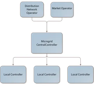
Market Operator

Microgrid CentralController

Local Controller Local Controller Local Controller Distribution

Network Operator

There are two-levels to microgrid control: a microgrid central controller (often referred to as microgrid controller), and local controllers. The microgrid controller is required to run long-term and real-time optimal dispatch, thereby providing optimal set-points for the supply of electrical and thermal energy. The control should also supervise the microgrid to maintain voltage and frequency stability, ensuring power quality. The controller also needs to be making the right decisions when a failure occurs, or manage black start subsequent to a failure. The microgrid controller needs also to ensure the participation in the energy market, and provisioning the microgrid for ancillary service.

Each microgrid asset or a combination of them contains one local controller to apply commands from the central controller and control their own parameters at desired level. Depending on the control approach, each local controller may have a certain level of

intelligence. In a centralized control strategy, each local controller receives commands from the corresponding microgrid controller (central controller) for some of the operating

parameters. In a decentralized control strategy, each local controller makes decisions locally on more parameters, leaving less space for the central controller to participate. Also some decisions can only be made locally in either approach, like a local controller does not need a command for voltage control. [7]

normally are not counted as parts of the microgrid; they are more like delegates of the whole electric grid which effect microgrid through decisions made by microgrid controller. So in this thesis we would not lay much importance on them.

1.1.3 Microgrid Modeling

In the process of microgrid controller developing and commissioning, it’s not very possible

to connect the controller with a real microgrid and operate. In order to test the functionalities of a microgrid controller, a microgrid testbed is needed. Planning and operating microgrid decisions directly depend on modeling of the microgrid, and test results of microgrid controller operating on the microgrid model. To make sure the microgrid controller is capable of making reasonable technical and commercial decisions, the models should reflect the real world accurately and clearly.

CHP Energy Storage Substation Feeds Transformer CB CB CB Feeder A Feeder B

Main Grid Microgrid

CB

CB Transformer

Figure 1. 4 An example microgrid one-line diagram [20]

1.2 Microgrid Examples

Microgrid projects have been undergoing a fast increase for the last few years. The following contents will present several microgrid examples of projects, accomplished or still under construction, which provided their value in critical situations.

1.2.1 New York University

As one of the largest universities in the United States, New York University has been producing power on site since the 1960s and installed a large oil-fired cogeneration plant in 1980. At the end of that facility’s service life, NYU made a decision to transit from oil-fired

The CHP system has an output capacity of 13.4 MW (twice as much as the old plant’s capacity) and has been fully operational since 2011, supplying power to 22 buildings and heat to 37 buildings. The microgrid consists of two 5.5 MW gas turbines for producing electricity coupled with heat recovery steam generators and a 2.4 MW steam turbine. The NYU microgrid is connected to wider area distribution grid and purchases electricity when demand cannot be met on site.

Based on microgrid upgrades, the NYU microgrid is now able to operate in island-mode and disconnect from grid. It has been successfully tested during Hurricane Sandy, when the NYU microgrid successfully islanded from the local distribution grid and continued to reliably power much of the NYU campus.

The transition towards microgrid implementation of the plant has proven its benefits both economically and environmentally. Savings on total energy costs is $5 to $8 million per year, evaluated by NYU. It also reduced NYU’s local emissions drastically, with an estimated 68% decrease in EPA criteria pollutants (NOx, SO2, and CO emissions) and 23% decrease in

greenhouse gas emissions. This is a great step towards the commitment the university made to the City of New York—to decrease its greenhouse gas emissions by 30%.

1.2.2 Borrego Spring Microgrid

innovative microgrid that integrates the distributed resources and resources on the customer‐

side. [10] The goal of the project is to provide a proof-of-concept test as how microgrid—or information technologies and distributed energy resources combined together can increase utility asset utilization and reliability.

Figure 1. 5 Borrego Spring Microgrid Architecture [21]

The total capacity of the microgrid will be about 4 MW, including two 1.8 MW diesel generators, a large 500 kW/1500 kWh battery at the substation, three smaller 50 kWh

batteries, six 4 kW/8 kWh home energy storage units, about 700 kW of rooftop solar PV, and 125 residential home area network systems. [11] The community is an isolated area fed only by a single sub-transmission line. Now islanding of the entire microgrid is being

demonstrated for reliability verification. By using the smart meters and home area network devices, SDG&E is also exploring the price driven demand response possibilities, via interacting with storage devices, electric vehicles, and smart appliances. Supervisory control and data acquisition (SCADA) is incorporated on all circuit breakers and capacitor banks, Feeder Automation System Technologies (FAST), outage management systems, and price driven load management at the customer level.

1.2.3 Sendai Microgrid

The Sendai Microgrid Project, one of the most well-known microgrid demonstrations, was one of the four major New Energy and Industrial Technology Development Organization (NEDO) projects carried out in Japan. It is located on the campus of Tohoku Fukushi University in Sendai City in the Tohoku district, and initially was designed in 2004 as a test bed for a demonstration project of the NEDO. The study was completed in 2008, and after that the microgrid system continued to operate as a highly successful project.

extreme devastation, the Sendai Microgrid continued to supply power and heat to customers, proving its effectiveness and excellent performance, thus becoming a microgrid

superstardom known world widely. [12] After a few hours of service loss, generators on site were started and the microgrid supplied the teaching hospital of Tohuku Fukushi University with both power and heat during the two-day blackout.

1.3 Project Background

The work described in this thesis is part of the Department of Energy Olney Town Center Microgrid project. This project will design and develop a microgrid controller, namely Green Energy Bus, to provide Montgomery County, Md. with developed and lab-tested control system technology options, to increase the resiliency of the Olney Town Center area.

The Montgomery County Planning Board in 2005 established the Olney Town Center as “a civic center/town commons”, not only because it serves as a key point of interaction in the

Figure 1. 7 Olney Town nodes map

These features make the Olney Town Center an ideal candidate when considering microgrid deployment. If this center of essential services is operating properly with microgrid deployed, the Olney community could function normally for weeks even during a regional outage. To allow the community to achieve greater resilience, obviously a more powerful, extensible, and cost-effective microgrid control system is needed.

To achieve the community’s objectives, the Olney Town Microgrid team will design a

the system will reduce the Town Center’s carbon footprint by 20%, and improve its energy efficiency by at least 20%.

The role of FREEDM Center in this project is to lead and execute all microgrid control systems testing for the project, and supports engineering analysis and test results reporting. In other words, FREEDM Center is in charge of designing and developing a microgrid

simulation model to test the effectiveness of the microgrid controller developed by Green Energy Corp. And my task in this project is mainly to build DNP3 communication interface in model, and launch model validation tests as well as communication tests.

1.4 Content of Thesis

In this thesis, how a microgrid model is designed and built, how to validate effectiveness the model, and how the communication interfaces between model and a test-oriented “controller” are established is discussed.

Chapter II. Olney Microgrid Components

2.1 Olney Town Microgrid Project Overview

As mentioned in the first chapter, the Olney Town Center Microgrid project will be focusing on researching, developing, and testing microgrid control systems FOR Olney Town Center. To provide an enhanced understanding of factors affecting community microgrid control system design requires a simulation for Olney microgrid and its operating conditions in various scenarios.

Thus a well-designed model of the Olney Town distribution grid is a primary need. Information of the grid assets and their capacities, connection of these components, and different scenarios for PV and grid connection is of vital importance when building and emulating the microgrid. Also, the control goal of the controller’s economic and

environmental objectives should be clarified before design and development of the

simulation. To introduce the expected functions, goals targeted should be made clear. The objectives of the microgrid controller are simply the Department of Energy (DOE) goals: a) Reducing outage time of critical loads by more than 98%; b) Reducing emissions by 20%; and c) Improving system efficiencies by more than 20%.

System Average Interruption Duration Index (SAIDI). Satisfactory accomplishment of reducing emission would be demonstrated by testing that indicating 20% reduction in emissions be achieved attributable to operation of the proposed microgrid. And a test demonstrating that the total utility-supplied electrical and thermal is at least 20% less after deployment of the proposed microgrid than that before, can be a sufficient principle which proves the efficiency goal met.

Functions for the microgrid controller including: disconnection; resynchronization and reconnection to the grid; steady-state frequency and voltage control; energy dispatch; black start; and ancillary services. The Olney Town project provides multiple user cases for various functionalities, indicating brief action sequences about how the controller and components would react in specific environments. In this thesis these use cases with controller behavior focus are used to develop testing plans for model validation. Though it’s not practical to build all models and test them in all scenarios, most of the test plans are listed and several of them are conducted and results are shown. What will be considered first is whether the model can support the static energy dispatch function of the microgrid controller.

2.2 Microgrid Components

system, absorption chiller and loads will be included. The community is connected to utility through utility Point of Common Coupling (PCC). The total electric load will be around 7 MW.

In order to initiate a basic testbed, FREED Center developed a generic microgrid model referred to as “Zone 0” for component modeling. The grid components for the Zone 0 model

are shown below in figure 2.1:

Substation Substation Bus ZONE 0 FREEDM Test System ESS High Priority Load PV ABS Medium Priority Load Optional Priority Load DC AC AC DC Absorption Chiller PCC PCC NG CHP

This system contains each of the different components of Olney Town microgrid. Loads are actually integrated together as one load using all different levels of loads. The absorption chiller is connected to the Combined Heat and Power (CHP) unit. At this time CHP unit model focuses on its static performance, and by now doesn’t include any dynamic modeling.

2.3 Olney Town Microgrid Modeling

The first thing should be considered when developing the real-time microgrid model is the simulation platform.

Real-time simulation is used in many engineering fields and applications. These applications benefit from the use of real-time simulators in the following ways. First, it enables testing of simulated devices at or beyond their normal operating limits, without risking damage with real devices, especially when high power levels are involved. Second, the simulation acceleration factor obtained by the use of compiled code enables the realization of rapid batch simulations [8].

converted to analog outputs, which are in turn sent to the hardware system to accomplish a typical HIL test circle [9].

To benefit from a Hardware-in-the-Loop testing on a real-time simulator, in this project RT-LAB from OPAL-RT Technologies Inc. is chosen as simulation platform. It is real-time simulation software which is fully integrated with Matlab/Simulink. The plan of simulation is to develop and run separate components models in Simulink first, then integrate them and run in RT-LAB with designed scenarios.

2.3.1 Combined Heat and Power

Cogeneration or Combined Heat and Power (CHP) is the use of a heat engine or power station to simultaneously generate electricity and useful heat. At smaller scales (typically below 1 MW) a gas engine or diesel engine may be used. Cogeneration is a

thermodynamically efficient use of fuel. In separate production of electricity, some energy must be discarded as waste heat, but in cogeneration this thermal energy is put to use. All thermal power plants emit heat during electricity generation, which can be released into the natural environment through cooling towers, flue gas, or by other means. In contrast,

CHP captures some or all of the by-product for heating, either very close to the plant, or as hot water for district heating with temperatures ranging from approximately 80 to 130 ℃.

unit is turbine-generation based, generate electricity and utilize waste heat to increase efficiency.

Figure 2. 2 CHP unit energy flow

In the Olney Town project, CHP is modeled together with absorption chiller. A load model is also added, but as a mathematical model to calculate energy, rather than the load models we connect to the main bus as microgrid components.

Heat Recovery unit

Gas Turbine Generator

Water

Hot Water or Steam

Heating or Cooling

Building or Facility

Power Grid

Fuel

Figure 2. 3 CHP and absorption chiller model The table below shows all inputs and outputs of the model.

Table 2. 1 CHP inputs and outputs

Model inputs Model outputs

P_ref: output real power target. a, b, c: Three phase electricity wavesforms which represent electricity the CHP unit injects into the main bus.

Enable: CHP turbine enable signal. Parameters of the model which can be measured, like turbine waste temperature, energy in BTU/h, real and reactive power in watts.

2.3.2 Photovoltaic System

A photovoltaic power system is a power system designed to supply usable solar power by means of conversion of solar energy to electric power. It consists of an arrangement of several components, including solar panels to absorb and directly convert sunlight into electricity, a solar inverter to change the electrical current from DC to AC, as well as mounting, cabling and other electrical accessories to set-up a working system.

The PV modeling in the project is currently using real 5-minute measurement solar data to create a solar radiation database. To fulfill the microgrid controller data resolution

requirements, the 5-minutes data is resampled to higher resolution using interpolation. The real solar data contain 3 day types: Sunny, Partial Cloudy, Cloudy, allowing selecting solar profiles randomly. Storms and clouds effects can also be added at designated time intervals. Similar to the other components, it is connected to an inverter before connecting to the main bus.

Figure 2.3 shows the PV model in Simulink, and figure below shows the other part of PV model in OPAL. Existing PV solar data is stored in a file, read into the system by blocks “OPFromFile” in OPAL and fed into the model through user defined input “P_ref”. Since the

PV model is designed to use pre-defined data, a method is needed to convert these RMS values into real time sinusoidal waves which represent electricity flows in the grid. Figure 2.4 shows how this is achieved. Note this involves converting 1 minute interval RMS values into three phase sinusoidal waves with 120 degree phase difference and same amplitude.

Table 2. 2 Photovoltaic model inputs and outputs Model inputs Model outputs

P_ref: Solar data. Three phase electricity flow which fed into the main bus.

Enable: enable signal of the model. Parameters of the model which can be measured, like voltage, current, real and reactive power.

2.3.3 Energy Storage

Energy storage is accomplished by devices or physical media that store energy to perform useful processes at a later time. A device that stores energy is sometimes called an

accumulator. Many forms of energy produce useful work, heating or cooling to meet societal needs. These energy forms include chemical energy, gravitational potential energy, electrical potential, electricity, temperature differences, latent heat, and kinetic energy. Energy storage involves converting energy from forms that are difficult to store (electricity, kinetic energy, etc.) to more conveniently or economically storable forms.

Figure 2. 6 Battery block equivalent circuit in Matlab

Energy storage model inputs and outputs are listed in Table 2.3.

Table 2. 3 Energy Storage Unit model inputs and outputs

Model inputs Model outputs

V_PCC : Main bus voltage Three phase electricity feed into main bus. P_ref: Output real power reference SOC: State of charge of the battery.

2.3.4 Customer Electric Load Model

resolution, additional 15-minute residential load data based on PNNL field demos are introduced to the model. Similar to the PV model, the hourly data is resampled to get higher resolution using interpolation. The load model is setup for both summer and winter day types, with four load priorities: High, Medium, Low, and Optional. The model allows a random selection of load profiles, which includes modeling of cycling loads such as air conditioning

Figure 2. 7 Static load model

The implementation of the load model in this project is similar to the PV model. Pre-defined RMS data is converted it into real time three phase sinusoidal waves and connected with the main bus. Below the figure 2.8 shows how RT-LAB supports us with file reading

Figure 2. 8 Read file scheme in RT-LAB

Table 2. 4 Load model inputs and outputs Model inputs Model outputs

Chapter III. DNP3 Protocol and Communication Interface

3.1 DNP3 Overview

DNP3 (Distributed Network Protocol, version 3) is a telecommunication standard that

defines communications between master stations and outstations.[5] It was developed by GE, previously Harris, Westronics, and it was based on the early parts of the IEC 60870-5

Reasons why DNP3 is so widely used is based on the benefits it brings to utilities. As an open standard, DNP3 provides interoperability between equipment from different manufacturers. Users can purchase master stations from one manufacturer and RTU equipment from another manufacturer. Other benefits include:

 Supported by an active DNP3 User Group;

 Widely adopted by large and increasing group of manufacturers;  It has a layered architecture conforming to IEC enhanced performance

architecture model;

 Optimized for reliable and efficient SCADA communications.

DNP3 utilizes three layers of the OSI 7-layers model, called Enhanced Performance Architecture. The three layers are the application layer, transport layer and data link layer. Each layer contains a header which would either help transport the message or indicate functionalities. Data is categorized as class 0, 1, 2 and 3 in DNP3 protocol. Static data, meaning current value of a point, is assigned to class 0. Event data, meaning something significant happens can be assigned to class 1, 2 or 3. Data in class 1, 2 and 3 is also in class 0, meaning that polls for class 0 data actually polls for all classes. The DNP3 protocol does not assign any significance between class 1 2 and 3, they can be defined by users.

outstation send data changes or events without master station polling, and it’s often used

when the master station needs to reply on outstation to send specific event data actively.

3.2 Implementation for Project Application

Communication interface in this project contains two parts: DNP3 master station and DNP3 outstation (DNP3 slave). DNP3 outstation interface is integrated into the microgrid model. It responses to master station poll, receives outputs from master station and delivers them to microgrid model. The microgrid controller designed by Green Energy Corporation (namely Green Bus) serves as DNP3 master station in communication infrastructure. Tests referred to in this thesis use another master station developed in LabVIEW platform, and the other protocol test software Protocol Test Harness.

Microgrid controller Green Bus

Microgrid testbed Master station in

LabVIEW Protocol Test Harness

In project

For test purpose

For test purpose

Data transfer between master station and outstation are mainly analog inputs, analog outputs, binary inputs and binary outputs. Analog inputs are signed numeric values, either physical values—like voltage or frequency of the model, or calculated values—like efficiency.

Analog outputs are also signed numeric values, but they originate from the master station and often function as setpoints of a desired operating level .Binary inputs are single-bit Boolean type values, usually standing for on or off status. Binary outputs are commonly referred to as Control Relay Output Block (CROB), and in this project we’ll use it to control switch and relay to open or close. Unsolicited message is also enabled, to make sure the outstation has the capability to send an alarm signal whenever a value exceeds its pre-defined threshold.

3.3 Communication System Setup

Figure 3. 3 DNP3 communication infrastructure (with relay in loop)

3.4 Master Interface in LabVIEW

A DNP3 master station is designed and developed in LabVIEW to increase the flexibility in system testing. As a graphical automation system design tool, LabVIEW can provide more flexibility in conducting the test and validation process.

The DNP3 master interface is based on DNP3 tool box in LabVIEW. The Virtual

Instruments (often referred to as VI in LabVIEW, it’s the basic building block of programs written in LabVIEW. It is similar to a function or subroutine in other programming languages) implement DNP3 protocol stacks to achieve its communication functionalities. Master

station programming contains various VIs in this tool box to achieve different control commands over DNP3 slave station. The execution flowchart is shown in figure below.

Microgrid Controller

SEL 451

Communication Connection: DNP3

Microgrid Model

Start

Check pre-entered network parameters

Connection built?

Polling start

Polling failed, return timeout

Send command?

Return success

Return timeout Yes

No

Success

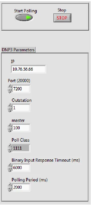
The programming environment in LabVIEW contains two parts: front panel and block diagram. The front panel is often used as Human Machine Interface in LabVIEW

programming, and the block diagram is the programming underneath interface. The front panel is also divided into two parts, DNP3 parameters and microgrid components data. These are shown separately in figure 3.5 and 3.6.

Figure 3. 6 Microgrid components interface

interface development is shown in thesis work, and Energy Storage unit tab is chosen to illustrate basic control capabilities of DNP3 master interface in LabVIEW.

The block diagram contains the graphical source code of a LabVIEW program. The concept of the block diagram is to separate the graphical source code from the user interface in a logical and simple manner. Terminals on the block diagram reflect the changes made to their corresponding front panel, often considered as terminals of the block diagram, and vice versa. The block diagram programming will be listed in Appendix C.

Analog inputs and binary inputs are shown in the top-left corner in Figure 3.6. Binary inputs are referred to by indexes and indicated by light indicators. Analog inputs are located by indexes and shown by numeric values, and charts are also used to show the trending and part history data of analog inputs. Setpoint control is analog output control in DNP3, which sends out analog values as setpoints to the slave station. Relay control, or CROB (Control Relay Output Block), is binary output in DNP3. It’s used to control breakers and other parameters

which only have two statuses.

Detailed communication tests and results will be shown in Chapter VI.

3.5 Slave Interface in OPAL-RT

for the model are one part of it, called DNP3 slave interface. It consists of one asynchronized DNP3 block, and all analog and binary points.

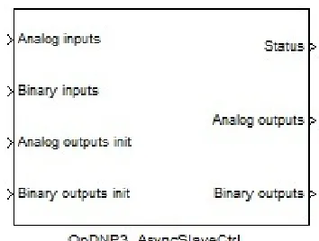
3.5.1 RT-LAB DNP3 Block

RT-LAB has one block designed for simple DNP3 communication as a slave station, and it’s shown below.

Figure 3. 7 DNP3 block in RT-LAB

b) It is not used by other devices.

The value “Configuration file name” in property block should correspond to the real XML file name located in the project folder.

3.5.2 Points List

When setting the block, one thing of great importance is the number of inputs. Drawing model outputs and feeding them into the block should also be done manually because the block does not get the values automatically. To appropriately prepare the model with matching interface, we need to know what points are designed to feed the microgrid

controller and thus build the corresponding points into the model. Points are divided into four categories: analog input (AI), analog output (AO), binary input (BI) and binary output (BO). Outputs are control commands like trip/close, set points. Inputs are measured physical values, predefined ratings or status. No counters are involved in the project at this phase.

Table 3. 1 DNP3 Points of Point of Common Coupling*

Added? Name Type Unit Comment

Y kW Analog Input kW This is the measured power come from whole grid. Positive value stands for power

consumed by microgrid, and negative power means power flow from microgrid to whole grid.

Y kV Analog Input kV Voltage at Point of Common Coupling.

Y Amps Analog Input A Current at Point of Common Coupling.

N PwrFact Analog Input Power factor of power.

N Hz Analog Input Hz Frequency at Point of Common Coupling.

N Status Binary Input Status of this Point of Common Coupling, open or closed. N Trip Binary Output Trip the breaker.

N Close Binary Output Close the breaker.

* PCC_Head and PCC_Tail have the same point list.

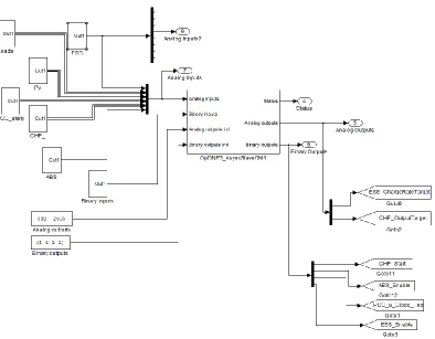
3.5.3 Slave Device Interface

to show the user real time data. The feature of showing real time data is crucial to

communication testing, thus the DNP3 interface in model is assigned to both subsystems. Communication testing is the first step before executing any other tests, to ensure the model has sufficient communicating capability. This test should include two parts, substantiating the interface is capable of supporting DNP3 in two directions—both receiving and

transmitting data. This testing will be further discussed in Chapter 6.

Chapter IV. Microgrid Controller Use Cases and Simulation Validation

After introducing models for different components and communication part in the microgrid simulation system, it’s necessary to further understand and discuss the design behind them

from controller stand of point. Also, simulation validation is needed to convince the built of models meet our original designing goal.

4.1 Microgrid Controller Functionalities

The microgrid controller is designed to maintain voltage and frequency to a pre-defined level, as well as managing energy and securing microgrid islanding operation mode. For the energy management function, the central controller optimizes the power microgrid exchanges with the whole electric grid, maximizing the local production from distributed energy resources depending on the market prices and security constraints. It is achieved by issuing control set points to distributed energy units and controllable loads within the microgrid. The

communication can be through Ethernet, power line carrier, or wireless network. Normally the controller makes decisions for a specified time intervals such as every 15 minutes for the next hours or a day. [7]

the community within the territory by initiating a blackstart. Voltage and frequency control are two key problems during a blackstart. After the microgrid is operating successfully in an island mode and the whole grid gets back to normal, the microgrid may need to reconnect to it. This is where the problem of transition from island to grid-connected introduced. A microgrid central controller needs corresponding strategies to deal with all problems above.

Microgrid Central Controller

Functional Requirements

Non-Functional Requirements

F1 Frequency Control

F2 Voltage Control

F3 Intentional Islanding

F4 Unintentional Islanding

F5 Islanding to Grid Connected Transition

F6 Energy Management

F7 Microgrid Protection

F8 Ancillary Services

F9 Microgrid Blackstart

F10 User Inerface and Data Management

Trustworthiness

Configuration Management

Scalability

Interoperability

Figure 4.1 illustrates requirements that drive microgrid controller functionalities. These requirements are divided into two categories: Functional and Non-functional. Functional requirements are described briefly in the above paragraph, and they are considered and designed to achieve the control capability over a microgrid. Non-functional requirements are based on the consideration that it’s at the same time software which should be easily

managed, maintained and implemented into the whole control system without causing any security problems.

4.2 Use Cases

Electric Power Research Institute (EPRI) proposed several microgrid functional user cases as a guide that shows how the controller should accomplish these important functionalities. These use cases are adopted by Green Energy Corp in microgrid controller design.

These use cases include: Frequency Control, Voltage Control, Intentional Islanding, Unintentional Islanding, Island to Grid Connected Transition, Energy Management, Microgrid Protection, Ancillary Services, Microgrid Blackstart, User Interface and Data Management. The use case this project is most concerned about is the Energy Management user case. Through validating the controller’s capability on this user case, this project can meet the energy efficiency enhancement requirement proposed by DOE.

4.2.1 Energy Management

and the microgrid. The microgrid EMS manages the power flow, power transaction, energy generation and consumption, voltage/reactive power, and battery charging/discharging in a microgrid. The objective of the Microgrid EMS is to coordinate among multiple DERs, storage/battery, main grid and responsive loads to improve the system reliability and reduce the total operation cost.

The optimization objectives are achieved by deploying a three-stage energy management: Day ahead Bidding and Scheduling, Short-term Economic Dispatch and Real-time Optimal Power Flow (OPF).

The Day-ahead Bidding and Scheduling stage includes the function of day-ahead operation planning. The plan is developed on the day before the actual operation, and can be updated on the day of operation. It contains the optimal bidding and scheduling plan for electricity and heat (at hourly interval) for the next day, based on the demand forecast, renewable DER output and market prices. Normally, in developing this plan, the unit commitment status and output dispatch of DERs and the power purchased/sold in the day-ahead market are

4.3.2 Microgrid Blackstart

After a complete shutdown, blackstart is executed to restore the microgrid which is in island operation mode. The process involves the microgrid central controller, distributed resources, loads, and multiple circuit breakers. The blackstart procedure can be pre-determined and implemented in the microgrid central controller and other devices based on the system topology, sizes of resources and loads. There a few main steps involved in the execution of the microgrid blackstart.

4.3 Simulation Validation Methodology

Figuring out a fundamental methodology of simulation validation is especially important where the credibility of a simulation model is crucial. In such cases decisions need to be made in complex situation, or where simulations can provide incentives for decision maker either due to lack of access to the real system or as a sort of prior assessment. In other situations, it is important to understand the potential risks involved when using a simulation: A simulation model may not adequately represent the real world system; the data used may be inaccurate; or it may not be practical to model the exact operational environment. Even the output data gathered to build the model may be flawed in some way or somehow misinterpreted. [16] Either way, a certain quality assurance of the model is needed, and simulation validation, as a way of checking and providing this assurance, is brought out and studied. [15] It will also support decisions on basic concepts, system design, and feasibility of operation without the expense of developing prototypes or test models.

To introduce basics of simulation validation, we need to consider several basic features of simulation. Simulation is the process of a) constructing a model of a system, and b)

Simulation studies of power systems can be dated back in 1960s, but the importance of its validation and assessment was not noticed until the model actually failed and caused huge loss—known as the WSCC system outage on August 10, 1996, where the failure of simulation in reproducing the dynamic behaviors prior to real system implementation was considered to be one main cause. [14]

In the Olney project, microgrid model simulation is conducted to accomplish the goal of controller testing and demonstration. And since we understand importance of simulation validation, we want to show our model is capable of supporting the tests in developing simulation validation.

Due to differences in simulation fields, aiming application, and various simulation methods, we do not yet have a quantitative measure of the level of validation performed on a

simulation model. However, there are some principles to consider when conducting simulation validation type of research.

First, the simulation validation and verification study (will be referred to as simulation validation in following content) should be conducted throughout the entire life cycle of the study. It’s not a step which we can ignore once we complete it, but a continuing process to correct errors and enhance the model. Second, a simulation model is built with respect to the study objectives, so its credibility should only be judged with respect to those objectives. And similarly, credibility of a simulation model can only be claimed in the prescribed conditions in which the model is built and tested. And normally this study of simulation validation is conducted by different researchers other than the model developer, in order to prevent any intentional or unintentional bias. And last but not least, credibility given by each submodel does not guarantee overall model credibility. [13] They should be tested separately.

Chapter V. Microgrid Model Tests

5.1 Single Model Test Plans

The first thing to do in model validation is to make sure every single model works fine. Thus we need to fully understand how the model works, then test if it performs as designed and expected.

One important feature of each model that needs to be tested is the energy output. Test results are shown in the following sections to justify models capability to generate reasonable output. One assumption made to examine the power flow is that, for a given unit, minus power

output means it’s absorbing power, and positive output means it’s providing the main bus

with power, either real or reactive.

5.1.1 Load Output Verification

Figure 5. 1 Load group test setup

Figure 5.2 shows the 24-hour load profile used in this test. At the time the scope screenshot was taken, the real power value should be equal to the value found in this profile at the same time.

From the result shown in Figure 5.3, we can see the real power is 32.84kW at time 6.05s, which is very close to the valure found in the load profile at about the same time. Also the product of voltage and current is 11911.62W, which is very close to one third (load is

5.1.2 Photovoltaic Model

Similarly, PV model validation is done by checking power output read in the scope, and comparing the value with the solar profile at the same time.

The start point of the test is chosen to be index 500 since there’s not much output power

before this index. The screenshot of PV output shows PV power output in kW and the percent of output to capacity. At time 3.6s, a time stamp relative to the start point chosen when conducting this test, the output is 122.6kW. It’s found out that similar value in the figure at the same time (around index 503.6) in solar profile. Thus the model operates normally.

5.1.3 Energy Storage Unit Model

Testing the energy storage unit is performed by comparing the power output and charge/ discharge rate with the predefined output target. A constant 25 kW is given as the output target for the ESS unit to achieve. From the second subplot in the screenshot of scope, we can see that the actual output rate is very close to this target. So the ESS unit model meets our expectation for testing by far.

Figure 5. 8 ESS outputs of SOC and Charge/Discharge Rate

5.1.4 Combined Heat and Power and Absorption Chiller

For the CHP model, the actual output power is measured and compared with the output target, 250kW in this case. A screenshot of the output shows a result of 249.96 kW, which is close enough to say the CHP output can be controller as expected.

Figure 5. 9 CHP model setup

Another output for the CHP unit to examine is the waste heat temperature. A pre-defined limit is 185 degree Centigrade, which is 365 degree Fahrenheit. The screenshot below shows the real waste temperature, which falls within the limitation of 365.

Figure 5. 11 CHP waste heat temperatures 5.2 FREEDM Zone 1 Microgrid Power Flow Test

The test is done in FREEDM test system zone 1. Unlike zone 0, zone 1 contains more units, including 10 loads and 3 PV units, one unit for CHP, ABS and ESS. Power flow should be measured and checked for aggregated groups, which means all loads are monitored as one load group, and PVs are measured in this way also.

Substation Substation Bus ZONE 1 FREEDM Test System ESS Rooftop PV System 1

ABS _{Rooftop PV System 2 Solar Tree}

PCC_cbr_cust PCC_cbr_util DC AC AC DC AC DC AC DC Absorption Chiller NG-CHP Load Group 1-10

Figure 5. 12 FREEDM Test System Zone 1

By running the system and displaying all real and reactive power provided by all components, fed by whole grid at PCC and line loss between main bus and all components, we can

Table 6. 1 Power flow result 1

Real power (kW) Reactive power (kVAR)

PV 0 0

ESS 25 0.4712

CHP 189.1 3.565

Load -33.14 -14.19

Line loss* -1.883 × 10−4 ₀

Sum of microgrid generation 180.96 -10.06

Power injected to microgrid -181 10.15

* Line loss is calculated by equation 3(I2× Z), where I = 7.923 A and Z = 0.001Ω, and minus stands for power consuming.

Table 6. 2 Power flow result 2

Real power (kW) Reactive power (kVAR)

PV 121.2 2.284

ESS 25 0.4712

CHP 80.65 1.52

Load -32.65 -13.97

Line loss* -2.164 × 10−4 ₀

Sum of microgrid generation 194.2 -9.695

Power injected to microgrid -194.2 9.699

Chapter VI. Communication Tests and Results

Communication capability is one important feature the model needs to provide, and is not examined in previous model tests. As planned in the project, DNP3 protocol needs to be implemented and tested. This chapter mainly focuses on communication test, in other words, DNP3 communication tests design and examination.

Two DNP3 master stations are used in the test. Protocol Test Harness is used to test DNP3 functionalities of microgrid testbed. After the testbed is checked for slave station capability, the LabVIEW master station is tested using testbed to prove its DNP3 master station

capability.

The reason to arrange tests for LabVIEW is that it can provide more flexibility in exercising future tests. Potential benefits include test automation and history recording. For example in energy dispatch test, the OPAL simulator may need to run for a whole day. In this case it’s

not possible to manually send all dispatch commands in pre-defined time schedule. So an automated commands sending scheme is crucial. On the other hand, OPAL has a limited storage capacity, leaving the role of data recording to master station. LabVIEW master station is on another computer which has enough storage. The LabVIEW platform is also more flexible in data logging format.

Protocol Test Harness [6], developed by Triangle Microworks, is a powerful tool for testing DNP3, IEC 60870-5, and Modbus devices. It can simulate master or outstation devices in different communication protocols, and run in monitor mode. Test Harness is also capable of creating custom functional tests with any .NET programming language, and performing conformance test procedures as well.

In this project, this tool is used to simulate a DNP3 master to test the communication capability of the model, so a connection between Test harness as DNP master station and microgrid model as DNP outstation in RT-LAB is built. On configuring the outstation with proper IP address, port number and link layer addresses (which was discussed in Chapter 4), the microgrid testbed is prepared by loading the configuration files. Then the corresponding parameters of DNP channel and session are input into Test Harness to build a new

workspace. Figure 6.1 shows the main interface when the DNP3 connection is established between master and outstation.

Test Harness is capable of sending commands as well as polling data based on class via its command window. The DNP command window can also enable/ disable unsolicited messages and send time synchronization signal. These functions are checked in the tests, since the DNP slave control block in RT-LAB claims to support all of them.

6.2 Communication Tests and Results

To make sure the model responds to analog outputs, both the data received and

corresponding response need to be checked. As is shown in Figure 6.2, analog output initial values are received in Test Harness. The verification is done by sending analog outputs using Command Window and checking results in the model.

Figure 6. 2 Analog output initials received in Test Harness

The analog output point chosen to test is “ESS_ChargeRate Target”. This is the output target

of the energy storage unit, and analog input point “ESS_ChgDischgRate” is the real output of energy storage unit, which in all cases should be consistent with “ESS_ChargeRate Target”.

First change the value of “ESS_ChargeRate Target” from the command window, then checking this value received in outstation. Secondly the real output is checked to see if the model is capable of supporting analog output.

The analog output of the charge rate target, with value of 3500 kW is sent through the command window with result shown in Figure 6.5. Though a small error exists, the outstation function to response to analog output is validated.

Figure 6. 5 ESS_ChargeRate Target and ESS_ChgDischgRate values A similar method is used when testing the model’s binary outputs response.

All three binary outputs should be 1 instead of 0 in Test Harness. This observation turns out to be a bug of “OpDNP3_AsyncSlaveCtrl” block in RT-LAB version 10.5, which is

corrected in version 11.0, claimed by their technical support team. Yet by the time this test is conducted, RT-LAB 11.0 is not installed in the test platform. So the bug of initial values of binary output is recorded, and the ability of receiving binary output and executing the command is tested in this thesis.

Figure 6. 7 DNP3 points configuration in outstation

The binary output point “CHP_Start” is chosen in order to examine the binary output

Figure 6. 8 Command window of binary output

Figure 6. 9 CHP_Start and CHP_kW_tot value change

Figure 6. 10 Poll for analog inputs

Figure 6. 11 Poll for binary inputs

6.2.2 Time Synchronization

Time synchronization capability is supported by the DNP3 interface in the microgrid model. By sending time synchronization commands through command window in Test Harness, we can see the binary inputs sent back with time stamps.

Figure 6. 12 Time Synchronization command window

Figure 6. 13 Binary Input Change with time stamp

Whether the data contains a time stamp or not is also subject to DNP3 object variation. Object 2, variation 3, also referred to as Binary Input Change with time stamp, is generated and reported when there’s a change of binary input points. Yet Object 32, variation 1, which

refers to Analog Change Event without time stamp, does not contain any time stamps. These variation types are pre-defined in DNP3 functionalities in RT-LAB. So after time is

6.2.3 Enable Unsolicited Message

Data exchange functionalities including response to polling, receiving outputs and executing commands are tested and validated in this chapter. The abilities to support time

synchronization and unsolicited message are also examined. Thus the conclusion that the microgrid model in RT-LAB supports basic DNP3 communication capabilities can be drawn.

6.3 LabVIEW DNP3 Interface Test

The prototype DNP3 master station interface described in Chapter III is tested here to make sure it has basic data exchange capability. The test examined four data types: analog input, binary input, analog output (setpoint) and binary output (control). The component used in this test is the Energy Storage Unit (ESS). An extra control point “ESS_Enable” is added for test purpose.

The analog point with index 0 is the ESS capacity, which is a constant with value 129 (kW). The analog point with index 3 is ESS real power output, “ESS_ChgDischgRate”, which should follow the value of setpoint “ESS_ChargeRate Target”. The point

“ESS_ChgDischgRate” also indicates if the unit is enabled or not. The binary output point “ESS_Enable” has an index of 3 and default value of 0, which means the Energy Storage

Figure 6. 16 Energy Storage Unit enabled

Figure 6.16 above shows the analog input with index 3 has experienced a change from 0 to 40 in enabling the unit. Thus the binary output works in DNP3 communication. Then the second step is to examine setpoint “ESS_ChargeRate Target” with index 0. The original

Figure 6. 17 Setpoint change in ESS unit

By changing the binary input index, the capability of correctly receiving binary inputs is examined. The binary input with index 3 is 1 (or ON) and the other binary input with index 4 is 0 (or OFF). These values are the same with the system setting, thus the binary input data type is also supported by LabVIEW.

Figure 6. 18 Binary inputs values in LabVIEW

Chapter VII. Conclusions and Future Work

The thesis work focuses on implementing DNP3 protocol into a microgrid testbed and testbed validation. The first 2 chapters provide background information about microgrids, and the Olney Town Microgrid project which the thesis is part of. The third chapter

introduces DNP3 protocol and a method of implementing it into the testbed. Chapter Four explains what simulation validation is and why it is needed. Several test plans are given for future reference. Chapter Five and Six focus on tests and their results, including single model tests and communication tests.

The Olney Town Microgrid project is still a work in process. Though a lot of effort was put into supporting the communication and validation parts in doing the thesis, there is still a lot work to be done.

A DNP3 master interface based on LabVIEW platform is introduced in Chapter Three and tested in Chapter Six, though there’s still opportunity to further enhance its performance. Functionalities like file reading and automated commands sending should be explored when automating test process using LabVIEW. Theoretically this platform is also capable of recording data, further processing data and creating a more user-friendly Human Machine Interface. These are options should be considered in future development within.

hardware system is being building up and not much detail is available. So the test plans aiming to further explore model capability in supporting microgrid controller use cases need to be considered and enhanced before commissioning.

REFERENCES

[1] Schwaegerl, Christine, and Liang Tao. "The Microgrids Concept." Microgrids: Architectures and Control (ed N. Hatziargyriou), John Wiley and Sons Ltd, Chichester,

United Kingdom. doi 10 (2013): 9781118720677.

[2] Zadeh, M. R. D., et al. "Design and implementation of a microgrid controller."Protective Relay Engineers, 2011 64th Annual Conference for. IEEE, 2011.

[3] Kosterev D, Meklin A. Load Modeling in WECC[C]. IEEE Power System Conference And Exposition, 2006.

[4] www.energy.gov

[5] “The World Market for Substation Automation and Integration Programs in Electric Utilities: 2005-2007,” Newton-Evans Research, September 2005.

[6] http://www.trianglemicroworks.com/

[7] Ktiraei, F., et al. "Microgrids management-controls and operation aspects of microgrids." IEEE Power Energy 6.3 (2008): 54-65.

[8] Dufour, Christian, Cacilda Andrade, and Jean Bélanger. "Real-Time simulation technologies in education: A link to modern engineering methods and

practices." Proceedings of the 11th International Conference on Engineering and Technology Education,(INTERTECH-2010), Ilhéus, Bahia, Brazil. 2010.

[10] None, None. BORREGO SPRINGS MICROGRID DEMONSTRATION PROJECT. San Diego Gas & Electric Company, 2013.

[11] https://building-microgrid.lbl.gov/

[12] Hirose, Keiichi, J. T. Reilly, and H. Irie. "The sendai microgrid operational experience in the aftermath of the tohoku earthquake: a case study." New Energy and Industrial

Technology Development Organization 308 (2013).

[13] Balci, Osman. "Principles and techniques of simulation validation, verification, and testing." Simulation Conference Proceedings, 1995. Winter. IEEE, 1995.

[14] Dong, Han, He Renmu, and Ma Jin. "Power system dynamic simulation validation based on similarity theory and analytical hierarchy process." Power System Technology, 2006. PowerCon 2006. International Conference on. IEEE, 2006.

[15] Rehman, Muniza, and Stig Andur Pedersen. "Validation of simulation models."Journal of Experimental & Theoretical Artificial Intelligence 24.3 (2012): 351-363.

[16] Knepell, Peter L., and Deborah C. Arangno. Simulation validation: a confidence assessment methodology. Vol. 15. John Wiley & Sons, 1993.

[17] Guttromson, Ross, and Steve Glover. "The advanced micro-grid integration and interoperability." Sandia National Laboratories, Sandia report (2014).

[18] EERE, DOE. "Summary Report: 2012 DOE Microgrid Workshop." Chicago, Illinois, Jul (2012).

[20] Standards Coordinating Committee 21 on Fuel Cells, Photovoltaics, Dispersed Generation, and Energy Storage. "IEEE Guide for Design, Operation, and Integration of Distributed Resource Island Systems with Electric Power Systems." (2011).

Appendix A

This appendix contains all points in the microgrid model and their detailed information. Load

Added? Name Type Unit Comment

Y Amps Analog Input A Current flow injected into loads. Y kVAR Analog Input kVAR Reactive power consumed by loads. Y kW Analog Input kW Active power consumed by loads. Y Volts Analog Input V Load voltage.

PV

Added? Name Type Unit Comment

Y kW_cap Analog Input kW This is a constant value, referring to the capacity of PV.

Y kW_tot Analog Input kW This is the measured output power. NF* %_cap Analog Input Percentage the output of capacity. Y Status_Ena_Dis Binary Input

* Not needed in FREEDM testbed. ESS

Added? Name Type Unit Comment

Y Capacity kWh Analog Input

Input Name plate value is needed. Y DischgRateMax Analog

Input

kW It’s a pre-defined Constant. Name plate value is needed. Y ChgDischgRate Analog

Input

kW Actual charge or discharge rate. Positive value means a charge rate, negative value means a discharge rate.

Y Efficiency Analog Input

It’s a pre-defined Constant. Name plate value is needed.

Y SOC Analog

Input

% Charge State of the battery, 100% means full, 0% means empty.

Y SOC_Max Analog

Input

% SOC_Max is associated with depth of discharge, should be given as the

parameters of ESS. In GEC website, they use 100% as the max value.

Y SOC_Min Analog

Input

% SOC_Min is associated with depth of discharge, should be given as the

parameters of ESS. In GEC website, they use 0% as the min value.

Y ChargeRateTarget Analog Output

kW Targeted charge rate. Positive value means a charge rate, negative value means a discharge rate.

N Mode Analog

Output

 Constant power

 Ramp rate control: smoothing  Peak power management

Is this command one of three numbers, and each number stands for one mode?

NG_CHP Added ?

Name Type Unit Comment

Y Capacity Analog Input kW This is a constant value, referring to the capacity of CHP unit.

Y ElectricalOutputR ealPower

Analog Input kW This is the measured output real power.

Y ElectricalOutputR eactivePower

Analog Input kW This is the measured output reactive power.

N ElectricalOutputF requency

Analog Input Hz This is the measured output frequency.

Y ElectricalOutputC urrent

Analog Input A This is the measured output current.

Y ElectricalOutputV oltage

Analog Input V This is the measured output voltage.

Y RecoveryInletTe mp

Analog Input Fahrenheit Exhaust temperature.

Y InletAirTemp Analog Input Fahrenheit Ambient temperature. Y BTUoutput Analog Input Btu_hr

N Readiness Binary Input It means the device is applicable in blackstart or in other words, the CHP unit is ready.