How to Make a Mudsparkler

(1)

University of South Carolina

Scholar Commons

Theses and Dissertations

2017

Spatial Optimization Methods And System For

Redistricting Problems

Hai Jin

University of South Carolina

Follow this and additional works at:https://scholarcommons.sc.edu/etd Part of theGeography Commons

This Open Access Dissertation is brought to you by Scholar Commons. It has been accepted for inclusion in Theses and Dissertations by an authorized administrator of Scholar Commons. For more information, please [email protected].

Recommended Citation

Jin, H.(2017).Spatial Optimization Methods And System For Redistricting Problems.(Doctoral dissertation). Retrieved from

(2)

S

PATIAL

O

PTIMIZATION

M

ETHODS AND

S

YSTEM FOR

R

EDISTRICTING

P

ROBLEMS

by Hai Jin

Bachelor of Engineering Wuhan University, 2006

Master of Arts Wuhan University, 2008

Submitted in Partial Fulfillment of the Requirements For the Degree of Doctor of Philosophy in

Geography

College of Arts and Sciences University of South Carolina

2017 Accepted by:

Diansheng Guo, Major Professor Michael Hodgson, Committee Member Cuizhen (Susan) Wang, Committee Member

Joshua Cooper, Committee Member

(3)

(4)

ACKNOWLEDGEMENTS

I’m sincerely grateful to all the people who have supported me during this journey.

First and foremost, I would like to thank my advisor, Dr. Diansheng Guo, for his continuous guidance, encouragement, and support throughout my doctoral work.

I wish to thank my committee members, Dr. Michael Hodgson, Dr. Cuizhen (Susan) Wang, and Dr. Joshua Cooper for their support and suggestions for my dissertation.

I wish to thank the department staff members and my fellow graduate students for their support and help.

(5)

ABSTRACT

Redistricting is the process of dividing space into districts or zones while optimizing a set of spatial criteria under certain constraints. Example applications of redistricting include political redistricting, school redistricting, business service planning, and city management, among many others. Redistricting is a mission-critical component in operating governments and businesses alike. In research fields, redistricting (or region building) are also widely used, such as climate zoning, traffic zone analysis, and complex network analysis. However, as a combinatorial optimization problem, redistricting optimization remains one of the most difficult research challenges. There are currently few automated redistricting methods that have the optimization capability to produce solutions that meet practical needs. The absence of effective and efficient computational approaches for redistricting makes it extremely time-consuming and difficult for an individual person to consider multiple criteria/constraints and manually create solutions using a trial-and-error approach.

(6)

method is based on a spatially constrained and Tabu-based heuristics, which can optimize multiple criteria under multiple constraints to construct high-quality optimization solutions. The new approach is evaluated with real-world redistricting applications and compared with existing methods. Evaluation results show that the new optimization algorithm is more efficient (being able to allow real-time user interaction), more flexible (considering multiple user-expressed criteria and constraints), and more powerful (in terms of optimization quality) than existing methods. As such, it has the potential to enable general users to perform complex redistricting tasks.

Second, a redistricting system, iRedistrict, is developed based on the newly developed spatial optimization method to provide user-friendly visual interface for defining redistricting problems, incorporating domain knowledge, configuring optimization criteria and methodology parameters, and ultimately meeting the needs of real-world applications for tackling complex redistricting tasks. It is particularly useful for users of different skill levels, including researchers, practitioners, and the general public, and thus enables public participation in challenging redistricting tasks that are of immense public interest. Performance evaluations with real-world case studies are carried out. Further computational strategies are developed and implemented to handle large datasets.

(7)

(8)

LIST OF TABLES

(11)

LIST OF FIGURES

Figure 3.1 Multi-object moves under the contiguity constraint. ... 18

Figure 3.2: An overview of the Tabu-based optimization algorithm. ... 19

Figure 3.3 The contiguity relationship among the spatial objects ... 23

Figure 3.4 Composite moves (i.e., multi-object moves) for cut points ... 23

Figure 4.1 Iowa counties and their population (2010 census). ... 35

Figure 4.2 An Iowa plan of four districts with a population deviation (PopDev) of 4.5. . 37

Figure 4.3 Population of South Carolina voting precincts (2010 census). ... 39

Figure 4.4 A user-drawn community of interest (COI). ... 41

Figure 4.5 A plan with a majority-minority district. ... 42

Figure 4.6 Middle school student enrollments in Prince William County, Virginia ... 43

Figure 4.7 A school redistricting plan for middle schools in Prince William County... 44

Figure 4.8 Iowa congressional redistricting with the 2000 census data ... 46

Figure 4.9 The redistricting system, iRedistrict, based on the new optimization method. 47 Figure 4.10 Visual interface to support an interactive and iterative optimization process 48 Figure 4.11 Results at different clustering levels with South Carolina data ... 55

Figure 4.12 Hadoop ... 57

Figure 4.13 Akka distributed system ... 59

Figure 5.1 An illustration of graph construction from trajectories ... 70

Figure 5.2 Synthetic data for experiments. ... 75

(12)

(13)

CHAPTER 1 INTRODUCTION

Geographic districting problems (a.k.a. redistricting, zoning, or regionalization problems in different application contexts) are to group small geographic units into larger districts to optimize an objective function (i.e., a set of criteria) under a set of constraints. From the perspective of optimization, they can be considered as combinatorial optimization problems, which are to find an optimal (or near-optimal) solution from a large set of alternatives (Papadimitriou and Steiglitz 1998). Different from other combinatorial optimization problems, geographic districting problems usually consider spatial criteria and constraints such as spatial contiguity and compactness, which are difficult to integrate with mathematical models commonly used in non-spatial combinatorial optimization methods such as integer programming. Redistricting optimization has been shown to be NP-hard (Puppe and Tasnadi 2008, Altman 1997).

(14)

redistricting may consider other criteria such as travel distance for students, school capacity, and socioeconomic balance within and cross school districts.

Redistricting problems have attracted extensive research efforts in developing automated redistricting approaches based on clustering (Forrest 1964), location-allocation (Hess et al. 1965, Kalcsics, Nickel and Schröder 2005), space partitioning (Ricca, Scozzari and Simeone 2008, Novaes et al. 2009), integer programming (Caro et al. 2004), graph partitioning (Mehrotra, Johnson and Nemhauser 1998b), genetic algorithms (Forman 2002), Tabu search (Bozkaya, Erkut and Laporte 2003, Ricca and Simeone 2008), and simulate annealing (Browdy 1990, D'Amico et al. 2002). Since geographic districting is an NP-complete problem, no method can guarantee to find the best solution unless the problem is very small, for which an exhaustive search is possible.

Existing automated methods, however, mostly remain in the academic domain since they do not meet practical needs—the methods are either limited to small data sets or cannot produce results with sufficient optimization quality. Current redistricting software tools1 that practitioners commonly use rely entirely on a manual approach, with which the user has to optimize the redistricting criteria with a trial-and-error approach. With such software, even expert users will need days or even weeks to manually construct a districting solution, which still may not be of sufficient quality in terms of

1

There are many commercial redistricting software packages, such as: ArcGIS Redistricting

Extension and Maptitude. There are also a number of web-based redistricting tools to allow users

manually draw districts, such as Dave's redistricting site

(http://gardow.com/davebradlee/redistricting), and Azavea’s web-based redistricting

(15)

satisfying all criteria and constraints. For political redistricting, for example, each state or city in the U.S. usually has one or more full-time technicians, who often need months of preparation to generate just a few redistricting plans.

To address both the research challenge and practical need in solving real-world redistricting problems, this research develops a new spatial optimization method and a comprehensive system for redistricting. Specifically, my dissertation work achieves the following three objectives.

(1) Develop an efficient and effective spatial optimization method for redistricting. The developed method can optimize multiple criteria under multiple constraints and construct high-quality districting optimization solutions. The new optimization method is more efficient (being able to allow real-time user interaction), more flexible (considering multiple user-expressed criteria and constraints), and more powerful (in terms of optimization quality) than existing methods. The outcome of this task is evaluated by comparing with existing automated optimization methods with real-world case studies.

(16)

public participation in redistricting practices, which are currently inaccessible to the public.

(3) Extend the spatial optimization method to solve a different spatial optimization problem, i.e., spatial community structure detection in complex networks. Spatial community structure detection is to partition spatially embedded networks to reveal spatial communities by optimizing an objective function. Moreover, a series of new evaluations are carried out with synthetic datasets. This set of evaluations is different from the previous evaluations with case studies in that, the optimal solution is known with synthetic data and therefore it is possible to evaluate (1) whether the optimization method can discover the true pattern (global optima), and (2) how different data characteristics may affect the performance of the method.

(17)

CHAPTER 2 RELATED RESEARCH

2.1General methods for non-spatial combinatorial optimization

Algorithms for combinatorial optimization problems can be either exact or approximate. Exact algorithms are guaranteed to find an optimal solution, while approximate algorithms aim to find near-optimal solutions in a reasonable time. Since many combinatorial optimization problems are NP-complete, exact algorithms such as integer linear programming can only be used when the input data size for the problem is very small. Redistricting problems in real world are often too large for exact methods. Therefore in this section I focus on approximate algorithms that are based on metaheuristics. More complete discussion of algorithms for combinatorial optimization can be found in (Nemhauser and Wolsey 1999, Papadimitriou and Steiglitz 1998).

Metaheuristics are high-level strategies that use different heuristic methods to explore the search space and final near-optimal solutions (Blum and Roli 2003). Metaheuristics for combinatorial optimization include Genetic Algorithms, Ant Colony Optimization, Simulated Annealing, Iterated Local Search, and Tabu Search.

(18)

generate a new population of solutions. The selected solutions are recombined through operations such as crossover and mutation of their string-based representation. The solutions with higher fitness values have more chance to be selected. This process is repeated until a certain stopping condition is met, and the best solution in the final population will be the final output.

Ant Colony Optimization (Dorigo, Caro and Gambardella 1999) is inspired by the behavior of ants and based on a parameterized probabilistic model. Stochastic solution construction procedures called artificial ants are often used, which iteratively add solution components to partial solutions based on information about a promising solution and previously acquired good solutions.

Simulated Annealing (Kirpatrick, Gelatt and Vecchi 1983) tries to solve optimization problems by simulating the physical annealing process. A simulated annealing method starts with an initial solution and a temperature parameter. At each step, the current solution is replaced with a random neighbor in the search space, with a probability that is a function of the temperature and the differences between their object function values. Such a process can escape local optima by allowing moves resulting in worse solutions with a probability, and the probability is decreasing along with the decrease of temperature.

(19)

process is repeated until a certain stopping condition is met. The best among the local optimal solutions will be the final solution.

Tabu Search (Glover 1990) improves local search by using a short term memory (a Tabu list) to escape from local optima and avoid cycles. Tabu search finds a best move at each step even if the move is non-improving. A Tabu method keeps a list of objects that have recently been moved, which cannot move again. The list (called Tabu list) is a queue of a certain length (i.e., Tabu length k). Once an object is moved, it is inserted to the end of the queue. If the queue is full (i.e. having more than k objects), then the first object in the queue will be dropped and can move again. Periodically, the list is cleared and all objects can move (which is called restart). The Tabu search stops at a predefined condition such as the total number of moves or a maximum number of consecutive non-improving moves.

2.2Specific methods for geographic districting

(20)

2.2.1 Methods based on location-allocation

In location-allocation methods, each unit is assigned to a territory center according to certain criteria and constraints, and then units assigned to the same territory center are grouped into a district (Hess et al. 1965). Kalcsics, Nickel, and Schröder (2005) combined a location-allocation method with optimal split resolution techniques, but the running time was too high to be practically useful. Segura-Ramiro et al. (2007) proposed a heuristic method based on location-allocation to solve a territory design problem for a beverage distribution firm. They extended the location-allocation method by Kalcsics, Nickel, and Schröder (2005) to handle contiguity constraint and multiple balancing constraints such as balancing the number of customers and sales volume. The method tries to minimize a dispersity measure to achieve compact districts. A local search was applied after an iteration of the location-allocation process to improve the dispersity measure. Experiments showed that this method could produce solutions of good quality but the execution time was long and the results were not comparable to those of other methods. Ko et al. (2015) integrated redistricting and location-allocation problems and used intra-district service transfer to address work overload problems.

2.2.2 Methods based on multi-kernel growth

(21)

Neighboring unassigned units were added to this region until a certain condition was met, and then the farthest unassigned unit from the reference area was selected as the next seed. This method is further studied in other researches (Gearhart and Liittschwager 1969, Openshaw 1977). Its main problem is that the condition for stopping the growth of a region is difficult to define and the quality of final regions are not sufficiently good for practical uses.

2.2.3 Methods based on set-partitioning

Set-partitioning methods first generate a large set of candidate districts that meet the required conditions such as contiguity, compactness and population, and then some candidate districts are selected based on an objective function to form a district plan (Garfinkel and Nemhauser 1970). Mehrotra et al. (1998a) developed a column generation algorithm to consider more candidate districts. Different criteria can be used to generate the candidate districts, but only a small number of units can be processed by set-partitioning methods due to the combinatorial complexity.

2.2.4 Methods based on local search

(22)

redistricting as a mini-max spanning forest problem, and used local-based search methods to solve it. Since these methods need an initial districting plan, they can be used to improve the plans generated by other approaches. Local search methods are relatively fast but less powerful in optimization since it can only search a small solution space.

2.2.5 Methods based on metaheuristics

(23)

2001) and genetic algorithms (Bacao, Lobo and Painho 2005) in terms of the criteria including equal population and compactness. Zhang and Brown (2013) used a method similar to the constraint-based polygonal spatial clustering algorithm to generate districting plans for police patrol.

Bozkaya (1999) developed an algorithm based on Tabu Search for political districting problems. The algorithm uses a region growing method to generate a starting solution, and then iteratively makes moves between neighboring districts based on the Tabu Search principles. A meta-heuristic called Probabilistic Diversification and Intensification could be integrated with the Tabu search to improve performance. Bozkaya et al. (2003) formulated the redistricting problem as a multi-criteria problem, and used a Tabu search and adaptive memory heuristic to solve the problem. Gonzalez-Ramirez et al. (2011) used a hybrid approach that combined the greedy randomized adaptive search procedure (GRASP) and the Tabu search to solve a districting problem of a parcel company. Assis et al. (2014) used a solution based on GRASP to address a multcriteria capacitated redistricting problem in power meter reading.

(24)

could be combined to improve the performance. Chou et al. (2012) used Interactive Evolutionary Computation (IEC) with Validated Surrogate Fitness functions to discover good redistricting plans for the Philadelphia City Council. Hu et al. (2014) developed a non-dominated sorting genetic algorithm to tackle a bi-objective model for the location and districting planning of earthquake shelters. Castelli et al. (2015) used geometric semantic genetic operators that employed semantic information directly in the evolutionary search process to improve its optimization ability for the electoral redistricting problem. Liu et al. (2016) developed a scalable evolutionary computational approach to use massively parallel high performance computing for political redistricting. Vanneschi et al. (2017) used a multi-objective genetic algorithm Pareto-based NSGA-II with a variable neighborhood search strategy to address the electoral redistricting problem.

(25)

CHAPTER 3 A NEW COMPUTATIONAL METHOD FOR GEOGRAPHIC

REDISTRICTING PROBLEMS

This Chapter introduces a new spatial optimization method for redistricting, which extends the traditional Tabu search heuristic with a novel strategy for enforcing geographic contiguity and an efficient way for defining, finding, and evaluating candidate moves. The new algorithm significantly improves both the efficiency and optimization quality for solving redistricting problems and thus enables automated or semi-automated solutions for real-world redistricting tasks. The algorithm is designed to address a wide range real world redistricting problems. I first review and categorize various criteria and constraints used in different real-world redistricting problems, and then develop a generic spatial optimization algorithm to flexibly incorporate different sets of criteria and constraints, with efficient and effective optimization strategies.

(26)

3.1 Criteria for redistricting

Existing research in the literature usually deals with different geographic districting problems separately and develops methods (or extensions) for each specific problem. This research categorizes and integrates different criteria to help develop a general framework for solving a wide range of redistricting problems. For political redistricting alone, Williams (1995) classified the optimization criteria into three types: demographic (e.g., equal population and minority representation), geographic (e.g., contiguity, compactness, and community integrity), and political (e.g., proportionality and similarity to the existing plan). However, this type of classification is not based on how each criterion is optimized. For example, equal population and minority representation are both demographic criteria but they require different strategies to optimize. This research classifies districting criteria based on how they can be optimized. I surveyed the criteria, constraints, and objective functions used in different districting problems, extracted a set of commonalities and generic criteria, and developed an optimization framework based on the categorization to allow flexible combinations of criteria and thus meet the needs of different redistricting problems. Moreover, for each type of criteria, a specific optimization strategy can be developed to maximize the computational speed and optimization performance. Following are the categorized high-level groupings of redistricting criteria.

(27)

objects must stay in one district, while cannot-link constraint means the opposite. Many districting problems, especially service districting problems, require that each district contain exactly one fixed location. These constraints can be treated similarly, where the spatial connectivity are checked when a plan is initialized and when objects are moved between districts. Moreover, by exploiting such constraints, a more efficient strategy can be constructed to only explore the search space that satisfies the constraints.

(2) Balance of district sizes, such as equal population, equal household, balance of workload, and balance of the demand. These criteria require that a certain measure or variable value be nearly the same across all districts. To optimize such criteria, the optimization method can adopt specialized strategy to efficiently find candidate solutions such as trading units between districts and building indices to speed up such searches. This group of criteria can either be integrated in the objective function or treated as constraints (where the measure value must be within a certain range to a target value).

(28)

(4) Global criteria such as compactness, total workload, travel distance, similarity to the existing plan, and preserving the political boundaries. The uniqueness of such criteria lies in the fact that the solution is evaluated as a whole. This type of criteria potentially can be the performance bottleneck in the optimization speed because a local change has to be evaluated by looking at its global impact. For example, trading two units between two school districts may significantly change the short-path bus route in one or both. These criteria have no specific target for a district but a general target for the whole plan. They are usually integrated in the objective function.

(5) Vague and subjective criteria such as preserving communities of interest or neighborhood, where different users may have different understanding of “neighborhood” or “communities”. Therefore, communities of interest or neighborhood usually cannot be clearly defined, and local knowledge is needed. To incorporate such criteria, a visual interface and user interaction are needed so that the user can choose or draw neighborhoods on the map and then the computational algorithms can consider those inputs. This is a process that integrates human judgments and computational algorithms.

(29)

3.2A new spatial optimization algorithm based on Tabu search

With the systematic categorization of different criteria summarized above, this research develops a new spatial optimization algorithm based on the Tabu search. The new algorithm guarantees geographic contiguity, achieves high efficiency, and at the same time significantly improves optimization quality over existing methods. The objective function consists of a set of user-selected criteria, each of which has an optional weight. The general steps of the new spatial optimization algorithm are shown in Algorithm 1, to give an overall understanding of the method. Details for each step and related algorithms will be explained in subsequent sections.

Algorithm 1: General Steps

1. Initialization—create an initial plan, by randomly portioning the space into a set

of geographically contiguous regions;

2. Optimization—repeat the following steps until a stop condition is met:

i. Find all candidate moves within the current solution;

ii. Find the best move among all candidates, or the best switch of two candidate moves, according to an objective function;

iii. Accept the best move or switch to modify the current solution, and update the best solution if the new solution is better;

3. Output—output the best solution recorded during the optimization.

(30)

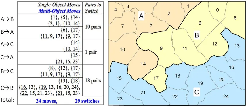
One of the major contributions of the new method is that it analyzes the contiguity relationship among objects in each district and efficiently identifies all possible moves along the border, including both single-object moves and multiple-object moves (as shown in Figure 3.1). Each move modifies the district boundary by moving an object (or multiple objects) to the neighboring district or switching objects between neighboring districts. Each move maintains all considered constraints such as geographic contiguity. Existing approaches can only allow single-object moves or switches while the new approach also allows multi-object moves.

Figure 3.1 Multi-object moves under the contiguity constraint.

In the new approach, if an object on the border between two districts cannot move due to the contiguity constraint, the method finds a minimal set of objects that will move

(31)

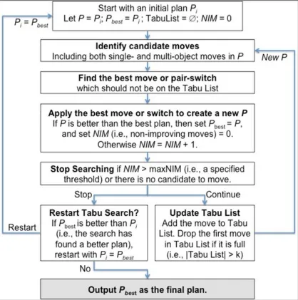
move the object (or polygon) 9 from district B to A, the contiguity of the district B will be broken. In the new method, object 9 and object 17 will move together. This new moving strategy is then combined with the Tabu search heuristics to enable a new optimization algorithm, as shown in Figure 3.2.

(32)

Figure 3.2 shows an overview of the new optimization algorithm, which is a Tabu search combined with the new contiguity-enforcing moving strategy. Tabu search methods have been used in many different applications and been shown to outperform alternative approaches (Glover 1990, Battiti and Bertossi 1999, Bozkaya et al. 2003). The algorithm progressively improves the quality of an initial plan by iteratively moving objects from one district to another. First, candidate moves are identified (including both single-object and multi-object moves). Second, the best move among them is identified and applied. The moved objects will be placed on the Tabu list for a certain period and cannot be moved again during that period, which is the key strategy in the traditional Tabu search heuristic. After each move, the list of candidate moves will be updated, and the best will be found and moved again. This process repeats until a stopping condition is met. Below I will explain the key steps in the algorithm in detail.

3.2.1 Initialization under contiguity constraint

(33)

3.2.2 Efficient algorithm for identifying multi-object moves

To efficiently identify all candidate moves (including both single-object moves and multi-object moves), I developed an efficient algorithm that can find all possible moves in linear time. Let us view the contiguity relations among spatial objects within a district as a graph G, where each spatial object is a node and two geographic neighbors are connected with an edge. If the removal of an object u from G cuts the graph into two or more disconnected components, object u is called an articulation point (a.k.a. cut point) in G. A bi-connected component is a maximal sub-graph of G that cannot be disconnected by deleting any object (Gabow 2000b). For example, the contiguity graph of district C in Figure 3.1 is shown in Figure 3.3, which has four cut points and five bi-connected components.

Algorithm 2: Initialization under contiguity constraint

Input: S: a set of spatial objects, |S| = n;

C: a n*n contiguity matrix;

r: the number of districts, 1< r << n; Steps:

1. Randomly select r objects from S, each being a district Dm, m = 1 .. r;

2. For each district Dm:

a. Randomly select one of its unassigned neighbors b (if any); b. Assign b to Dm;

(34)

First, the algorithm finds all cut points and bi-connected components in each district with a depth-first search (DFS) method, which was first described in (Tarjan 1972), and later improved by (Gabow 2000b, Tarjan 1972). The complexity of the DFS algorithm is O(n).

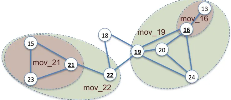
Second, the algorithm identifies a multi-object move for each cut point. Figure 3.4 shows an example and Algorithm 3 shows the algorithmic steps. By definition, bi-connected components (BCCs) are bi-connected only through cut points. If we view each BCC as a single “object”, the contiguity graph becomes a spanning tree, with cut points as the connecting “edges”. A BCC is a leaf in this tree if it only connects to one cut point (such as bcc_1 and bcc_5 in Figure 3.3). Since the removal of a cut point can cut a graph into two or more components, our strategy is to let the largest component represent the district and combine other components with the cut point to make a multi-object move. The size of a component can be defined as the number of spatial objects it contains or by other quantitative measures (such as the total population). The algorithm starts from a leaf BCC and traverses the tree from bottom up to find all multi-object moves. During the scan, the attribute values within a object move are aggregated so that each multi-object move becomes a new “multi-object”. Aggregating information within a multi-multi-object move speeds up the search for the best move since it does not need to visit all objects in each multi-object move.

(35)

object 14 in A) may move to different neighboring districts (e.g., B or C), which are viewed as two different candidate moves. The list of candidate moves is updated after making a move (and thus creating a new plan), which is repeated many times in the optimization process (Step 2 in Algorithm 1).

Figure 3.3 The contiguity relationship among the spatial objects in the district C in Figure 3.1. Neighbors are connected with edges, cut points are underlined, and dash-line ellipses show five bi-connected components.

(36)

Algorithm 3: Identifying multi-object moves

Input:

Sd: the set of spatial objects in a district d;

Cd: a contiguity matrix of the objects in Sd;

Ad: attribute vector for each object in Sd;

Steps:

CompositeMoves = ; LeafBCC = ;

1. Find all cut points and biconnected components with DFS (Sd, Cd). (See

(Gabow 2000a) for the details of the DFS algorithm.)

bcc.CPT: the set of cut points that a biconnected component bcc contains;

cpt.BCC: the set of biconnected components that a cut point cpt belongs to;

cpt.maxC = , which will keep the largest component for cpt;

cpt.restC = ; which will keep the union of other components of cpt; 2. For each biconnected component bcc:

If (|bcc.CPT| = 1): add bcc to LeafBCC; 3. Repeat the following steps until LeafBCC is empty;

bcc = next biconnected component in LeafBCCs;

cpt = the only cut point in bcc.CPT; i. If size(bcc)> size(cpt.maxC):

cpt.restC = cpt.restC cpt.maxC;

cpt.maxC = bcc;

Else: cpt.restC = cpt.restC bcc; ii. Remove bcc from cpt.BCC;

iii. If |cpt.BCC|=1 and size(cpt.maxC) < size(Sd)–size(cpt.maxC 

cpt.restC) + 1

cpt.restC = cpt.maxC cpt.restC;

bccR = the only remaining biconnected component in cpt.BCC;

cpt.BCC = ;

Remove cpt from bccR.CPT; If (|bccR.CPT| = 1):

Add bccR to LeafBCC; iv. If cpt.BCC = :

cpt = aggregation of the vectors Ad in cpt.restC;

(37)

3.2.3 Efficient evaluation of candidate moves

Based on a given objective function f, each candidate move m is given a score δm,

which is the difference in the overall objective value caused by the move. In other words,

δm = f (P) – f (Pm), where P is the current plan and Pm is the new plan after making the

move m. The move with the largest score is the best move (assuming the objective function is to be minimized). To achieve the best possible efficiency, the score for each move is calculated based on its aggregated attribute values and the aggregated information of the two involved districts. This strategy is called “dynamic scoring” (Altman and McDonald 2009). For example, given two districts A and B, and a set of candidate moves between them, the aggregated attribute values for each district may include its total population and dissolved shape boundary, which depend on the chosen set of optimization criteria. By aggregating data to districts it allows fast calculation of the score for each move without going through the entire dataset repeated and thus greatly improves efficiency. As such, it can calculate scores of all moves and find the best move in linear time.

3.2.4 Pair switch of candidate moves

(38)

sets of polygons {2, 1} and {9, 17} can be switched to their opposite district. Not all pairs can be switched due to the contiguity constraint. For example, in Figure 3.1, object 14 and object 17 cannot be switched although each can move. This situation can be quickly identified by checking the following condition. Let M1 and M2 be two candidate moves,

B1 and B2 be the boundary shared by each move with their destination district,

respectively. Let Bs be the shared boundary between M1 and M2. If B1  Bs or B2  Bs,

then we cannot switch the two moves.

3.2.5 Efficient evaluation of pair switches

(39)

number of moves in A and B. The best move identified in Section 3.2.3 is compared with the best switch identified here to determine which the overall best move is.

3.2.6 A new Tabu search algorithm

What makes the Tabu search heuristic unique is its short-memory strategy to avoid repeating the search paths that are already investigated and thus may force the search to escape local optima. Specifically, the search process uses a Tabu list to remember the most recent moves, which are prohibited to move again until they are removed from the list. The length of the Tabu list (k—the number of prohibited moves) is

normally much smaller than the data set size (n). In our experiments, k = 0.08n. A Tabu search allows non-improving moves, i.e., it is acceptable that the best move does not improve the objective value. By allowing non-improving moves, it hopes to escape a local optimum and eventually found a better solution. The search stops when the number of consecutive non-improving moves exceeds a threshold (maxNIM). In our experiments, we set maxNIM = 3n.

(40)

graph partitioning (Kernighan and Lin 1970) and has been used in many optimization problems applications such as complex network analysis (Newman 2006a).

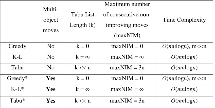
Moreover, by turning on and off new our contiguity-enforcing approach (which allows multi-object moves, as explained in Section 3.2.2), the algorithm presented in Figure 3.2 can be configured to become six different methods, as summarized in Table 3.1. If multi-object moves are not allowed (i.e., without our new approach), we have three traditional trajectory-based optimization methods: local greedy search, Kernighan–Lin (K-L) algorithm, and Tabu search. If our new contiguity-enforcing approach is integrated to allow multi-object moves, we have three new optimization methods: Greedy*, K-L*, and Tabu*, where the star (*) indicates the capability of multi-object moves. Our experiments show that each of the three new methods significantly outperforms its traditional version by a large margin and yet remains efficient.

Table 3.1 Different optimization methods.

Multi-object moves

Tabu List Length (k)

Maximum number of consecutive non-improving moves

(maxNIM)

Time Complexity

Greedy No k = 0 maxNIM = 0 O(mnlogn), m<<n K-L No k = ∞ maxNIM = ∞ O(mnlogn) Tabu No k << n maxNIM = 3n O(mnlogn) Greedy* Yes k = 0 maxNIM = 0 O(mnlogn), m<<n

(41)

3.2.7 Computational complexity

The overall complexity of the optimization method is O(mknlogn), where m is the number of criteria considered, k is the number of iterations during Tabu search, and n is the number of spatial units. Since m is generally small, k and n are the determining factors.

3.3Optimization strategies for different types of criteria

Different types of criteria can be used in the spatial optimization algorithm introduced in Section 3.2. A specific redistricting task may consider multiple criteria and give each criterion a weight. The objective function f is the weighted combination of measures of the selected criteria:

𝑓 = ∑𝑘_𝑐=1𝑤_𝑐𝑚_𝑐 (3.1)

where wc is the weight for criterion c, mc is the measure of criterion c, and k is the

number of selected criteria. Note that the measures are all transformed and normalized so that a smaller measure value means a better quality. One of the main steps in the optimization process is to find the best move among the candidate moves based on the objective function. To achieve an overall efficiency for the algorithm, different types of criteria may need different optimization strategies, which I will explain below.

3.3.1 Geographic constraints

(42)

an undirected graph. Each unit is a vertex, and two neighboring units are connected by an edge. The contiguity graph is used in the whole optimization process to make sure the generated regions are contiguous. Particularly, the identification of candidate moves, as introduced in Section 3.2, heavily rely on the contiguity graph to achieve high efficiency in finding all possible moves in a linear time.

3.3.2 Balance of district sizes

Balance of district sizes is one of the most common criteria for redistricting problems. In optimizing measures for balanced sizes, the pair switching strategy in Section 3.2.3 is very important. The balance of district sizes is normally measured by a “deviation” (Dev) value—the sum of absolute differences between each district’s actual size (pi) and its ideal size, which is the total size (P) divided by the total number of

districts r.

𝐷𝑒𝑣 = ∑ |𝑝𝑖 − 𝑃 𝑟| 𝑟

𝑖=1 (3.2)

In some redistricting problems, the ideal size can be different for each district. For example, in school redistricting, the ideal size depends not only on the total student population and the total number of districts, but also on the capacity of each school (ci).

𝐷𝑒𝑣 = ∑ |𝑝_𝑖 − 𝑐𝑖𝑃 ∑𝑟𝑖=1𝑐𝑖

| 𝑟

𝑖=1 (3.3)

(43)

𝐷𝑒𝑣 = ∑ ∑𝑚𝑔=1𝑤𝑔|𝑝𝑖𝑔− 𝑐𝑖𝑔𝑃𝑔 ∑𝑟𝑖=1𝑐𝑖𝑔

| 𝑟

𝑖=1 (3.3)

where g is the grade, m is the total number of grades, and wg is the weight for grade g.

3.3.3 District-specific targets

Some criteria are only evaluated for certain districts. For example, in political redistricting, it is required for certain states (e.g., South Carolina) that there must be one or more majority-minority districts, in which the minority groups (e.g., Black population) make up a majority of the population. So the percentages of different racial groups will only be evaluated for some of the districts, and different targets can be set for different districts. In the initialization process, the targets are set for districts whose initial measures are close to the targets. The optimization algorithm calculates the measures for only the districts where the targets are set.

3.3.4 Compactness

Certain redistricting tasks require that the shape of each district should be as compact (or simple) as possible. For example, as a means to prevent gerrymandering, the constitution of Iowa specifically requires that the political redistricting process must consider compactness of each district. One commonly used compactness measure is the Polsby-Popper index, which divides the area ( ) of the district by the area of a circle

with the same perimeter ( ) as that of the district (Polsby and Popper 1991). This measure ranges from 1 (perfect circle) to zero. This measure can be part of the overall objective function. There is no specific optimization strategy for the compactness measure.

i



i

(44)

𝐶𝑜𝑚𝑝𝑎𝑐𝑡𝑛𝑒𝑠𝑠 =1 𝑟∑

4𝜋𝛼𝑖 𝜌𝑖2 𝑟

𝑖=1 (3.4)

3.3.5 Travel distance

For redistricting problems such as school redistricting and business service area redistricting, travel distance is an important factor to be considered. For example, the average travel distance to school needs to be minimized for school redistricting. The travel distance is calculated for every pair of the unit and the fixed location (e.g. school), and a distance matrix is created. The average travel distance is constantly updated using the distance matrix in the optimization process. Since the average distance can be affected by a few large distances, an average distance order measure can be used as a proxy. The distances from all units to a fixed location are ordered, and each distance is assigned an order number starting from 1. The optimization algorithm tries to minimize the average distance order measure, and tries to assign a unit to its closest fixed location.

3.4Conclusion

(45)

CHAPTER 4 PERFORMANCE EVALUATION, USER INTERACTION, AND

COMPUTATIONAL SOLUTION FOR LARGE DATASETS

The key contributions of the new spatial optimization method include (1) computational efficiency—the new optimization strategies significantly improve the computational efficiency of existing methods and thus enable applications with redistricting optimization while allowing real-time user interaction, (2) optimization quality—the method reliably achieves much higher optimization quality than existing methods, and (3) flexibility—with both efficiency and quality the method provides a flexible framework to consider different sets of criteria and produce results that meet practical needs.

(46)

new method presented in this dissertation is already significantly faster than existing methods, it still needs further computational solutions to handle large datasets, such as tens of thousands spatial objects, to produce optimization results that meet practical requirements.

4.1Performance evaluation with case studies

Redistricting problems are encountered in many different application domains including political districting, school districting, sales districting, and community structure detection. The primary difference among these application problems is the set of criteria and constraints being considered in the optimization process. The new method introduced in Chapter 3 can consider different sets of criteria and constraints. I carried out several case studies to demonstrate and evaluate the method.

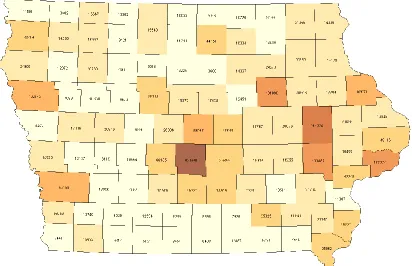
4.1.1 Iowa congressional redistricting

(47)

Figure 4.1 Iowa counties and their population (2010 census).

1) Optimizing population equality only

The first experiment considers only the population equality criterion. Population equality is measured with a “deviation” value (PopDev), which is the sum of absolute differences between each district’s actual population and its ideal population, which is the total size divided by the total number of districts. For Iowa, the ideal population for each district is 761588 or 761589 (as 3,046,355 / 4 = 761588.75, which is used internally in the algorithm as the ideal population).

(48)

optimization methods, while Greedy*, K-L*, and Tabu* are the new optimization methods developed in this research with the new contiguity-enforcing and optimization strategies. Specifically, Tabu* is the chosen new method in this research as it consistently achieves the best performance across all experiments.

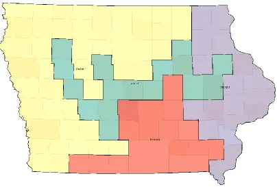
Each method generates 1000 plans on an i7-3770 (3.40 GHz) machine. The summary statistics of the 1000 PopDev values for each method are shown in Table 4.1, which show that each of the new optimization methods significantly outperforms its traditional version. Particularly, the Tabu* method (i.e., the new optimization method of this research) reliably achieves the best performance, with average = 133 and standard deviation = 68, which statistically outperforms all other methods. The best plan of the 1000 results found by Tabu* by only optimizing the population equality criterion has a PopDev value of 4.5, which is probably the global optimal solution. The theoretical global optimal value for PopDev is 1.5 since the ideal population (761588.75) is not a whole number. Figure 4.2 shows the map for this plan. The computational time for Tabu* in this experiment is 33 seconds for generating 1000 plans, i.e., it takes 0.03 second to optimize each plan.

(49)

Table 4.1 Evaluations with Iowa data for optimizing population equality (PopDev).

1000 Runs Traditional optimization methods New methods

Greedy K-L Tabu Greedy* K-L* Tabu* Min 646 421 109 81 33 4.5 5% 3937 1432 650 559 165 51 Q1 (25%) 7037 3184 1364 1400 369 89

Median (50%) 9531 4684 2149 2697 579 133

Q2 (75%) 12546 6436 3590 4881 976 181 95% 18372 9092 7020 11036 1854 253 Max 169308 87299 70167 70167 8224 497

Standard Deviation 8051 4077 3066 4611 668 68

(50)

2) Optimizing both population equality and shape compactness.

The second experiment considers both population equality and compactness. As explained in Chapter 3, the compactness is measure with the Polsby-Popper index, which divides the area of the district by the area of a circle with the same perimeter as that of the district (Polsby and Popper 1991). This measure ranges from 1 (perfect shape) to zero.

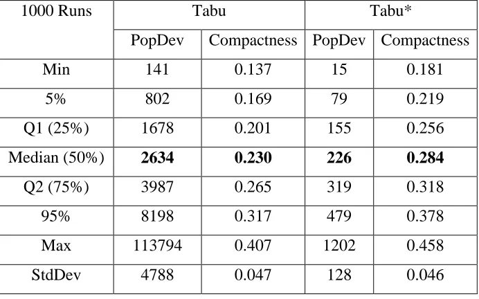
In this experiment we focus on the difference between Tabu and Tabu*. Each method generates 1000 plans on an i7-3770 (3.40 GHz) machine. The summary statistics of the two sets of measure values for each method are shown in Table 4.2. Note that a larger value for compactness means a more compact shape, while a smaller value for PopDev means better population equality. Internally in the algorithm, these measures are transformed and normalized before being combined into an objective function. The results show that Tabu* again significantly outperforms its traditional version.

Table 4.2 Evaluation with Iowa data, optimizing population equality and compactness 1000 Runs Tabu Tabu*

PopDev Compactness PopDev Compactness Min 141 0.137 15 0.181

5% 802 0.169 79 0.219 Q1 (25%) 1678 0.201 155 0.256 Median (50%) 2634 0.230 226 0.284

(51)

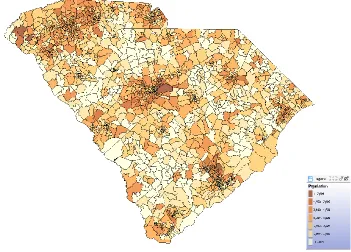
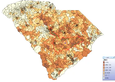
4.1.2 South Carolina congressional redistricting

The criteria for congressional redistricting in South Carolina include population equality, contiguousness, compactness, majority-minority districts, and communities of interest. County boundaries, municipality boundaries, and voting precinct boundaries should be considered when practical and appropriate, since they are considered as one kind of evidence of communities of interest. In this research, voting precincts are used as the spatial units. South Carolina has 2122 voting precincts (Figure 4.3), which are to be divided into 7 congressional districts based on 2010 census data. The total population of South Carolina is 4,625,364 and therefore the ideal population for each district is 660,766. In calculating the PopDev measure, the value 4,625,364 / 7 = 660766.285714 is used. The theoretical global optimal value is 2.857142.

(52)

1) Optimizing population equality only

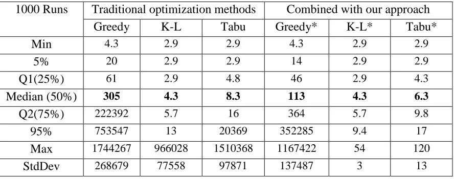
The South Carolina data set is much larger than the Iowa data set in terms of the number of spatial objects (units) and thus requires more computational time. However, more spatial objects actually make it easier to find the global optimum when only considering population equality. The best results from 1000 runs of the three traditional optimization methods are comparable with those of the new optimization methods integrated with the new methods, and except Greedy, all methods found many solutions to achieve the theoretical global optimal value. The new methods are more significantly more robust and consistent, evidenced by their very small standard deviation values. It is interesting to notice that the K-L method (which can be considered a special case of Tabu with a Tabu list of infinite length) and its new extension K-L* slightly outperform Tabu and Tabu*, respectively. This provides important insights on the configuration of Tabu parameters in relation to data size, which is a future direction for this research.

Table 4.3 Evaluations with South Carolina data, optimizing population equality only.

Values are rounded a whole number or keeping one decimal digit for values less than 10. The theoretical global optimal value is 2.857142, which is rounded to 2.9 in the table.

1000 Runs Traditional optimization methods Combined with our approach Greedy K-L Tabu Greedy* K-L* Tabu* Min 4.3 2.9 2.9 4.3 2.9 2.9

5% 20 2.9 2.9 14 2.9 2.9

Q1(25%) 61 2.9 4.8 46 2.9 4.3

Median (50%) 305 4.3 8.3 113 4.3 6.3

Q2(75%) 222392 5.7 16 364 5.7 9.8

95% 753547 13 20369 352285 9.4 17

Max 1744267 966028 1510368 1167422 54 120

(53)

2) Optimizing population equality, compactness, and majority-minority districts In this case study, three criteria are considered: population equality, district compactness, and creating a majority-minority district in which the minority population is the majority. In order to create a majority-minority district, a community of interest (COI) is outlined on the map by the user, which contains precincts with a large percentage of minority population (Figure 4.4). The optimization method will take this COI as input, optimize a district containing the COI to generate a majority-minority district, and in the meantime optimize all chosen criteria to generate a plan of seven districts.

Figure 4.4 A user-drawn community of interest (COI).

(54)

advantage of the new method is that it is flexible to consider various criteria, allows interactive user inputs and visual inspection (which will be elaborated in Section 4.2).

Figure 4.5 A plan with a majority-minority district.

4.1.3 School redistricting

School redistricting is different from political redistricting in two important aspects. First, the optimization criteria to be considered are quite different. Common criteria and constraints considered in school redistricting are listed below, among which the first two are considered as constraints. Second, each district is constructed around a fixed location, i.e., school. This location is not only important for certain criteria such as distance to school but also critical in determining the district boundary, which should contain the location.

(55)

 Each district contains one and only one school

 Balance the number of students to school capacity (for each grade)

 Shape compactness

 Average distance to school

 Existing school district boundaries

In this case study, we use a real-world scenario. Prince William County, Virginia has used the redistricting method and system developed in this research to redraw the boundaries of the school districts for its16 middle schools (Figure 4.6). All the six criteria listed above are used. Particularly, the projected student populations for each grade in future years are considered in evaluating the balance between student population and school capacity for each district. The choice, configuration, and weight of each criterion can be set interactive with visual interfaces (which is introduced in Section 4.2).

(56)

Figure 4.7 shows one of the school redistricting plans, which achieves very good scores across the chosen criteria, much better than one could achieve with a manual approach as used in most of the current practices of school redistricting. Most importantly, the new method and its implemented system give general users the immense power to construct redistricting plans and participate in the redistricting process, which is impossible with existing methods and available software tools.

(57)

4.2Visual interface and user interaction to integrate human inputs

4.2.1 Subjective criteria

There are vague and subjective criteria that cannot be clearly defined, such as preserving communities of interest. Different people may have different understandings of “communities”, for which local knowledge is needed. For such vague and subjective criteria, visual interface is needed to dynamically integrate human judgments with the computational method. For example, the user may draw several areas to indicate communities of interest to be preserved. Then the algorithm will optimize selected criteria under these constraints, i.e., each user-drawn community will not be split during the Tabu search. Figure 4.8 (Maps D to F) shows three selected results with such user provided constraints. For example, Map D and Map E are two different plans for the same set of user drawings, while Map F is a plan for a different set of drawings.

(58)

Figure 4.8 Iowa congressional redistricting with the 2000 census data. Maps (A-C) show three selected results with the new method without user drawing. Maps (D-F) show three selected results with user drawings (indicated by the green semi-transparent areas). PopDev is the measure for equal population, which is the total deviation between district population and its target population, which is the smaller the better.

4.2.2 Visual interface and user interaction

(59)

Figure 4.9 The redistricting system, iRedistrict, based on the new optimization method.

(60)

1) Mapping

The user can choose the variable to be classified for the unit layer and create a choropleth map. The number of classes and the color scheme can also be defined. The labels can be shown if needed. A legend panel is shown to display the color and the break for each class. This map can help the user understand the distribution of the selected variable, which in turn facilitates the understanding of the optimizaiton quality for the specific plan shown in the map.

(61)

2) Community of Interest (COI)

A COI tool bar can be shown if the user wants to draw on the map to express constraints. It’s a free drawing tool, which means the user can draw any type of polygon shapes. The user can click on the map to add a vertex, and double click to close the polygon. The unit objects intersected by the polygon will be considered as a COI, and thus won’t be broken during the optimization process. The COI will be assigned a name and added to the COI dropdown list. The user-drawn COIs can be saved as a shapefile and loaded back later. Actually, the user can load any shapefile and choose some polygons from it to be COIs.

3) Algorithm configuration and execution

The user can enable the required criteria for redistricting and set the parameter for them such as the weight and the threshold (Figure 4.10(C)). More criteria can be added by clicking the “+” button on the criteria tab row. The user can choose the type of the criterion and input a unique name for it. A new tab for the added criterion will be shown. Unused criteria can also be removed. In this way, the user can easily define the required criteria for different redistricting problems.

The user can then configure the optimizaton algorithm, the number of districts, and the number of plans to be generated. By clicking the “run” button, the chosen optimization algorithm will be run with the configured criteria and constraints to generate the required number of redistricting plans.

4) Visual examination and comparison of alternative plans

(62)

of the two most common critera: popualtion equality and compactness. By default, the plan list is sorted by the combined score of all selected criteria (i.e the value of the objective function). The user can sort the plan list by the score of one criterion by using the “sorted by” dropdown list. The scatter plot shows the distribution of the scores of two criteria (population equality and compactness by default). The user can choose the criterion for each axis and compare the scores of different plans. The plan list and the scatter plot are linked, which means that clicking a plan on the list will highlight the plan on the scatter plot , and vice vesa. When a plan is clicked on the list or the scatter plot, the map will be updated to show its districts, and the report table in the report panel will be updated to show the attributes of the districts. The user can configure the attributes to be shown in the report table.

5) Managing plans

After examining and comparing the alternative plans, the user can add desired plans to the selected plan list (Figure 4.10(E)). The user can rename the selected plans. The labels of the districts in a selected plan can also be changed. The selected plans can be saved as a csv file, in which each column represents a plan. The saved csv file can be loaded back and added to the plan list. The current selected plan can also be saved as a shapefile of all districts, or several shapefiles each of which represents a district.

6) Locking districts

Sometimes an alternative plan is not good enough, but some of the districts are pretty good. In this case, the user can use the “lock” tool to lock the good districts and run the optimization algorithm again. The locked districts will be kept in the generated plans.

(63)

An “edit” tool is provided to change an alternative plan based on the user’s judgement. The user can drawn an polygon (like drawing COIs) to select some units, and a popup menu is then displayed to show a list of the districts that are neighboring these units. The user can choose the district these units will be moved to. If this change breaks the spatial contiguity, the user will be warned. The scatter plot, the plan list, and the report table will be updated after the change. If the user thinks the change is good, editing mode can be stopped and the change can be saved. The plan can be reverted to the previous state if the change is not good.

4.3Computational solutions for handling large data volume

As explained in Chapter 3, the overall complexity of the optimization algorithm is

O(mknlogn), where m is the number of criteria considered, k is the number of iterations during Tabu search, and n is the number of spatial units. To handle large datasets (e.g., n > 10,000), several strategies are developed by reducing k and/or n while not significantly sacrificing optimization quality.

4.3.1 Mega districts

(64)

California needs 53 congressional districts. Keep in mind, as required by the redistricting rule, larger units should be used whenever possible. The user will first divide the state into a small number (of the user’s choice) of mega districts at the county level. The equal-population rule requires that the population of each mega district should be as close as possible to a whole number of ideal district population. With the interactive process, a list of mega-district plans can be generated. If none of them sufficiently meets the equal population requirement, the user can break one or several counties into smaller units (such as VTDs) and optimize again. Once satisfied, the user then partitions each mega district separately. Since human’s understanding of space is inherently hierarchical (Hirtle and Jonides 1985, Kuipers 2000), to divide a large state into many districts, it is more intuitive to take such a hierarchical process.

1) Mega district generation

The number of mega districts is determined by the defined max unit number of a mega district. The mega districts are generated using the same redistricting algorithm, but only the population and the shape compactness are considered. The target population for a mega district is a whole number of ideal district population so that the sum of the district numbers in mega districts is equal to the original required number of districts.

2) Plan generation

(65)

Algorithm 4: Mega districts

Input:

n: the number of units in the whole area;

totalPop: the total population of the whole area;

r : the number of required districts;

ki: the number of required districts in the ith mega district;

Steps:

1. Divide the whole area into mega districts

i. Set Nmax to be the maximum number of units in a mega district;

ii. Set the number of mega districts = 𝑀𝑖𝑛(𝐶𝑒𝑖𝑙(𝑛 / 𝑁_𝑚𝑎𝑥), 𝑟/2) , where Ceil() returns the smallest integer that is greater or equal to the input value. This makes sure the number of units in each mega district is less than Nmaxand each mega district has at least two districts;

iii. Set 𝑘_𝑖 = 𝑟

𝑚(𝑖 = 1, 2, … , 𝑟) ;

iv. Repeat the following until ∑𝑟𝑖=1𝑘𝑖 = 𝑟 : ki++;

i++;

v. SET the target population for the ith mega district 𝑡𝑎𝑟𝑔𝑒𝑡𝑃𝑜𝑝𝑖 = 𝑘𝑖 ∗ 𝑡𝑜𝑡𝑎𝑙𝑃𝑜𝑝/𝑟;

vi. Create m mega districts using the redistricting algorithm with the equal population and shape compactness criteria;

2. Run the redistricting algorithm in each mega district

i. Split the original data set into each mega district;

ii. Set the criteria for each mega district;

iii. Create a certain number of sub-plans with ki districts for the ith mega

district;

iv. Select the top sub-plans based on the measure;

3. Combine the sub-plans in mega districts to form the final plans for the whole area

i. Select one sub-plan in each mega district;

(66)

4.3.2 Clustering

Clustering is a bottom-up process to decrease the number of units in the redistricting optimization process. The number of clusters is determined by a defined max population of a cluster. First, each unit is considered as a cluster. Then, a cluster is selected randomly, and its one neighbor is temporarily added to it. The measure of the new cluster is calculated and recorded, and the cluster is then reset. The neighbor that results in the best measure will be permanently added to the cluster. The process is repeated until there is no cluster to be merged under the max population constraint. These clusters are used instead of the original units in the redistricting process.

Algorithm 5: Clustering

Input:

n: the number of units in the whole area;

totalPop: the total population of the whole area; Cmin: the minimum number of clusters;

maxClusterPop : the maximum population of a cluster (totalPop/C_min); Steps:

1. Each unit is considered as a cluster at the beginning; 2. Repeat the following steps until no clusters can be merged:

i. Randomly select a cluster.

ii. For each neighbor of the cluster:

a. Temporarily add this neighbor to the cluster;

b. If the population of the new cluster < maxClusterPop: Calculate the measure of the new cluster

(67)

(A) (B)