Multi-objective Optimization of Tube Hydroforming Using Hybrid Global and Local Search

University of Windsor University of Windsor

Scholarship at UWindsor

Scholarship at UWindsor

Electronic Theses and Dissertations Theses, Dissertations, and Major Papers

2010

Multi-objective Optimization of Tube Hydroforming Using Hybrid

Multi-objective Optimization of Tube Hydroforming Using Hybrid

Global and Local Search

Global and Local Search

Honggang An

University of Windsor

Follow this and additional works at: https://scholar.uwindsor.ca/etd

Recommended Citation Recommended Citation

An, Honggang, "Multi-objective Optimization of Tube Hydroforming Using Hybrid Global and Local Search" (2010). Electronic Theses and Dissertations. 454.

https://scholar.uwindsor.ca/etd/454

MULTI-OBJECTIVE OPTIMIZATION OF TUBE HYDROFORMING USING HYBRID GLOBAL AND LOCAL SEARCH

by Honggang An

A Dissertation

Submitted to the Faculty of Graduate Studies

through Mechanical, Automotive and Materials Engineering in Partial Fulfillment of the Requirements for

the Degree of Doctor of Philosophy at the University of Windsor

Windsor, Ontario, Canada

Declaration of Co-Authorship / Previous Publication

I. Co-Authorship Declaration

I hereby declare that this dissertation does not incorporate material that is result of joint research. In all cases, the key ideas, primary contributions, experimental designs, data analysis and interpretation, were performed by the author, and Dr. D. E. Green and Dr. J. Johrendt as advisors.

I certify that, with the above qualification, this dissertation, and the research to which it refers, is the product of my own work.

II. Declaration of Previous Publication

This dissertation reflects the content of 5 original papers that have been previously published/submitted for publication in peer reviewed journals and conferences, as follows:

Dissertation

Chapter Publication title/full citation

Publication status

Chapter 4 H. An, D.E. Green, J. Johrendt, Multi-objective optimization and sensitivity analysis of tube hydroforming

simulations, Int. J. Advanced Manufacturing

Technology,DOI:10.1007/s00170-009-2505-x (2010)

Published

Chapter 5 H. An, D.E. Green, J. Johrendt, Optimal load path design for tube hydroforming using hybrid constrained MOGA and local search, Advanced Engineering Informatics

Submitted

Chapter 5 An, H., Green, D.E., and Johrendt J. A global optimization of load path design for tube hydroforming applications using MOGA, IDDRG, June, Golden, CO, USA, p307-318 (2009)

Published

Chapter 5 Honggang An, Green, D.E., Johrendt J. and K. Hertell, Inverse Analysis in Hydroforming of a Refrigerator Door Handle Using MOGA, Accepted by NUMIFORM2010, Pohang, Korea. June 2010.

Published

Chapter 6 An, H., Green, D.E., and Johrendt J. Optimization of tube hydroforming using pulsating internal pressure,

Proceedings of Materials Science & Technology (MS&T),

October 25-29, 2009, Pittsburgh, Pennsylvania, USA, p2321-2332 (2009)

I certify that I have obtained written permission from the copyright owner(s) to include the above published material(s) in my dissertation. I certify that the above material describes work completed during my registration as graduate student at the University of Windsor.

I declare that, to the best of my knowledge, my dissertation does not infringe upon anyone’s copyright nor violate any proprietary rights and that any ideas, techniques, quotations, or any other material from the work of other people included in my dissertation, published or otherwise, are fully acknowledged in accordance with the standard referencing practices. Furthermore, to the extent that I have included copyrighted material that surpasses the bounds of fair dealing within the meaning of the Canada Copyright Act, I certify that I have obtained a written permission from the copyright owner(s) to include such material(s) in my dissertation.

ABSTRACT

An investigation of non-linear multi-objective optimization is conducted in order to define a set of process parameters (i.e. load paths) for defect-free tube hydroforming. A generalized forming severity indicator that combines both the conventional forming limit diagram (FLD) and the forming limit stress diagram (FLSD) was adopted to detect excessive thinning, necking/splitting and wrinkling in the numerical simulation of formed parts.

In order to rapidly explore and capture the Pareto frontier for multiple objectives, two optimization strategies were developed: normal boundary intersection (NBI) and multi-objective genetic algorithm (MOGA) based on the concept of “dominated solutions”. The NBI method produced a uniformly distributed set of solutions. For the MOGA method, a stochastic Kriging model was used as a surrogate model. Furthermore, the constraint-handling technique was improved, Kriging model updating was automated and a hybrid global-local search was implemented in order to rapidly explore the Pareto frontier.

DEDICATION

To

My family and

ACKNOWLEDGEMENTS

I am indebted to my supervisor, Dr. Daniel E. Green and co-supervisor, Dr. Jennifer Johrendt, for their distinguishing guidance through the research work and their help in setting up a positive start for my research and engineering career in Canada.

Also I am grateful to Dr. P. Bieling, formerly from Valiant Machine & Tool Inc., for his advice during this work. Thanks are also granted to Mr. K. Hertell, from Schuler Inc., for providing data and advice for the industrial case study. The author would like to thank Dr. T. B. Stoughton for valuable discussions during the NADDRG 2008 Spring conference.

All the committee members, Dr. W. Altenhof, Dr. N. Zamani and Dr. F. Ghrib, are gratefully acknowledged for their advice and support during my research. In particular, I am grateful to Dr. W. Altenhof for providing continuous support and advice in numerical simulation, as well as quick response at any time.

The authors would like to acknowledge the financial support of the Natural Sciences and Engineering Research Council of Canada (NSERC) , the Ontario Graduate Scholarship and the Ontario Graduate Scholarship in Science and Technology.

My family's support is always the motivation to my study. I am thankful to my parents and my wife Carol.

TABLE OF CONTENTS

Declaration of Co-Authorship / Previous Publication ... iii

Abstract ... v

Dedication ... vii

Acknowledgements ... viii

List of Tables ... xiii

List of Figures ... xv

List of Abbreviations ...xix

Nomenclature ...xxi

Chapter 1 INTRODUCTION AND PROBLEM STATEMENT ...1

1.1 Introduction ...1

1.1.1 Tube hydroforming and its advantages ...1

1.1.2 Tube failure in tube hydroforming ...2

1.1.3 Evaluation of forming severity in tube hydroforming (FLD and FLSD) .2 1.1.4 Multi-objective optimization ...4

1.2 Problem statement ...6

1.3 Dissertation Organization ...7

Chapter 2 LITERATURE REVIEW ...8

2.1 Tube hydroforming ...8

2.1.1 Introduction ...8

2.1.2 Examples of hydroforming in the automobile industry ...9

2.2 Conventional design method of loading path ...10

2.2.1 Analytical method ...11

2.2.2 Finite Element Method ...15

2.3.1 Classical optimization algorithms ...17

2.3.2 Intelligent optimization algorithms ...21

2.3.3 Summary of classical and intelligent methods...25

2.3.4 Multi-objective optimization ...25

2.3.5 Meta-model based multi-objective optimization ...32

2.3.6 Literature of multi-objective optimization in tube hydroforming...40

2.4 Review of available software in metal forming optimization...41

Chapter 3 A HYBRID FORMING SEVERITY INDICATOR FOR

TUBE HYDROFORMING SIMULATION ... 43

3.1Failure modes of tube hydroforming ...43

3.2Strain based forming limit diagram ...46

3.2.1 Path dependence of strain-based forming limits ...48

3.3Stress-based FLD ...50

3.4General objectives for defect-free tube hydroforming ...51

Chapter 4 MULTI-OBJECTIVE OPTIMIZATION AND SENSI-TIVITY

ANALYSIS FOR TUBE HYDROFORMING USING NORMAL

BOUNDARY INTERSECTION ... 55

4.1Introduction ...55

4.2Response surface methodology...57

4.3Normal boundary intersection...58

4.4A RSM based optimization algorithm for tube hydroforming ...61

4.5Implementation ...63

4.6Application to straight tube hydroforming ...63

4.6.1 Objectives and optimization model for tube hydroforming with square die ...64

4.6.2 Finite element simulation with LS-DYNA® ...65

4.6.3 Virtual experiment design of loading path ...67

4.6.5 Validation with LS-OPT® 4.0 ...79

4.6.6 Conclusions ...81

Chapter 5 LOADING PATH DESIGN USING MULTI-OBJECTIVE

GENETIC ALGORITHM FOR A STRAIGHT TUBE AND AN

INDUSTRIAL PART ... 83

5.1Kriging metamodel ...83

5.2MOGA and constraint handling technique ...84

5.2.1 MOGA ...84

5.2.2 Constraint handling technique ...86

5.3MOGA-I (Global Search) and MOGA-II (Hybrid Global and Local Search or H-MOGA) ...88

5.3.1 MOGA-I ...88

5.3.2 MOGA-II (H-MOGA) ...91

5.4Case study 1: Straight tube hydroforming using Algorithm I...94

5.4.1 The FE model ...94

5.4.2 Optimization procedure ...94

5.4.3 Design of experiments ...96

5.4.4 Strategy for automatic data processing ...96

5.4.5 Results ...98

5.4.6 Discussion ...99

5.4.7 Conclusions for case study 1...102

5.5Case study 2: Straight tube hydroforming considering local thinning using H-MOGA ...103

5.5.1 Design variables ...103

5.5.2 Design objective function and constraints ...103

5.5.3 Kriging surrogate model ...104

5.5.6 Results validation and discussion ...110

5.5.7 Conclusions for case study 2...112

5.6Case study 3: Inverse analysis using MOGA for hydroforming of a refrigerator door handle...113

5.6.1 Introduction ...113

5.6.2 Geometry of the tube and the die ...114

5.6.3 FEA model ...114

5.6.4 Load path design and sensitivity analysis ...116

5.6.5 Process optimization ...118

5.6.6 Inverse strategy ...120

5.6.7 Objective functions ...121

5.6.8 Optimization results for loading path ...123

5.6.9 Conclusions ...128

Chapter 6 OPTIMIZATION OF LOADING PATH IN

HYDRO-FORMING WITH PULSATING PRESSURE ... 130

6.1Introduction ...130

6.2Mechanism of pulsating hydroforming ...131

6.3Load path design for hydroforming ...132

6.4Finite element model...133

6.5Optimization procedure ...136

6.5.1 The MOGA algorithm...137

6.5.2 Mathematical model of the T-shape pulsating hydroforming...137

6.6 Results and discussion ...139

6.7Conclusions ...141

Chapter 7 LOADING PATH DESIGN IN MULTI-STAGE TUBE

FORMING ... 142

7.2Rotary-draw bending ...143

7.2.1 Factors affecting bending ...144

7.2.2 Boost method ...144

7.3Bent tube hydroforming ...145

7.4Simulation of tube bending and hydroforming ...146

7.4.1 Material properties ...146

7.4.2 Procedure for the bending ...148

7.4.3 Hydroforming simulation...150

7.4.4 Simulation results of the tube bending (strain and thickness) ...151

7.5Optimization of pre-bent tube hydroforming ...155

7.5.1 Objective functions ...155

7.5.2 Design of experiments ...157

7.5.3 Results obtained using MOGA-I ...158

7.5.4 Discussion of the stress history ...161

Chapter 8 CONCLUSIONS AND FUTURE WORK ... 167

8.1Conclusions ...167

8.2Recommendations for future work ...169

Bibliography ...170

Appendix A ...182

Appendix B ...183

Appendix C ...184

Appendix D ...187

Appendix E ...189

Publications ...191

LIST OF TABLES

Table 2.1: Number of experimental points required for experimental designs ...36

Table 4.1: Tube properties ...67

Table 4.2: L9(34) orthogonal array ...69

Table 4.3: Factor responses with L2 norm value and S/N ratio for each objective .71 Table 4.4: L18(36) orthogonal array ...72

Table 4.5: Factor responses with L2 norm and S/N ratio for each objective of the L18 orthogonal array...73

Table 4.6: Two optimum solutions obtained with the NBI method using L2 norm and FEA for verification ...76

Table 4.7: Loading path parameters for the global optimum solution ...77

Table 4.8: Comparison of objectives of final optimum (L2 norm value) and intermediate results ...77

Table 4.9: Algorithms and parameters in LS-OPT® GUI ...80

Table 4.10: Optimum results obtained using LS-OPT® (unit: mm for radius) ...80

Table 5.1: Three different load paths ...100

Table 5.2: Comparison of the forming results with different loading paths ...101

Table 5.3: Accuracy of response surface of objectives ...105

Table 5.4: The objectives of the three selected points (without units) ...106

Table 5.5: Local search result in region A ...110

Table 5.6: Local search result in region B ...110

Table 5.7: Mechanical properties and geometry of the tube ...115

Table 5.8: Comparison of the objectives for two optimum loading paths with different COF values ...124

Table 5.9: Pressure and end feed parameters for two coefficients of friction ...125

Table 6.1: Three types of pressure paths ...133

Table 6.2: Mechanical properties of the tube ...134

Table 6.3: FEA results with three load paths ...136

Table 6.4: Optimal results using MOGA with a minimum L2 norm ...139

Table 7.1: Mechanical properties of the tube ...147

Table 7.2: COF used in tube bending simulations ...147

Table 7.3: The Comparison of strain and thickness ...152

Table 7.4: Accuracy of response surface of the objectives ...158

Table 7.5: The optimal load path obtained using MOGA ...158

Table 7.6: The objectives obtained by current optimal load path ...158

Table 7.7: The parameters for local search ...163

Table 7.8: The optimal load path ...163

LIST OF FIGURES

Figure 1.1 Example of THF process window ...3

Figure 1.2 Pareto set for multi-objective optimization with two objectives (Minimizing) ...5

Fig. 2.1 Tube hydroforming process of straight tube (Courtesy of Schuler Inc.) ...8

Fig. 2.2 Typical hydroformed parts in an automobile ...10

Fig. 2.3 Load-curve for internal pressure vs. time ...13

Fig. 2.4 SF loading paths: α _{is a scale factor to increase the amount of axial feeding} ...20

Fig. 2.5 Schematic procedure of the AS ...21

Fig. 2.6 The process of the adaptive simulation ...22

Fig. 2.7 Pareto-optimal solution for two objectives...27

Fig. 2.8 Surrogate modeling philosophy ...28

Fig. 2.9 The crossover and mutation operations in EA ...30

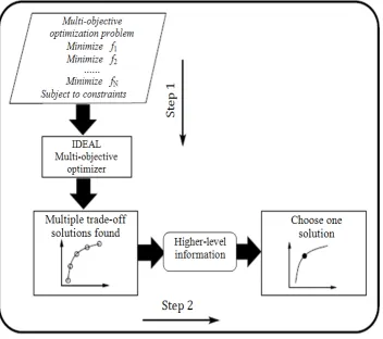
Fig. 2.10 Schematic of a two-step multiobjective optimization procedure ...31

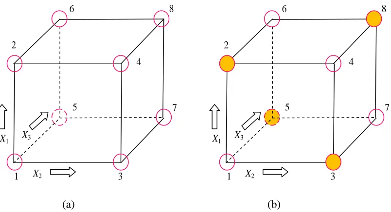
Fig. 2.11 A two level full factorial design (factors X1, X2,X3); (b) fractional design ...33

Fig. 2.12 Approximation techniques...39

Fig. 2.13 Response surface methodology (i.i.d: independent and identically distributed) ...39

Fig. 2.14 Kriging model40 Fig. 3.1 The principle of tube hydroforming: (a) original tube shape and (b) final tube shape (before unloading) ...44

Fig. 3.2 Diagram showing various failure modes in tube hydroforming ...44

Figure 3.4 Strain path-dependency of FLC (adapted from Graf and Hosford) ...49 Fig 3.5 Prestraining in biaxial tension shifts the FLC down and to the right ...49 Fig. 3.6 (a) Comparison of the as-received FLC with that after a prestrain to 0.07 strain in equibiaxial tension and (b) the corresponding FLSC in stress space.50 Fig. 3.7 Graphical interpretation of the objective functions on a) the FLD b) the FLSD ...53 Fig. 4.1 Process windows for tube hydroforming ...55 Fig. 4.2 Finding the shadow minima in step 1 (represented by two dots N and T) .60 Fig. 4.3 Finding the best set of trade-off solutions in step 2 ...60 Fig. 4.4 Metamodel based optimization...62 Fig. 4.5 Interface with FEA to calculate the objectives of necking/fracture, wrinkling and severe thinning ...63 Fig. 4.6 Location of three nodes used to measure the corner radius ...64 Fig. 4.7 One quarter of the FE model of straight tube hydroforming ...65 Fig. 4.8 Geometry of the cross-section of die and tube (RC is the final corner radius of the deformed tube) ...66 Fig. 4.9 Piecewise linear load curve for internal pressure and axial end feed displacement ...68 Fig. 4.10 Predicted strain paths in the most critical element (maximum major stress)

Fig. 5.1 (a) Schematic of the NSGA-II procedure, and (b) the crowding distance calculation ...85 Fig. 5.2 Constrained NSGA-II algorithm ...88 Fig. 5.3 Flowchart of optimization strategy using Kriging predictor for generating both new points and offsprings ...89 Fig. 5.4 MOGA ranking strategy ...90 Fig. 5.5 Flowchart of optimization strategy (a) Using Kriging predictor for generating both new points and offsprings (b) Kriging predictor used only for generating new points and FEA for offsprings ...93 Fig. 5.6 (a) One quarter of the FE model (b) Geometry of the cross-section of die and tube (RC is the final corner radius of deformed tube) ...94 Fig. 5.7 Load curve for (a) internal pressure; and (b) axial end feed displacement

Fig. 5.17 Forming process of a refrigerator door handle ...115

Fig. 5.18. Finite element mesh ...116

Fig. 5.19 Stress-strain curve (true and engineering) ...116

Fig. 5.20 Loading path design ...117

Fig. 5.21 An example of objective function and optimization variables [18] ...119

Fig. 5.22 (a) Measure of distance d1 in the lower die and (b) Measure of distance d2 in the upper die...120

Fig. 5.23 Validation of simulation by comparing the stress-strain response from FEA and extrapolated experimental data ...122

Fig. 5.24 Pareto optimal set for four objectives (f1 vs. f2, f6 and f3). (The squares show the final solution set with a constraint of maximum thickness reduction of 30%)...124

Fig. 5.25 The comparison of loading paths for two COF (0.05 and 0.1, respectively) ...125

Fig. 5.26 (a) The tube filling and the thickness distribution in a cross-section (b) The effective stress distribution and the maximum stress...126

Fig. 5.27 Comparison to the actual load path: (a) Pressure vs. time and (b) End feed vs. time ...128

Fig. 6.1 Calculated oscillation of stress components during pulsating hydroforming ...131

Fig. 6.2 Cause of uniform expansion in pulsating hydroforming by change in stress components ...132

Fig. 6.3 Three types of loading paths applied to a T-shaped hydroformed part ....133

Fig. 6.4 Geometry of the tube and the T-shaped hydroform die ...134

Fig. 6.5 The finite element meshes ...135

Fig. 6.6 Thickness distributions of the formed protrusions with three different load paths ...136

Fig. 6.8 (a) The thickness distribution and (b) die filling in the part with the

optimum loading path ...140

Fig. 7.1 Typical production steps for an automobile engine cradle (Schuler Inc.) 142 Fig. 7.2 Rotary-draw tube bender tools ...143

Fig. 7.3 Boost methods ...145

Fig. 7.4 Pre-bend tube hydroforming...146

Fig. 7.5 DP600 true stress versus true plastic strain input curve ...147

Fig.7.6 FEA mesh of bending setup (half-cut to show the inside tools) ...148

Fig. 7.7 Explicit tube bending simulation (with thickness distribution) ...149

Fig. 7.8 Springback simulation ...149

Fig. 7.9 Bent tube measurement (a) Hoop direction (Ø=0° −360°) (b) Bend arc direction (θ_{=0° − 90°) ...150}

Fig. 7.10 Hydroforming setup and mesh (half-cut) ...150

Fig. 7.11 (a) Experimental result of the prebent tube (b) One simulation result (θ ₌ 45°) ...151

Fig. 7.12 Predicted and experimental thickness distribution in the hoop direction at the middle of the bend (θ _{= 45°) ...153}

Fig. 7.13 Predicted and experimental thickness distribution along the length of the bent tube ...153

Fig. 7.14 Predicted and experimental strain distribution along the length of the bent tube (Intrados) ...154

Fig. 7.15 Predicted and experimental strain distribution along the length of the bent tube (Extrados) ...154

Fig. 7.16 Predicted and experimental strain distribution in the hoop direction of the bent tube ...155

Fig. 7.17 Corner radius in intrados (R2) and extrados (R1) of bent tube ...156

Fig. 7.18 Evolution of the three objectives f4, f5 and f6 in 3D plot ...159

LIST OF ABBREVIATIONS

ANN Artificial Neural Networks

ANOVA Analysis of variance

ASA Adaptive simulated annealing

CFE Corner fill expansions

CHIM Convex Hull of Individual Minima

CLR Centerline radius

COF Coefficient of friction CV Constraint violation

DM Decision maker

DACE Design and analysis of computer experiments

DOE Design of experiments

EAs Evolutionary algorithms

EMO Evolutionary multi-objective optimization

EO Evolutionary optimization

FE Finite element

FEA Finite element analysis

FLC Forming limit curve

FLD Forming limit diagram

FLSC Forming limit stress curve

FLSD Forming limit stress diagram

GA Genetic Algorithm

H-MOGA Hybrid MOGA iff if and only if

LHD Latin hypercube design

LVDT Linear variable differential transformers

MB Medium boost

MOP Multi-objective optimization problem MOGA Multi-objective genetic algorithm MOEA Multi-objective evolutionary algorithms MOP Multi-objective optimization problem

NBI Normal boundary intersection

NSGA-II Non-dominated sorting genetic algorithm NBI Normal-boundary intersection

OA Orthogonal array

PWD Process window diagram

PRESS Prediction error sum of squares

RSM Response surface methodology

R/D ratio Ratio of the CLR of the bend to the tube outer diameter S/N Signal-to-noise ratio

SRSM Sequential response surface method or sequential with domain reduction

SQP Sequential quadratic programming

NOMENCLATURE

σ_1, σ_{2 true principal major and minor stresses}

ε1, ε2 true principal major and minor strains

σ_{f as-received stress limit on the Forming Limit Stress Curve (FLSC) for}

a given value of σ₂

σ₁max _{maximum principal stress in element}

df distance in stress space from a point to the FLSC for fracture

measurement

dw distance in stress space from a point to the FLSC for wrinkling

measurement

dth distance in strain space from a point to the FLC for measurement of

thinning Obj_f/f1 objective of fracture

Obj_w/f2 objective of wrinkling

Obj_th/f3 objective of severe thinning

Obj_r/f4 objective of corner radius

Pc calibration pressure

Py yield pressure

Pb bursting pressure

UTS

σ

C

R corner radius

t wall thickness

F(x) the vector of objective functions

h(x) equality constraints

g(x) inequality constraints L

x and xU the lower and upper bounds for the decision variables

Chapter 1: Introduction and Problem Statement

In the automotive industry, the hydroforming process has drawn the attention of designers because tubular hydroformed structures have a greater stiffness-to-weight ratio. Parts are formed with an evolution of internal pressure and end-feed displacement by applying compressive forces to the ends of the tube (commonly known as end feed); this combination defines the loading path. Although a variety of hydroforming processes have been proposed to produce automotive parts, the determination of the optimum loading path remains a challenge with regard to maximizing formability and minimizing manufacturing costs. The objective of this work is to obtain the optimum loading path for tubular hydroforming that will generate a quality part using multi-objective optimization methods.

1.1

Introduction

1.1.1 Tube hydroforming and its advantages

Tube hydroforming (THF) is a metal forming process that involves the use of high fluid pressures to deform metal into shapes that otherwise would have been unobtainable using conventional manufacturing processes. Tube hydroforming technology can be traced back to the forming of a T-shaped tube in 1940 (Dohmann and Hartl, 1996). Between 1950 and 1970, researchers in the United States, United Kingdom and Japan developed related patents and application products. After 1970, researchers in Germany studied tube hydroforming and applied it to produce structural parts for automobiles. Since the early 1980's, tube hydroforming has been increasingly used in the automotive and aerospace industries, manufacturing of household appliances, and other applications.

trimming of excess material can be completely eliminated in THF (Dohmann and Hartl, 1996).

As the number and variety of parts produced by THF technology increased dramatically in the automotive industry over the last two decades, problems related to practical production conditions required further research and development. One of the most significant areas of research has been the determination of loading path.

1.1.2 Tube failure in THF

The success of a THF process is, however, dependent on a number of parameters such as the loading path, lubrication conditions, and material formability (Aue-U-Lan et al., 2004). A suitable combination of all these variables is vital to avoid part failure. Most failure modes in THF can be classified as wrinkling or buckling, bursting, or severe thinning. These types of failures are caused by either excessive internal pressure or excessive axial end feed during the forming process.

1.1.3 Evaluation of forming severity in THF: FLD and FLSD

The severity of the hydroforming process increases with the deformation of the tube. In order to ensure a robust manufacturing process, it is necessary to measure its severity relative to known process limits.

A number of in-process methods have been proposed to measure the deformation of the tube, such as the use of linear variable differential transformers (LVDTs) and charge coupled device (CCD) image sensors. In most situations, however, the forming severity has been evaluated through circle grid analysis, which consists of electrochemically etching a pattern of circles onto the surface of the undeformed tube, and measuring the deformation of individual circles after the part has been hydroformed (past-process).

about how much a specific metal can be deformed before necking occurs. However, it has been found that the traditional FLD does not reliably predict necking in situations with nonlinear strain paths such as pre-forming, pre-bending, and crushing followed by hydroforming (Ghosh and Laukonis, 1976; Graf and Hosford, 1994; Stoughton, 2000). Therefore, the FLD is not a reliable failure criterion for tube hydroforming applications. One way to overcome this limitation is to use the forming limit stress diagram (FLSD) since it has been shown to be nearly insensitive to strain path effects. Furthermore, the stress-based failure criterion appears to be applicable to complex forming processes such as multi-stage forming and hydroforming.

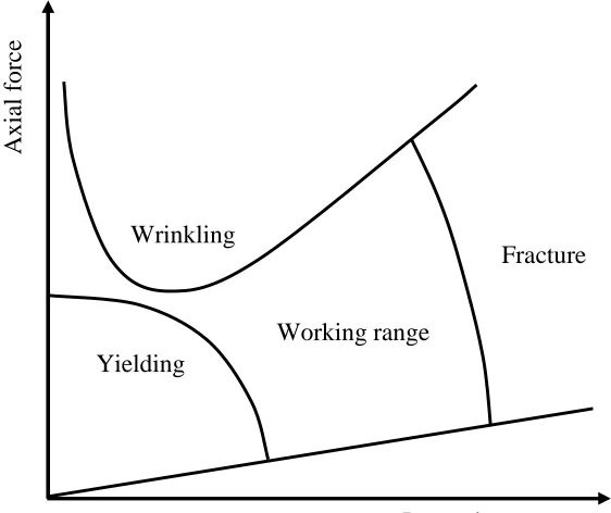
Asnafi (1999) identified process limits for wrinkling, fracture, yielding, and sealing, and sketched a THF process window where the safe working range is dependent on the combination of the axial compressive force and internal pressure (Fig. 1.1).

Chu and Xu (2004a, 2004b) formulated a theoretical process window for predicting forming limits induced by buckling, wrinkling, and bursting of free-expansion THF. An

Fig. 1.1 Example of THF process window (Adapted from Asnafi, 1999) Internal pressure Wrinkling

Fracture

Working range

A

x

ia

l

fo

rc

e

optimal loading path was also proposed in the process window diagram (PWD) with an attempt to define the ideal forming process. However, an assumption of a proportional loading path was adopted. Since using a piece-wise linear combination of strain paths might enable the process to achieve a larger expansion ratio for the THF process, such a curved loading path will result in translating the boundary of the process window. The path dependency of the PWD was not discussed in their paper. Moreover, the window for an industrial part may be very small due to multi-stage forming and is difficult to determine.

1.1.4 Multi-objective optimization

Engineering design, by its very nature, is non-linear and multi-objective, often requiring tradeoffs between disparate and conflicting objectives. For instance, for typical hydroformed components, there are competing objectives; there is a need to reduce the risk of necking/fracture and wrinkling, minimize thinning, while achieving a specified geometry and maintaining a reasonably uniform thickness distribution throughout the part. This constitutes a problem of multiple objectives.

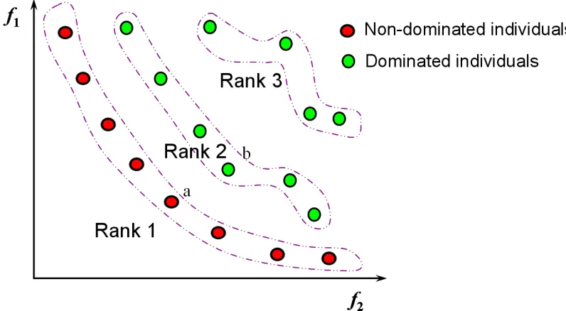
One way of defining optimality in a more precise way is via the concept of “dominated solutions”. A point or solution b for hydroforming problem (green dot) is called “dominated” by another point a (red dot) when all objective values of a are smaller (Deb et al., 2002) (Fig. 1.2). The set of non-dominated points is called the “Pareto front” or “Pareto solutions”, and represents a set of optimal solutions. It may be comparatively easier to choose among a given set of alternatives if appropriate decision support is available for the decision maker (DM). Hence, the main purpose of multi-objective problems is to find such non-dominated points.

Fig. 1.2: Pareto set for multi-objective optimization with two objectives (Minimizing)

Ingarao et al. (2009) pointed out that two main phases should be developed in metal forming optimization in order to reach an optimal solution: the modelling phase and the computation phase. In the modelling phase the proper design variables to be optimized must be selected, and a correct formulation of the objective function must also be developed. Moreover, in most metal forming optimization problems the analytical linkage between the design variables and the objective function is not available.

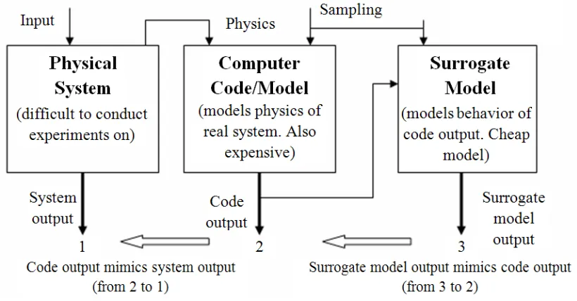
acceptable load path. The cost of the complete series of simulations, however may be expensive. To save computation time, a widely accepted practice is to build an inexpensive approximation model to replace the time-consuming simulation problem, and to optimize the surrogate model instead of the original finite element simulations.

Recently, the Kriging method, or design and analysis of computer experiments (DACE) (Sacks et al., 1989), which originated from the field of spatial statistics, has attracted attention in the area of metal forming (Stander et al., 2007; Lee and Kang, 2007). This model predicts the value of the unknown point using stochastic processes. Sample points are interpolated with the Gaussian random function to estimate the trend of the stochastic processes. However, the Kriging model is not a suitable method for data sets which have anomalous pits or spikes, or abrupt changes such as breaklines, and it is a much more complex method to use compared to the response surface methodology.

1.2

Problem statement

Currently, the development of THF processes is greatly delayed by long lead times, which result from many iterations of either trial-and-error based finite element (FE) simulations or expensive changes to prototype tooling. Moreover, the hydroformability of tubular parts is affected by a large number of parameters such as material properties, tube geometry, complex die-tube interface phenomena, and process parameters (i.e. loading paths). Consequently, more powerful design tools are needed to help engineers design better products and robust processes and to reduce lead time and cost. As a result, the goals of the proposed work are to:

1. Determine a forming severity indicator for hydroformed tubular parts and establish a general form of objective functions for THF;

2. Investigate two optimization strategies for solving multi-objective optimization problems: normal boundary intersection (NBI) and multi-objective genetic algorithm (MOGA);

experiments (e.g. central composite designs, Latin hypercubes) and surrogate approximations (e.g. response surfaces, Kriging models) is considered to rapidly explore and capture the Pareto frontier;

4. Investigate both piece-wise linear pressure and pulsating pressure paths;

5. Investigate applications in straight tube, pre-bent tube and industrial part hydroforming to validate the proposed algorithm.

1.3

Dissertation Organization

Finally, the outline of this dissertation work by chapters is: Chapter 1: Introduction and problem statement

Chapter 2: Literature review

Chapter 3: A hybrid forming severity indicator for tube hydroforming simulation

Chapter 4: Multi-objective optimization and sensitivity analysis for tube hydroforming using normal boundary intersection

Chapter 5: Loading path design using multi-objective genetic algorithm for a straight tube and an industrial part

Chapter 6: Optimization of loading path in hydroforming with pulsating pressure Chapter 7: Loading path design in multi-stage tube forming

Chapter 2: Literature Review

In this chapter, the background of this research will first be presented, then the literature on THF optimization will be reviewed. A review of the current optimization software development and their advantages and shortcomings will also be presented. Finally, a new level of metamodelling closely linked to the multi-objective optimization process is introduced.

2.1 Tube hydroforming

2.1.1 Introduction

Tube hydroforming (THF) uses a pressurized fluid and axial compressive forces to plastically deform a tube into a desired shape. A typical straight tube hydroforming process is shown in Fig. 2.1. For parts with a more complex geometry, the process may also include preparing the tube, preforming, hydroforming, trimming or end cutting.

As far as the author could survey, approximately one half of the technical papers written and published on various aspects of hydroforming address THF processes.

2.1.2 Examples of hydroforming in the automobile industry

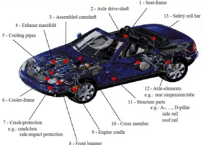
Some of the most common applications of tube hydroforming can be found in the automobile industry. In 2002, the American automobile maker, Chrysler, began incorporating hydroforming to help reduce chassis vibration on its redesigned Dodge Ram (http://www.thomasnet.com). Likewise, General Motors' (GM) suppliers began using hydroforming to create suspension parts. There was an eventual increase of approximately 20 percent in manufacturing productivity for GM, and the switch to hydroforming may have contributed to the gain. GM continues to use hydroforming in its production methods. In 2006, it became one of the first automakers to use this process to create structural products on vehicles (Pontiac, Chevrolet) for several of its brands. Other examples of hydroforming in the automobile industry include the making of engine cradles for various, Ford, and Chrysler models. The process has also been used by several European automobile manufacturers, such as Volkswagen, who switched from deep drawing to hydroforming in order to create unibody frames for some of their vehicles. In addition, parts such as roof pillars, frame rails, engine cradles, rear axles, and exhaust manifolds are widely manufactured using tube hydroforming techniques (Ahmetoglu and Altan, 2000; Dohmann and Hartl, 1997). Fig. 2.2 illustrates some typical hydroformed tubular parts in an automobile.

Fig. 2.2 Typical hydroformed parts in an automobile (Adapted from http://nsm.eng.ohio-state.edu/Advances_in_Hydro.swf)

2.2 Conventional design method of loading path

After the 1970's, a number of studies were carried out on different aspects of tube bulging, among these being the work of Hashmi (1981,1983), Hashmi and Crampton (1985), Dohmann and Klass (1987), Murata et al. (1989) and Thiruvarudchelvan and Lua (1991), which led to an understanding of tube bulging under axial compressive load. The compressive load, as found in these works, delays the onset of plastic instability by ''feeding'' extra material into the forming zone.

Rama et al. (2003) developed a two-dimensional numerical method based on membrane theory to explicitly relate the deformation sequence with the pressure loads for tube expansion. However, the loading parameters (i.e.pressure and end feed) are still largely determined by the experience of hydroforming press operators.

Prior to the introduction of an analytical method, some early experiments were performed to achieve better bulge forming. Limb et al. (1973) carried out bulge forming of tubes of different metals and alloys with different wall thicknesses. It was found that increasing the internal pressure incrementally in steps during the axial load application was the most satisfactory method of bulging thin walled tubes. Manabe et al. (1984) carried out experiments using a computer-controlled testing apparatus to examine the influence of linear and non-linear loading paths on the behavior of thin-walled aluminum tubes during hydroforming. Thiruvarudchelvan and Lua (1991) developed a device for applying an axial compressive force proportional to the internal pressure and obtained an optimum ratio for maximum bulging. Dohmann and Hartl (1994,1996) presented a flexible tool system that divided the die into segments that can be driven separately during the process. Bieling (1992) carried out a number of experiments of bulge forming with tubes and hollow shafts to investigate a range of suitable bulge forming parameters.

2.2.1 Analytical method

Bieling (1992) developed a group of equations to determine the suitable internal pressure and axial force for stepped cross-sectional tubes. Ahmed and Hashmi (1997) provided a theoretical method for bulge forming to estimate the internal pressure, axial load and clamping load which are required to design the dies, punches and accessories for the process.

forming limit curve (FLC) was used as an aid to finite-element simulations in component and process design. The study showed that the FLC of the tube material must be determined by bulge test. Kim and Kim (2002) used the analytical models to determine the forming limits for the THF process and demonstrated how the loading path and material parameters of the strain hardening exponent (n-value) and anisotropic parameter (r-value) influenced the forming results.

Rimkus et al. (2000), Jirathearanat et al. (2004) and Koç (2002, 2003) utilized simple analytical methods to obtain initial values of yielding, maximum pressure and axial feeding for the loading path design.

Fig. 2.3 Load-curve for internal pressure vs. time (Adapted from Rimkus et. al, 2000)

In Fig. 2.3, the internal pressures Pi1 (at point 1) and Pi2 (at point 2) were determined as

follows:

y

i

P

P

=

0

.

9

(2.1)

y

i

P

P

=

(

1

.

2

~

1

.

4

)

(2.2) where, Py is the pressure to yield the tubular part. However, the calibration pressure was

determined by the radius-pressure curve, and was affected by the tube wall thickness, the material and the radius which was to be achieved.

Jirathearanat et al. (2004) analytically estimated the initial group of process parameters for Y-shape THF, optimized it using FEA, and confirmed that higher material feeding at the initial stages of hydroforming was beneficial. Koç and Altan (2002) conducted determination of process limits and parameters for hydroforming by applying widely known plasticity, membrane and thin/thick walled tube theories, and analytical predictions were compared with their experimental findings. Koç (1999, 2002) estimated the yield pressure Py and bursting pressure Pb according to the following relationships

0 0 0

2

t

D

t

P

−

=

σ

P_{b UTS}

− =

σ

(2.4) where σ_yis the yield stress,

σ

the initial wall thickness and D is the initial outer diameter. An estimation of the 0

maximum calibration pressure Pc at the moment of die corner filling was obtained based

upon an estimation of the pressure required to achieve a certain target corner radius (R_C), according to the following equation (Koç and Altan, 2002):

      − = t R R P C C UTS c ln 3 2 _σ (2.5)

where σUTSis the ultimate tensile stress of the material and t is the current wall thickness. Eq. (2.5) indicates that the pressure required to achieve a certain corner radius increases as the radius decreases.

Braeutigam and Butsch (1992) proposed an empirical equation that is suitable as a first approximation of the maximum internal pressure required to hydroform a part:

C UTS k

R t P ≈1.2

σ

(2.6)

Guan et al. (2006, 2008) used Fourier series based finite element analysis to study the axisymmetric bulge of tubes. Four to six Fourier series terms to approximate displacement were used to quickly and efficiently model the cross-section of the tube and accurately predict the final deformed shape and strain distribution.

All these analytical models provide an estimation of the internal pressure at some key stages during the forming process. Moreover, these models have mostly been limited to the axisymmetric bulging of tubes, and as such, are useful during the early stages of the process design. However, due to the highly non-linear nature of the process, theoretical studies to date have produced a relatively limited understanding of the mechanics of the hydroforming process.

2.2.2 Finite Element Method

Undoubtedly, almost all tests of the THF process were conducted experimentally and involved significant costs and time. The computer simulation of THF processes using the finite element method (FEM) has proven to be efficient and useful (Ponthot and Kleinermann, 2006), as it allows for the virtual testing and comparison of several candidate processes, thus avoiding the use of costly “trial and error” prototype tests. Several tools based on FEA simulations and experiments were developed to determine the process window for failure-free hydroforming (Gao et al., 2002; Manabe and Amino, 2002; Strano et al., 2004).

Palumbo et al. (2004) performed experiments and numerical simulations of the forming of a compound part consisting of a cylindrical region (the base) and a square part (the protrusion). Hwang et al. (2002) proposed a mathematical model and a finite element code ‘‘DEFORM’’ to examine the relationship between the internal pressure and the bulge height of the tube during the bulge hydroforming process in an open die. The effects of various forming parameters, such as the die entry radius, the initial thickness, the initial length of the tube, etc., upon the forming pressures were discussed. Lei et al. (2001) developed a three-dimensional rigid-plastic finite element model, HydroForm-3D, to analyze several typical hydroforming processes such as tee extrusion, cross-extrusion, the hydroforming process combined with the pre-bent process and subframe. The hydraulic pressure force was applied to the normal direction of the tube workpiece by integrating the pressure with respect to each element’s surface area. MacDonald and Hashmi (2000) performed a finite element simulation of the manufacture of cross branches from straight tubes to investigate the effects of varying process parameters. It was concluded that when designing processes to bulge form cross-joints that compressive axial loading should be used in combination with pressure loading where possible; friction should be kept to a minimum where maximum branch height is required and greater tube thickness should be used when seeking to reduce stress and thinning behaviour in the formed component. Yoon et al. (2006) extended the direct design method that was based on ideal forming theory for the design of non-flat preform for THF processes. A preform optimization methodology for non-flat blank solutions was proposed based on the penalty constraint method for the cross sectional shape and length of a tube. The hybrid membrane/shell method was employed to the capture thickness effect while maintaining membrane formulation in the ideal forming theory.

Advantages and disadvantages

is required that will minimize numerical simulation time, while maintaining a high level of accuracy.

2.3 Optimization method in tube hydroforming

The finite element analysis is able to provide a valuable understanding of the hydroforming process. Nevertheless, the trial-and-error approach to optimizing the process design can be very time consuming. Instead, this iterative FEA method can be performed systematically and automatically in conjunction with various optimization methods, and the determination of the loading path can be treated as a classical optimization problem. Once the optimal loading path is found it can be utilized to maximize the part formability.

There are a variety of optimization strategies which can be classified into two categories: gradient and non-gradient methods (derivative free optimization). Gradient-based methods include the steepest descent method, the Newton, and the Quasi-Newton method used for linear and non-linear static optimization problems. For highly complex problems (optimizing a very large number of design variables), non-gradient-based methods are normally applied, such as response surface methods and genetic algorithms. However, the methods can also be classified in terms of computational intelligence (Engelbrecht, 2007): classical optimization (gradient-based and some of the non-gradient-based methods) and intelligent optimization (e.g. artificial neural networks (ANN), evolutionary computation (EC), swarm intelligence (SI), artificial immune systems (AIS), and fuzzy systems (FS)).

2.3.1 Classical optimization algorithms

2.3.1.1 Conjugate Gradient Method

with the finite element method, have been developed and applied to structural engineering and to the area of metal forming.

Yang et al. (2001) sought to determine the optimal hydroforming process design using numerical simulation combined with an optimization tool that is based on the gradient method and sequential quadratic programming. A B-spline curve with six control points was used to describe the load path. The tube thickness variation was minimized. In addition, the thickness sensitivity analysis with respect to initial pressure was carried out. Fann and Hsiao (2003) applied the conjugate gradient method with the FE method to investigate how various loading conditions affect the thickness distribution in the tube wall and the part geometry. They also sought to determine an optimal loading condition using both a batch mode and a sequential mode, where the batch mode defined in their study was used to optimize all the process variables at once in view of their influence on the final result. The sequential mode was used to optimize the loading conditions one stage at a time in view of their effect on the results at each intermediate forming stage. The sequential mode generated a loading path with better tube quality than that generated with batch mode.

Lorenzo et al. (2006) proposed an integrated approach which combines FEM simulations and gradient-based optimization techniques with the aim to determine the optimum blank contour in a typical 3-D deep drawing operation. An optimal blank shape was obtained which guarantees that thinning is minimized.

Advantages and disadvantages

Since the operation is gradient-based, there are two situations in engineering where applying the finite-difference derivative approximation is inappropriate: when the function evaluations are costly and when they are noisy. In the first case, it may be prohibitive to perform the necessary number of function evaluations (normally no less than the number of variables plus one) to provide a single gradient estimation. In the second case, the gradient estimation may be completely useless. Moreover, in some complex problems, either the derivatives are unobtainable, or the finite differences approximation is expensive. Furthermore, considering the optimization method (Conjugate Gradient Method – constrained or non-constrained conditions), it is simple to carry out, but needs a good initial point and the penalty scalar for the step adjustment. Consequently, it is difficult to fulfill the multi-objective optimization using the conjugate gradient method.

2.3.1.2 Self-feeding and adaptive simulation method

Aue-U-Lan et al. (2004) proposed to use self-feeding (SF) and adaptive simulation (AS) to find robust and cost effective techniques to determine optimal loading paths. The implementation of these two approaches is now presented.

(1) SF approach

This method was designed to restrict the search for the loading path to a proper family of curves and to select the optimum within this family. This method contains two steps: 1) Determine the relationship between internal pressure (P) and axial feed (dax), where the process is simulated by imposing only the internal pressure versus time. The friction at the interface is assumed to be zero.

axial feed is increased by a certain amount using a scaling factor, α (α*SF), as shown in Fig. 2.4. This scaling factor was varied until a successful part is formed.

Fig. 2.4 SF loading paths: α is a scale factor to increase the amount of axial feeding (Adapted from Aue-U-Lan et al., 2004)

(2) AS approach

Fig. 2.5 Schematic procedure of the AS ( Pi: internal pressure, ∆Pi: internal pressure

increment, Piy: yield pressure, ∆Da: axial feed increment). (Adapted from Aue-U-Lan et al., 2004)

The SF is a “systematic trial-and-error” approach for establishing a family of loading paths via FEA. The THF experiments done using this approach have shown that SF can significantly reduce the number of trial runs necessary for process development. However, these two methods sometimes failed to find an optimal solution.

2.3.2 Intelligent optimization algorithms

2.3.2.1 Fuzzy adaptive method

Though it is possible to determine suitable process parameters by repeating a series of FE simulations, this trial-and-error process can be extremely time-consuming. In order to reduce the time for optimization, some researchers combined the fuzzy method with FE simulation to identify the optimal loading path. Adaptive simulation uses different judgment rules in order to improve the results of the simulation: when defects or quality conditions are detected the loading path is automatically adjusted.

processor, sensor and actuator in a real closed-loop system. Process control can be accomplished by using the current feed-back to modify the control parameters for next step of analysis. The control values are determined automatically based on artificial intelligence (AI) rules in the user-defined subroutine. The simulated results of the next step may include the effect of the process-controlled path.

Wu (2003) investigated the adaptive simulation of T-shape tube hydroforming by combining the FE code LS-DYNA with a fuzzy logic controller subroutine. During the simulation process (Fig. 2.6), subroutines can adjust the loading path according to the values of the minimum tube thickness and its variance. The goal of a better thickness distribution at the side branch of the formed part was achieved. Comparing with other linear loading paths, this adaptive control method led to better results.

Fig. 2.6 The process of the adaptive simulation (Adapted from Wu, 2003)

Strano et al. (2004) investigated both a self-feeding simulation approach and an adaptive simulation approach to determine successful loading paths in a timely manner. Strano et

al. (2001) proposed a defect criterion based on the geometry to detect the wrinkling

T-branch forming with a counterpunch with a validation of an aluminum alloy THF. An adequate loading path was searched using the fuzzy control algorithm, and the quality of the hydroformed product was improved compared to parts that were formed with a loading path determined on the basis of experience. Ray et al. (2004) determined the optimal load paths for X- and T-shaped hydroformed parts using FE simulations and an intelligent fuzzy logic-based load control algorithm: this enabled them to maximize part expansion while simultaneously maintaining wall thickness, forming stresses and plastic strains within the allowable limits. Aydemir et al. (2005) presented an adaptive method using a fuzzy knowledge-based controller to obtain a more efficient process control for THF processes, and therefore avoiding the onset of wrinkling and bursting with the help of dedicated stability criteria. The wrinkling criterion uses an energy-based indicator inspired by the plastic bifurcation theory. For necking followed by bursting, a criterion based on the forming limit curve was employed. Park et al. (2005) analyzed the empirical relationships between process parameters and hydroformability by fuzzy rules. Many process parameters were converted to a quantitative relationship by the use of approximate reasoning of a fuzzy expert system. Finally, Lorenzo et al. (2004a, 2004b) proposed a fuzzy system integrated with a FE code to obtain a closed-loop control for process design.

Advantages and disadvantages

The fuzzy adaptive method may well reduce the amount of simulation. Compared to optimization methods the fuzzy method required less simulation time and is easier to implement. However, the accuracy of this method depended on the selection of fuzzy rules and the member function.

2.3.2.2 Genetic algorithms

improved pressure profile and feed rate can be identified based on intuition and experience. Although adaptive simulation and fuzzy control can be used to find an appropriate loading path, it may not lead to an optimal solution within a reasonable time. There is a need, therefore, to develop an improved methodology to determine the loading paths.

Abedrabbo et al. (2005, 2009) presented a method using a Genetic Algorithm (GA) search method in combination with LS-DYNA to optimize the process parameters to determine the best loading paths of THF in a square-shaped die. Their goal was to maximize formability by identifying the optimal internal hydraulic pressure and feed rate while ensuring that the strains in the part did not exceed the forming limit curve (FLC). The hierarchical evolutionary engineering design system (HEEDS) was used in combination with the nonlinear finite element code LS-DYNA. Compared to the best results of a manual optimization procedure, a 55% increase in expansion was achieved by the automated procedure.

Roy et al. (1997) described an adaptive micro-genetic algorithm (µ GA) for design optimization of process variables in multi-stage metal forming processes (e.g. multi-pass cold wire drawing, multi-pass cold drawing of a tubular profile and cold forging of an automotive bar).

Advantages and disadvantages

are only rare applications of this approach to THF, further improvements are needed, such as the optimization of multiple objectives.

2.3.3 Summary of the classical and intelligent method

While classical optimization (CO) algorithms have been shown to be very successful (and more efficient than intelligent algorithms like GAs) in linear, quadratic, strongly convex, unimodal and other specialized problems, GAs have been shown to be more efficient for discontinuous, non-differentiable, multimodal and noisy problems. GA and CO differ mainly in the search process and the information about the search space that is used to guide the search process:

• The search process: CO uses deterministic rules to move from one point in the search space to the next point. GA, on the other hand, uses probabilistic transition rules (Engelbrecht, 2007). Also, GA applies a parallel search of the search space, while CO uses a sequential search. A GA search starts from a diverse set of initial points, which allows for a parallel search of a large area of the search space. CO starts from one point, successively adjusting this point to move toward the optimum.

• Search surface information: CO uses derivative information, usually first order or second-order, of the search space to guide the path to the optimum. GA, on the other hand, uses no derivative information. The fitness value (i.e. the objective value) of individual candidate solutions is used to guide the search.

2.3.4 Multi-objective optimization

Recently, multi-objective optimization algorithms have been increasingly applied to metal forming processes in which several objectives must be achieved simultaneously. Hereinafter, some concepts related to this algorithm are briefly discussed.

2.3.4.1 Multi-objective optimization problem (MOP)

Minimize: F(x)=[F1(x),F2(x),...,Fm(x)]T subject to:

U L

x x x

x g

x h

≤ ≤

≤ =

0 ) (

0 ) (

(2.7)

where F is the vector of objective functions, x ∈ Rn _{is the vector of decision variables, h}

and g are the possible sets of equality and inequality constraints, respectively, and _{x and} L U

x are the lower and upper bounds for the decision variables. Finally, n is the number

of variables and m is the number of objectives.

2.3.4.2 Pareto optimality

Pareto optimality is defined using the concept of domination (Zitzler and Thiele, 1999). Given two parameter vectors a and b, a dominates b if and only if (iff) a is at least as good as b in all objectives, and better in at least one. Similarly, a is equivalent to b iff a and b are identical to one another in all objectives. A parameter vector a is Pareto

optimal iff a is non-dominated with respect to the set of all allowed parameter vectors.

Pareto optimal vectors are characterized by the fact that improvement in any one objective means worsening at least one other objective.

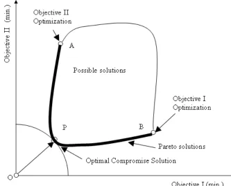
The Pareto optimal set is the set of all Pareto optimal parameter vectors, and the

corresponding set of objective vectors is the Pareto optimal front. Fig. 2.7 shows the

Pareto front for two objectives. The Pareto optimal set is a subset of the search space, whereas the Pareto optimal front is a subset of the solution space.

Mathematically, a feasible solution x* is a Pareto-optimal (or dominated, or non-inferior, or efficient) solution if there exists no x such thatF_i(x)≤F_i(x*) for all i=1, ..., n with Fj(x)<Fj(x*) for at least one j=1,...,m. This definition signifies that all non-dominated solutions are optimal in the sense that it is not possible to improve one objective without degrading one or more of the other ones. After obtaining the set of Pareto-optimal solutions, the designer is able to select a suitable compromise between all objectives. In order to help the decision-making process, it is important to find a set of solutions as diverse as possible and uniformly distributed along the Pareto front.

For Pareto optimality (Fig. 2.7), there are several methods available to determine the Pareto set (weak or strong), such as the weighted sum method, the ε-constraint method, the goal attainment method and the multi-objective GA method. In this work, the Normal

Fig. 2.7 Pareto-optimal solution for two objectives

2.3.4.3 Surrogate model

A surrogate model, or meta-model, is constructed to replace the time-consuming FE simulation, and will be used together with the multi-objective optimization algorithms to find the optimal loading path parameters in hydroforming applications. Fig. 2.8 shows the entire philosophy of surrogate modelling in the form of a flow chart.

More details of this method can be found in section 2.3.5.

Fig. 2.8 Surrogate modelling philosophy (Adapted from Kulkarni, 2006)

2.3.4.4 Taguchi method

The S/N ratio for the lower-the-better characteristics related to the tube hydroforming is given by

   

 

∑

− =

= n i i

y n N

S

1 2

1 log 10

/ (2.8)

where yi indicates the measured objectives, and n is the number of simulation repetitions

under the same design parameter conditions. Regardless of the definition of the S/N, a greater S/N ratio always corresponds to a better quality characteristic.

In the Taguchi method, a statistical method of analysis of variance (ANOVA) is further employed to quantitatively investigate the effects of the parameters on objectives. A design parameter is considered to be significant if its influence is large compared to the virtual experimental error.

2.3.4.5 NBI

The NBI method is a preferred approach for multi-objective optimization and was developed by Das and Dennis (1998). The details of this method are provided in Chapter 4.

2.3.4.6 Multiobjective evolutionary algorithm (MOEA)

Since the first studies on evolutionary algorithms (EA), major research and application of EAs in multi-objective optimization, only started in the early of 1990s. However, the effectiveness of evolutionary computation methodologies in the solution of multi-objective optimization problems has generated significant research interest in recent years.

Some basic terminology is given to aid in the understanding of the subsequent work. 1. Parent: a solution used during crossover operation to create a child solution.

2. Children (or Offspring): new solutions (or decision variable vectors) created by a combined effect of crossover and mutation operators.

4. Fitness: a fitness or a fitness landscape is a function derived from objective function(s), constraint(s) and other problem descriptions which is used in the selection (or reproduction) operator of an EA.

5. Crossover: an operator in which two or more parent solutions (chromosome 1 and 2, Fig. 2.9a) are used to create (through recombination) one or more offspring solutions. The operation is illustrated by swapping two parts at the crossover point in Fig. 2.9a. 6. Mutation: an EA operator which is applied to a single solution to create a new perturbed solution (Fig. 2.9b). A fundamental difference with a crossover operator is that mutation is applied to a single solution, whereas crossover is applied to more than one solution.

(a) Crossover (b) Mutation

Fig. 2.9 The crossover and mutation operations in EA

The NSGA-II algorithm developed by Deb et al. (2002) has been a popular optimization tool in recent years. It adopts an elitism strategy and crowding-distance calculation, which offer a much better spread of solutions and better convergence in most problems near the true Pareto-optimal front compared to Pareto-archived evolution strategy and strength-Pareto Evolutionary Algorithm – two other elitist multi-objective evolutionary algorithms (MOEA) that pay special attention to creating a diverse Pareto-optimal front. The algorithm of NSGA-II and its improvements will be detailed in chapter 5.

Fig. 2.10 Schematic of a two-step multiobjective optimization procedure (Adapted from

2.3.5 Meta-model based multi-objective optimization

By properly constructing meta-models, designers can address the challenge posed by prohibitively high computational times. The resulting approximation is computationally efficient functions and allows for a comprehensive exploration of the design space, and may yield significantly improved designs. The literature review also shows the trend in THF: from single-objective optimization to multi-objective optimization; from direct FE simulation to meta-model based optimization.

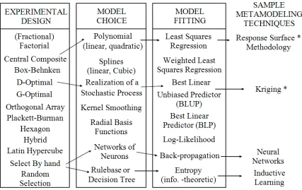
In order to accelerate the calculations, a variety of surrogate methods are used to substitute the FEA simulations: Polynomial regression (Myers and Montgomery, 2002), Radial basis functions (Hussain et al., 2002), ANN (Rafiq, 2001) and Kriging models (Strano, 2006). It is obvious that the allocation of the sampling points used to build the approximation have an effect on the final performance of the surrogate model. Many schemes and criteria have been proposed to allocate a-priori the sample points in a convex domain of interest: Factorial design, Box-Behnken, Koshal, Central Composite design, D-Optimal and Space-filling design. All these efforts are made to approach the true response surface of the practical problems. It is practically difficult to conclude which one is most suitable for allocation and reduction of sampling points to reach a desired precision.

There are normally three stages that describe this methodology: 1) First stage: design of experiments (DOE).

2) Second stage: selection and construction of a surrogate model. 3) Third stage: multi-objective optimization.

2.3.5.1 Design of experiments