A beta-gamma angular correlation experiment using arsenic-74.

Scholarship at UWindsor

Scholarship at UWindsor

Electronic Theses and Dissertations Theses, Dissertations, and Major Papers

1-1-1965

A beta-gamma angular correlation experiment using arsenic-74.

A beta-gamma angular correlation experiment using arsenic-74.

Winston Armstrong University of Windsor

Follow this and additional works at: https://scholar.uwindsor.ca/etd

Recommended Citation Recommended Citation

Armstrong, Winston, "A beta-gamma angular correlation experiment using arsenic-74." (1965). Electronic Theses and Dissertations. 6373.

https://scholar.uwindsor.ca/etd/6373

A

p > - X

BY

WINSTON ARMSTRONG

A Thesis

Submitted to the Faculty of Graduate Studies through the Department of Physics in Partial Fulfillment

of the Requirements for the Degree of Plaster of Science

at The University of Windsor

Windsor, Ontario

INFORMATION TO USERS

The quality of this reproduction is dependent upon the quality of the copy

submitted. Broken or indistinct print, colored or poor quality illustrations and

photographs, print bleed-through, substandard margins, and improper

alignment can adversely affect reproduction.

In the unlikely event that the author did not send a complete manuscript

and there are missing pages, these will be noted. Also, if unauthorized

copyright material had to be removed, a note will indicate the deletion.

®

UMI

Copyright 2008 by ProQuest LLC.

All rights reserved. This microform edition is protected against

unauthorized copying under Title 17, United States Code.

ProQuest LLC 789 E. Eisenhower Parkway

E. E. Habib

H. Ogata

^

A. van Wijgaarden

In this thesis, the theory of beta-gamma angular cor­

relation is discussed briefly. Beta decay is analysed inoluding

allowed and first forbidden beta decay as well as a method of

analysing data from the Ag coefficient to determine whioh nuclear

model is applicable. The corrections applied to the experimental

measurements are introduced. An experiment is performed whioh

measures the beta-gamma angular correlation coefficient, Ag, for

the cascade

2~(

2~{ {3~)2+(

NEGATRONS

w

A2

1 .6 0 .0 1 2

-

1 .8

_-0.045

-

2 .0

POSITRONS

-0.044

-

1 .8

_{0.015 i}

2 .0

0.019 £

2 .1 0.0 3 0

i

2 .2

0.025 £

The positron data is used to examine the structure of the

first excited level in G e ^ . The negatron data was not used due to

insufficient precision or not enough points. Both the shell model

and the collective model can be made to fit the positron data. The

2

satisfactory shell model configurations found are (f^yg) ^

9

2

(f^/g) (

89

2

U

tinguish between the above configurations and a rotational excit­

ation, more data, such as the shape factor and the beta-circularly

polarized-gamma directional correlation coefficient, is required.

I wish to express my sincere thanks to Dr. E.E. Habibj

without whose guidanoe and counsel this experiment could not have

been carried out.

My thanks go to Dr. Ogata who performed the calculations

to determine which nuclear model was applicable. I would like to

express my gratitude to Mrs. Robert Armstrong for typing the

manuscript.

PAGE

TITLE PAGE i

ABSTRACT iii

ACKNOWLEDGEMENTS iv

TABLE OP CONTENTS V

LIST OP TABLES vi

LIST OP ILLUSTRATIONS vii

CHAPTER I THEORY 1

1. Angular Correlations 1

2. Beta Decay Theory ₃

(ii) First Forbidden Beta Decay 7

(iii) ^ Approximation 10

(iv) Modified B . . Approximation

X J 15

(v) Method of Using the Experimental Data

to Distinguish Between Two Models

16

CHAPTER II As74 EXPERIMENT 19

1. Apparatus 20

2. Source Preparation 23

3. Preliminary Adjustments 23

(i) Centering of the Source 23

(ii) Centering of the Gamma Probe 23

4. Experimental Procedure ₂₅

5. Treatment of the Data

26

CHAPTER III INTERPRETATION OP RESULTS AND CONCLUSIONS 36

1. The Shell Model 36

2. Analysis of Data 38

3. Conclusions 42

BIBLIOGRAPHY

(v)

TABLE # NAME OF TABLE PAGE

I Fermi and Gamow-Teller Interactions 5

II Summary of Allowed and First Forbidden Matrix 6

Elements

III Asymmetry, Ag Coefficients and Solid Angle 30

Corrections for Negatrons

IV Asymmetry, Ag Coefficients and Solid Angle 31

Corrections for Positrons

V Corrections for Chance and Scattering Positrons 32

and Negatrons

VI Table of Coincidences to Get a(w) - Positrons 33

VII Table of Coincidences to Get a(w) - Negatrons 35

VIII Table of the Shell Model 37

IX V and Y Corresponding to the Intersects of the 41

Theoretical Circles with the Meniscus

X Calculated Centres of Circles and Radii 41

(Matumoto's Method)

FIGURE # TITLE PAGE

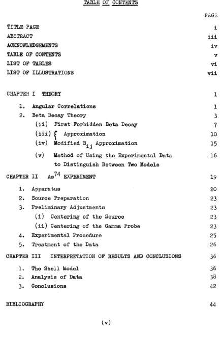
1.1 2 (^3) 2+ ( K ) 0+ Cascade 17

2.1 A s ^ Decay Scheme

19

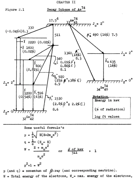
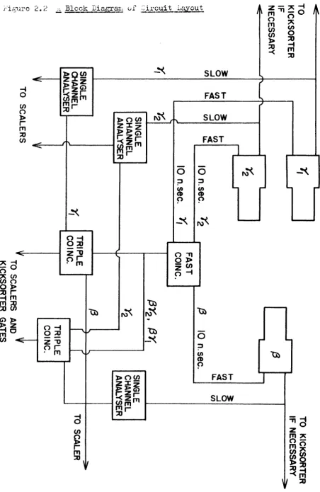
2.2 A Block Diagram of Circuit Layout 21

2.3 A Two Fold Fast Coincidence Circuit 22

2.4 The Gamma Singles Spectra 24

2.5 The Gamma 1 Spectra in Coincidence with the 27

Betas

2.6 The Gamma 2 Spectra in Coincidence with the 28

Betas

2.7

i>

§

2.8

i

i

3.1 Plot of V vs. Y 40

THEORY

1. Angular Correlations

The probability of emission of a particle or quantum by a

radioactive nucleus depends in general on the angle between the

nuclear spin axis and the direction of emission. Under ordinary

circumstances the total radiation and the radiation for an individual

fi

transition 1^*— ♦Ig from a radioactive sample is isotropic because

the nuclei are randomly oriented in spaoe.

However, in a two step cascade transition, such as

where R denotes the type of radiation,

eg-(^»

$

are emitted from the same nucleus.

The existence of an angular correlation arises because

the direction of the first radiation is related to the orientation

of the angular momentum, I„ , of the intermediate level. This

orientation can be expressed in terms of the

magnetic-angular-momentum quantum number, mg, with respect to the direction of the

first radiation. If Ig is not zero, and if the lifetime of the

intermediate level is short enough so that the orientation of Ig

persists, then the direction of emission of the second radiation

will be related to the direction of Ig and hence to the first

radiation.

Many of the details of the complicated theory of these

angular correlations have been worked out. Experimental and

theoretical developments have been summarized in a number of

Qlto.s

excellent review articles. (bLA'i'T.

52

53

51

For the generalized R,-R„ cascade 1^(1,)lB (l„)lc the

angular-correlation function W(<P) for the angle

<p

50

i=L

l.a— W ( < ? ) d a = 2- A 9 .P0 .(cos f ) d A i=0

d

where A^^ are coefficients which aepend on l,and 1„, the orbital

angular momentum transferred by R, and R„ respectively.

L is the a M i a a l angular-momentum quantum number.

P g ^ C O S are the even Legendre Polynomials.

There are rigorous restrictions on the number of terms

in eqns. l.a; the highest even power of cos

<Q

21, or 2IB , or 21„ and will be one unit less than the smallest if

the smallest is odd. For example, if or ■§■, W(<^)=1, and the

angular correlation distribution will be isotropic.

A convenient experimental quantity is the

Anisotropy=A= -1 .

The conditions of validity of eqn. l.a must include all the

assumptions made in its derivation (for these consult EVANS.55)*

The information that can be obtained from angular

correlation work depends on the type of radiation observed («K,^,'5,e )

and on the properties that are singled out by the experiment

(direction, polarization, energy), and on the extranuolear fields

acting on the nucleus. Here we assume that the decaying nuclei

ntjh We.

are free, ie., that'

5

o<~^ and dirccti- nrl correlation information about the

obtained. The relative parities can be determined, however,

if one observes in addition to the direction also the polarization

of the gamma-rays, or if one measures the directional correlation

between conversion electrons^-"). The directional correlation of

a beta-gamma cascade depends not only on the nuclear spins and

parities, but also on the matrix elements involved in the

beta-transition.

In the first transition of a beta-gamma cascade, an

electron and a neutrino are emitted simultaneously. Formally,

this event is described by treating the process as if a neutrino

(antineutrino) enters the nucleus and a negatron (positron) is

emitted. In a beta-gamma correlation experiment one measures the

direction of the electron while the neutrino escapes unobserved.

The theoretical calculation of the angular correlation thus

necessitates an averaging over all neutrino directions and over

the spins of the neutrino and the electron. In our case for a

first forbidden beta-transition the expression for the beta-gamma

directional correlation is (MAT. 63). >*r* : t « 1

l.b— N(W,^) - l+A

2

2

2

2. Beta Decay Theory

In "Beta Decay" three processes can take place,

1

1

— ■>

V

1.3

1/

In 1.1, a neutron changes into a proton plus an anti­

neutrino and a negatron? in

1

2

negatron to form a neutron and a neutrino. 1.1 is called "Negatron

Emission", 1.2 is called "Positron Einission", and 1.3 is called

"Eleotron Capture".

The leptons (electron and neutrino) may be emitted with

spins parallel or anti-parallel. In the first case, the net spin

$

1

0

with respect to the neucleus. The case where the orbital angular

momentum,! , is zero, is called the allowed beta decay, L - 2,***,

1st forbidden,

2

J, of the leptons must obey the conservation of angular momentum

i.e. J = L + S, { If - 1 ^ < J < | l f + i j — 1.4

where

1

1

transition states.

If

S'

0

_ q J then J « 0 A I ■ 0 — 1.5

Also if

0

S

I

L - 0

j

then J “ 1

A I » 0, i 1

In these cases since L =

0

is not changed. The condition 1.5 is called the "Fermi Interaction"

and 1.6 the "Gamow-Teller Interaction". Thus we have pure Fermi

radiation ( A l = 0, 0 — > 0 transition) as well as pure Gamow-Teller

radiation (I— > 1 — l). Th© Allowed A l » 0, 1^ = 1^ ^ 0 consists

of both Fermi and Gamow-Teller radiation in proportions depending

on the relative ease with which the requisite final nuclear states

can be formed by the Ferjpi or Gamow-Teller couplings respectively.

TABLE # I

Fermi and Gamow-Teller Interactions

Order Of

Forbiddeness

Fermi

F

Gamow-Teller

G.T.

L *» 0 A I -

0

A i - o, ± i, o V o

L = 1

A t

o, i 1

A l

0

-

1, i 2

o

4

-o

no

0

?0

1<~^0

Fermi Theory

The Fermi theory has been very successful in describing

beta decay. Fermi constructed his theory on the model of the theory

of electromagnetic radiation. Fermi assumed that the nucleons

generate beta radiation in proportion to the current associated with

the neutron to proton transformation or its reverse.

Where W » ) describes a proton (neutron) if one agrees

to treat as identical the neutron and proton co-ordinates of the

transforming nucleon, then from the requirements of relativistic

invariance we get the coupling energy density

h ' g(Yp

h

Yn)

(fe X.

W *

c.c. is the complex conjugate.

g is Fermi's fundamental coupling constant and is respon­

sible f or the m a g n i t u d e of t he interaction.

Covariant densities other than the four-vector current can be

constructed within the Dirac description of the "internal state" of

tensor (T), an axial vector (A), and a pseudoscalar (P), besides

the four vector (V) used by Fermi. There was not a priori reason

for not expecting beta radiation to be generated by any of these.

However from experimental and theoretioal investigations, the form

of the nuclear beta-decay interaction is well-established. We know

that beta-decay violates parity completely and can be written V-A

(vector-axial vector) for electron (negatron) emission (reference

REV. M. 59)* Parity conservation is equivalent to saying that a

system is invariant under reflections; just as conservation of

total angular momentum, around any axis requires invariance under

rotations. The parity of a state of a nucleus is fixed but the

parity of the leptons during transitions from one state of fixed

parity to another is random.

TABLE II

Summary of Allowed and First Forbidden Matrix Elements

Matrix Element >v A J

£>rr

GT

L

Allowed Cv $

1

0

0, i 1 1

(no

0

0

+1 GT 0

First C. f Y

Forbidden

1 2

CA j ( P r / i ) } •

0

° v / rl

°T i 0 1

+

j

—> _{-1 +1}

CA J « * r )

J

0

0

_}

(no

0

0

-1

+1

Allowed and first forbidden nuclear elements and their

when regarded as a tensor.)

( A J is the change in angular momentum or nuclear

spin.)

( ATT is the change in parity.)

( L is the orbital angular momentum.)

2.(ii) First Forbidden Beta-Decav (WEID.

6

From Konopinski, the interaction density, , for the

beta decay interaction is given by

H/>

' f

J [ % *

% ]

dZ

where Y i and lj/g are the initial and final wave fens.

Cy and C^ are the vector and axial-vector coupling constants

with values C^. ■ (

1.415

0

004

10

^

°A +

~7T~ m

The index i refers to the nucleons building up the initial

and final wave fens. 7j>' q and l ^ a r e the wave fans for electron and

neutrino, respectively.

We can compare this interaction for beta decay with the

interaction of an electromagnetic current (r) with the electro­

magnetic field given by its vector potential A

^

J

Z

The similarity is noted when the beta decay interaction

is put in the form.

X l ffi/t(r)L/a.(r)d'C

which is the "lepton current", a four vector, dependent on a space

co-ordinate r. Iy*(r) also depends on the magnetic quantum numbers

of electron and neutrino. This "lepton current" interacts with the

"baryon current"

B/W.(r) =

^5

In each case two four-veotors have a point interaction. Consider­

ing first the approximations made in the simpler case of ^ radia­

tion. Here, the usual procedure consists in a multipole expansion

of the vector potential of the radiation field which is suggested

by the fact that the nuclear levels can be characterized by their

total spin J. This is justified because a multipole of order L has

a factor ( k r i n the expansion, where

k

current, that is, by the nuclear radius E.

Keeping the lowest order terms amounts to keeping two

types of matrix elements, e.g., the Ml- and E2- matrix elements in

the simplest case. Ml- is of order v/o in the nuoleon velocities

compared to the leading electric dipole term, E2- is of order kB

compared to the leading term. In many transitions v/o and kR are

of the same order of magnitude and therefore, in many nuclei

Ml-and E2- transitions have comparable widths.

In nuclear -decay, we have the same situation, except

for two faots,

Lyu

increases the number of pertinent nuclear matrix elements.

is a divergenceless quantity with a gauge-invariant

interaction. This has the consequenoe that there are no electro­

transitions corresponding to the electric monopole case are called

allowed transitions in/# -decay.

The first nonvanishing term in the multipole expansion of

■V* is the dipole term. It has a matrix element which we can

hriefly denote by £ r and it is (neglecting retardation) of order

kB and obeys the seleotion rule A j = 0 , - 1 (no 0 — >0), A T T = -1.

The corresponding terms in the expansion of L/x lead to the matrix

elements for first-forbidden

/Q

The interaction has been found to be one of Vector-Axial

Vector. The vector interaction oonsists of two parts,

oc

sition. The former is of order v/c in the nuclear co-ordinates, and

has the selection rule A j =

0

1

0

0

1

therefore, a first forbidden term. By keeping terms of order qr

and kr in the lepton currents where k and q are electron and

neutrino momentum respectively, the matrix element with the operator

1

J

originating from the vector interaction,

Joe

Correspondingly, the axial vector interaction consists of

two parts, tf*and The first term gives rise to an allowed matrix

element if one replaces the lepton current by one. If one again

keeps terms of the order qr and kr in the lepton current, this

interaction gives rise to the following three first-forbidden matrix

elements:

j C

r,

J

IjfkrJ . /“ I - J" [ IT,

+ *i (Tj - f

^ ^ € r j j

This is a convenient form because the trace is already contained

in r. The matrix ^ ^ is already of first—forbidden type,

being of order v/o.

The selection rules obeyed by the axial vector

first-forbidden nuclear matrix elements are obvious:

They all have A T T a -l, and

^

0

(no 0 — >0), and Bij has A j »

0

1

-

j

j

may be replaced by their values for r- > 0 . This does not hold for

expressions involving the other four matrix elements, where the

next term in the expansion of either the electron or the neutrino

wave functions has to be taken.

2.(iii) ^ Approximation

In the

^

« Z \ S W

E °

where Wq is the maximum total energy of t h e ^ particles, and has

its name from the fact that,

<*• Z c 2R = ) ’

OC is the fine structure constant,

Z is the nuclear charge,

E is the nuclear radius.

1.7a Coulomb forces in the wave fen. of the electron,"^, are much more

important than the next term in the expansion of the plane wave,

which is of order kr. Therefore, all terms of order ocZ are kept,

whereas, terms of order qR or kR are dropped, (k and q are the

electron and neutrino momenta.) As a result of this,all

first-forbidden quantities in this ^ approximation have the same energy

and angular dependence as the allowed ones.

The spectrum shape factor, -

Y

the following substitutions for the allowed matrix elements (KOT.

59

- M

1

*

CA j T - Cv /«• + f c A

f f x

J

The notation used for the nuclear matrix elements is

t^w ■ C^tf-r, ^ ^ v ■ ^

5

* u - CA J i f x r, ^ y «

-CY j

d

J

*1 * = for^ “ 2

The nuclear parameters u, v, w, x, y and z, are the ratios

of the various matrix elements compared to a standard matrix element,

, so that

j

tran-2

sition probability. The magnitude o f f i s determined only from

the ft value. (KOT. 59)

2 f t - TT In

W

2

2

fQ -

fx °

2

is called the Corrected Integrated Fermi Function.

/-W

f -

)1

2

where F(Z,W) = Fermi function

W ■ transition end point energy.

The factor

^

interesting unsolved problems of forbidden -deoay is to determine

the magnitude of the parameter ^ relating the relativistio to the

non-relativistic matrix elements. (Crudely perhaps, ^ a It iS,

however, indicated in reference KOT. POSS. that this relation

probably does not hold for low Z.)

By substituting 1.7b into 1.7a we get

V ■ ^ ^v +

^

Y =

^

^

1

1.9

instead of

^ .

The ^-approximation corresponds to the assumption that

| Vj — ( Y| ( ~ p ~ 1 0 » | w | ' - / u l ' W x / H * ! - 1 . 1 0

If the

^

measurable quantities will have the same behavior as in the allowed

case, and will depend only on the ratio of V to Y. Therefore,

transitions which show deviations from the ^ approximation are

examined very thoroughly.

-

1

Y is nearly equal to

^

That is

The Selection Rule Effect

(a) K forbiddenness

K is the projection of the nuclear total angular momentum

(j) on the nuclear axis of symmetry. The K selection rule is, for

the Bohr Mottelson model,

I

0

another state (K,, J,, T T f).

TT

^ designates the rank of the transition operator, when

regarded as a tensor.

The regions established especially well for this nuclear model are

150 < A

<■

evidence for the applicability of the Bohr-Mottelson model to the

nuolei with A < 150, but some lighter nuolei may deform so that

the K forbiddenness is applicable.

Due to K forbiddenness we have relations like,

I z | > |x| |u{ > | w|

I 1,13

and |y| >-{Vj if there is no cancellation in Y.

J

Since Y includes the large numerical factor

^

the K forbiddenness and its perturbation are known. With K

forbiddenness there are large log ft values.

(b) forbiddenness

j is the total angular momentum of a nucleon in a shell.

The J selection rule is, for the shell model with spin-orbit(or jj)

coupling, , .

the beta decay for a transition from ( ^ , Jq , 7 T 0 ) TTj)*

^ is the rank of the nuclear matrix elements, j forbid­

denness is applicable to nuolei which are in the region of

50

N ^ 82. Z and N are the numbers of protons and neutrons respec­

tively.

According to j forbiddenness, if ^ 2 , then the

available nuclear matrix element with

?\ •

2

|z| > |x|, (uI, and |w| -

1

14

We cannot say anything about the relative magnitudes of V, Y and z.

In contrast to K forbiddenness whioh suggests an inequality,

|Y| > |V|, j forbiddenness does not.

The opposite extreme to the ^ -approximation is the

"unique forbidden" case, where »

2

1

matrix element B. . contributes. The unique oase is the case when

only ONE matrix element B „ contributes. The non-unique case is

the case when MORE than ONE matrix element contributes,’in this case

the may or may not be among those contributing.

The directional correlation ooeffioient (

6

f

2

to the first one ( p in

descending ^ expansion. In the nonunique forbidden

ft

£

2

has an energy dependence proportional to (p /l). In the f

approxi-2 — X

mation, the order of magnitude of

£

£•

i

1

The cancellation or selection rule effect gives a

relatively large coefficient

(6

j3

a large Y and V,

a constant shape factor,

2

an angular correlation with a p /W energy dependence, and a

log ft value around

6.0

deviation).

In the case where the B. . term is predominant we expeot:

a large ft value, with unique

1

log ft *

7 “> 9

with

1

log ft =

6

8

a large

- %

a non-statistioal spectrum shape

2.(iv) Modified B ^ Approximation

In this approximation we assume that z ^ 0, Y V 0, V ^ 0

but x = u = w * 0. ie. There are contributions from matrix elements

of rank

0

1

matrix of rank 2. (MAT. 63) In the

2~—

J3

modified B ^ approximation we need only two parameters, V and Y

v . (

j i * 5) / ( K j

- 1’15

ir - ( J- Cv

j

( ^ > 2

-16

dependence of C(W) (eqn. 1.18) may become negligible and depending

on the sign of V and Y the energy dependence of

6

become negligible and the deoay will have the characteristic

features of the

£

2.(v) The Method of Using the Experimental Data to Distinguish

Between Two Models.

To see the effects due to both selection rules "j find K"

the Modified B . . Approximation may be used. The nuclear matricies

for the Modifieel B. . Approximation are given by eqns 1.15 and 1.16.

The expression for the

fi - ^

N(W,9) = 1 + A2P2(cos 0) - 1 + £ ( W ) (| cos2

Q

where A^ * C ( W )

The asymmetry, a(W) - ^TVH Tr/2 ). - 1. 20

(~)

is measured and is related to A^ by the eqn. « - -

1

21

where W(TT) and W(TT/2) are the number of coincidence counts A

at 180° and

90

For convenient analysis the eqns 1.15» 1.16, 1.17 and 1.18

can be written in the form (MAT.

63

(V - V )2 + (Y - Y )2 « R2 -

1

x o o

where V « -(^-)( jr)^(p2/W) 3

+

Figure

1.1

2

2

If

0

7

T-i

K = -2

K.'s (i =

0

1

2

angular momentum («J\ ) on the nuclear axis of symmetry.

T

0

0

R2 .

Y o2

radius and center depends upon the experimentally observed co­

efficient € (W).

Experimentally one determines

6

W, and each determination yields a circle with an uncertainty in

radius and center. Two circles may be drawn corresponding to the

limits of experimental data. The region common to all the experi­

mental data will be a meniscus and represents all possible values

of V and Y consistent with the angular correlation experimental

data. Another relationship between V and Y may be obtained from

the daughter nucleus figure 1.1. This relationship depends on the

particular model assumed and is given hy U T . 63 as

V

2

4

2

’2

I 1

,k

) [ 5a, fo2 T T O T T *3 ' 1-26

I ( ) Bi •)

I

The term t)

r

ij 2 j

al*

a2

jS

ot

fg ■ integrated Fermi function of

^

f 0 = corrected integrated Fermi function of

Q n,

I ( Bi •) |

1

The values of —

77

1

*'!

nuclear models by MAT.

63

model intersect with the meniscus of the experimental oircles, then

that model is possible. The values of V and Y at the intersections

may be used to calculate the value of

£7

The extent of agreement with the experimental data may confirm or

reject the model.

The expression used by MAT. 63 is given by

A2

- JT_______

_ ^ v4/v14'

224

I J T

However, this expression assumes x = u = w = 0. A more accurate

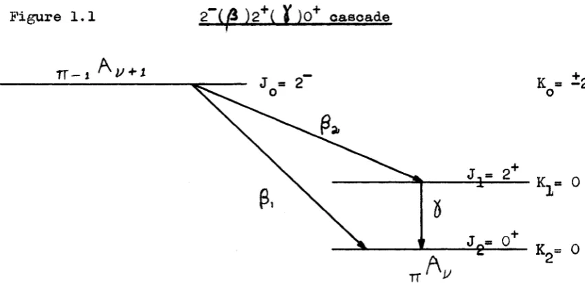
Figure 2.1 Decay Scheme of As74

TTTTT/SU7TT7T7

(~0.043&e)8.3

«

2220

(

0

.

02

$)

5 1600

(0.02J6)

600

8236

(2.8$£+j 2.2$£)

8.6

7777777

(s;

690

1636

7.5

^1635

(1636)

J^- 2

0

Se74 34 40

flotation.

32Ge42

Energy in kev.

($ of radiation)

log ft values.

Some useful formula's

p = E(E+2moc2 )

q » — (E - E)

W = E + m o°

or # of..Jag +

1

511 A

p2+l

m c o

w2

p (and q) ■ momentum of

fZ-vatf

W = Total energy of the electrons, Wq= max. energy of the electrons.

As74 E X P E R I M E N T

1. Apparatus

The angular correlation spectrometer used consisted of a

magnetic lens and two gamma spectrometers which could be rotated

with respect to the lens. The two gamma spectrometers were mounted

on the same arm with axis 90° apart. They were moved together using

the automatic scanning device (YOUNG.

64

90°

-l

80

used to separate the electrons from the positrons. (GERHOLM.) This

equipment has been described by COLCLOUGH. 63 and also by YOUNG.

64

In the present version the second gamma speotrometer was added to

the equipment described by YOUNG.

64

A block diagram of the electronic counting circuit is

shown in figure 2.2 and differs from the one previously described

in that a "two fold" fast coincidence circuit has been added. This

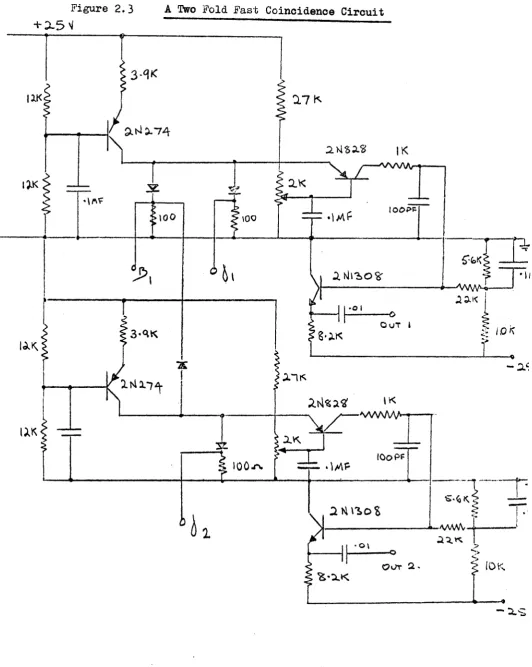
circuit is shown in figure 2.3. Short pulses ^ 1 0 n secs are

produced by the

404

^ and

^ 2

inputs

f3

j3

applied to the slow triple coincidence circuits, the output of which

go to the scalars. The system is essentially the same type as

described by BELL. GRAHAM. PETCH. 52, except, that the short pulses

are produced directly at the anodes of the

404

the rest of the circuits transistors are used instead of vacuum tubes.

When the T.M.C. kicksorter was used to observe the gamma

spectrum in coincidence with the betas, the fast coincidence pulses

figure 2 . 2 Block Diagram of Circuit Layout m

o

m

co

SLOW

FAST

SLOW

FAST

CO

o

> O CO

FAST

Figure 2.3 A Two Fold Fast Coincidence Circuit

+ 2-5

I IK

>00

Ou t >

32.

23

circuit, the beta pulses were applied to the third and the output

was used to gate the kicksorter.

To obtain the chance rate, the fast beta pulses were

delayed by ^ l O O n secs and the coincidence rates observed.

2. Source Preparation

A s ^ as sodium arsenate solution was obtained from "The

Radiation Biological Laboratories " Amersham, England. The specific

activity was greater than 120 mc/ml. A few drops of the solution

was evaporated to dryness in a tungsten boat using a heat lamp.

The boat was placed in a Balzer vacuum ooating unit. A substrate

of A1 of about 0.001 inches thickness was used and was placed

directly over the tungsten boat. A mask with a hole of 5®® in

diameter was placed against the substrate. The temperature of the

tungsten boat was raised slowly and the sodium arsenate evaporated

and condensed on the aluminum substrate.

3. Preliminary Adjustments

(i) Centering of the Source

The source was placed on the axis of the spectrometer

using the following method. A cylinder which fits snugly in the

vacuum chamber, and which has a small hole along its axis was placed

in the spectrometer. This hole was then on the axis of the instru­

ment. The source was then observed through this hole and adjusted

until it was centrally located.

(ii) Centering of the X Probe

The center of rotation of the gamma spectrometers were

adjusted to obtain equal count rates at the

90

Figure 2.4 The Gamma Singles Spectra

250

ANALYSER WITOOW

0.511 Mev. Annihilation Peak

200

0.596 Mev. and OJS35 Mev.

150

COUNTS SEC

100

0

300

400

500

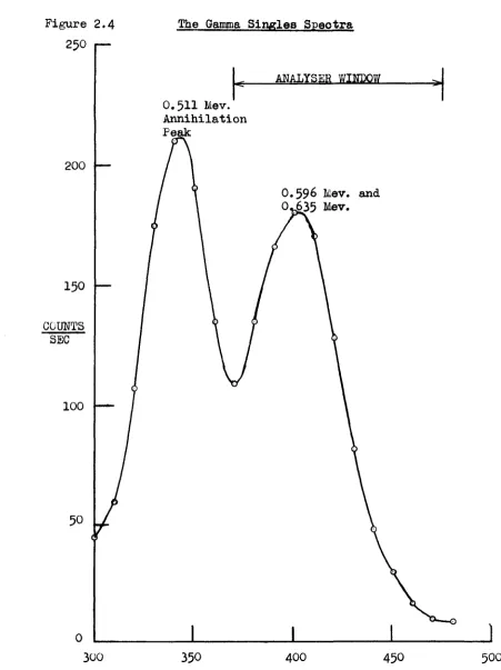
probe. The composite peak at 600 kev, see figure 2.4, was used.

The count rates were obtained equal to ~ 1 $ .

4. Experimental Procedures

Figure 2.1 shows the decay soheme of A s ^ . There are two

intense

j&~

p +

germanium are weakly fed < 0.1$ in this decay and are unimportant

in the experiment undertaken. The sequences 2~(

f3

~ decay and 2~(^tf+ )2+ (ft )0+ in the jg+ deoay were studied.

ie. The angular correlation between the 0.635 Mev gamma

ray and the ^ and the 0.590 Mev gamma ray and

the ^

Mev annihilation radiation, figure 2.4, contributed to the

X ~ %

scattered background, and not to the true coincidence. This

had to be excluded from the gamma channel and therefore the dis­

criminator windows were set to accept the composite peak as shown

in figure 2.4*

The equipment was set to record the gamma 1 singles, the

gamma 2 singles, the betas, the doubles, and the triple coincidences

due to ( y # ^ ) and (y£? <*a'fca was printed out and the

positions of the gamma spectrometers changed automatically every

twenty minutes. The equipment was interrupted every 12 hours and

the discriminator reset if necessary.

At the beginning and end of each such sequence, the chanoe

rate and the soattered ( $ ) background rate were recorded. To

obtain the

(X

- X

were closed and the coincidence rate recorded. The procedure was

repeated until more than

50

0°0

energy in the beta channel was then ohanged and the procedure

repeated.

5. Treatment of the Data

Since the anisotropy measured is very small it is impor­

tant to eliminate the effect of drifts in the gamma channel. This

is accomplished in two ways.

1/ The position of the counters were changed every twenty

minutes, which is an interval small enough for the drift to be

negligble.

2/ The magnitude of the drifts throughout a sequence was deter­

mined and the data rejected when necessay.

The following procedure was followed. The gamma spectrum

in coincidence with the betas was determined^figure 2.5 and figure

2.6. The count rate in the gamma channel as a function of the lower

discriminator setting was determined, using the window used in the

experiment, figure 2.7* From this graph, if the count rate in the

gamma channel is known, the spectrum shift could be read off

directly. The gamma channel rates in the experimental runs were

plotted as a function of time* M 0 H B M H I The straight solid line

passes through the 1st point and has the slope corresponding to the

half-life of A s ^ (l7»5 days). Deviation from this line indicated

drifts in the gamma channel. From the percentage deviation, the

shift of the spectrum was obtained using the graph in figure 2.8.

From the gamma spectra, figure 2.7, the corrections to the data

were obtained.

However, when the data deviated by as much as - 2

%

Figure 2,5 The Gamma 1 Spectra in Coinaidence with the Betas

ANALYSER WINDOW

600

COINCIDENCE

r a

COUNTS 12 hr

400

SCATTERING PEAK

200

^n-90'

COINCIDENCE ■fa PEAK

600

COUNTS 12 hr

400

200

SCATTERING PEAK

60

Figure 2.6 The Gamma 2 Spectra in coincidence with the Betas

-270° and l8o'

600

500

COINCIDENCE PEAK

400

COUNTS 12 hr

300

no scattering peak due to

511

200

100

0

50 55

40 ₄₅

Figure 2.7 $ change of # of peak counts,D, in gamma channel

versus change in Lower Discriminator

+15

change of N

+10

+5

+1

+2

%

Lower Discriminator -1

-10

Figure 2.8 $ change in coincidence count in same channel

versus

$

T +15

+10

change in coincidence counts

^ +1 +2

Jfe change in

Lower Discriminator

- 2

-10

gave the same values. It was therfore deoided to accept data

points which deviated -

1%

90

80

coincidence counts must be corrected for this peak shift. The

percentage difference in position between the two peaks is deter­

mined, then the coincidence count for the higher peak must be

reduced by a certain amount determined from figure

2

8

TABLE III

Asymmetry, A

2

Corrections for Hegatrons

Energy Asymmetry, a(w) a

2

Baffles Baffles Baffles Baffles for for

Y+fi

W

6

6

Open Open Open Open Angle Angle

1.6

0.0098

0.012

-

0.005

1.8

488

0.0261

45

± 0.006

2.0

i

0.006

p To correct for

j3

_2

Po

P 2

for Baffles 6 turns open » 0.7612 - 0,003 o

P2

for Baffles 7 turns open •p— * 0.7453 - 0.003

To correct for $ spectrometer solid angle divide A

2

TABLE IV

Asymmetry, Ag Coefficient and Solid Angle

Corrections for Positrons

Energy Asymmetry

a(w)

A2

Corrected

For

jB

Solid

Angle

Corrected

For

X+P

Solid

Angle

Ag (Corrected)

Average

For Both

Counters

(a)

y

1.8

2.0

2.1

2.2

0.0256

0.01692

0.01606

0.01322

0.03118

0.02178

0.01360

0.02238

(b)

X

1.8

2.0

2.1

2.2

2

0.0181

0.0151

0.0288

0.0306

0.01001

0.01901

0.02019

0.01626

0.01680

0.01406

0.015

0.006

0.019 - 0.004

0.030

t

0.005

0.025

0.005

To correct for

f3

for baffles 7 turns open * 0.7372 -

0.008

To correct for

%

(for 10 cm away and l

^ 11

Corrections for Chance and Scattering

P 0 S I T B 0 N 3

Energy A ? Coinc Counts : Chance Counts< Coinc Counts : Scattering Counts ^

W

_*2

X 2-210°

1.8 0.0136 0.0168 -.0

80:1

80:1

-

-

0.004

2.0 0.0236 0.0141 160:1 160:1 160:1 160:1 100:1

70:1

90:1

-

0.0028

-

2.1 0.0323 0.0267 :0 :0 :0 :0

70:1

70:1

i

0.0033

-

2.2 0.0224

0.0284

150:1

170:1

-

0.0031

-

H e

a

1.6 0.0120 6:1 6:1 Corrected for Scattering in Analysis

-

0.005

1.8 -0.0451 3:1 3:1 3:1 3:1

- 0.006

2.0 _-0.0445 3:1 3:1 2:1 2:1

-

TABLE VI

P O S I T R O N S

Table of Coinoidenoes to Get a(w)

Energy

(w)

180

180

2.0

44 9417 9455 1.0374

1.0232

46

.9684

47 4693 4841

1.0100

0.9801

C

M

12034 12029 1.0227

1.0125

0.9900

45 12845

12872

1.0246

46

11301

1.0121

.9856

47

6316

0,9812

2.1

_{* 1}

49 5984

6074

0.9890

96

50 5906 ₅₉₆₅ 1.0207

0.9850

965

52

V

1195

1162

1.0361

1.0002

c>2

48 7492 7650 1.0157 0.9872 0.9719

49

6815

84

50 6911 6967

1.0221

51

5611

1.0211

2.2

_{^ 1}

53 3871 3817

1.0298

1.0510

1.0205

54

4010

1.0270

55

3060

588

0.9766

56

1.0148

57 3173 3129

1.0502

58

y

3769 3981 1.0597 0.9894 0.9336

0

2

54 55 56 57 58 4416 3918 2940 3381 4175 4499

4018

.0246

98

.9894

.9949

O.

97

0.9682

O

.9642

.9846

1.8

h

59 2429

2460

1.0116

.9685

60

2281

62

64

Y

1319 1238 1.0717

1.0784

1.0062

6

2

60

2801

1.0071

61

63 2104

2150

1.0021

0.9688

0.9667

64 1340 1319

0.9900

1.0060

... .

The ratio ^ — corrected for difference in position of

o l80° o peak between

90

180

coinc

90

80

scattering.

However, in TABLE VII, coinc 90° and coinc 180° are corrected for

TABLE VII

N E G A T R O N S

Table of Coincedences to Get a(w)

Energy (w) Seq # Coinc 90° Coino 180° Normalizing Factor 180? "90° .... ~

180° „ Norm.

90

1.6 1 5152 4945 0.9598

3 7588 7492 0.9873

'1

.0147

4 8394 8261 O.

984

5

6655

6685

j

6 3813 3685 O

.9664

[

8 3007 2991

1.0288

1.8 12 3630 3376 1.0310 0.9300 O

.9588

13 3656 3347 1.0380 0.9155 0.9503

14 2971 2711 1.0330 0.9125 0.9426

15 5417 4995 1.0320

0.9221

.9516

16 2254 2172 1.0392 0.9636 1.0014

17 1877 1729 1.0318

0.9212

18 2000 ₁₈₅₉ 1.0296 0.9295 0.9570

20 723 694 1.0347 0.9599 0.9932

21

828

0.8225

0.8490

22 3747 3477 1.0257 0.9279 0.9518

23 1666 1591 1.0309 0.9550 0.9845

2.0 30 2504 2222 1.0353

0.8874

0.9187

31 3892 3608 1.0338

0.9270

0.9583

32

3028

2846

0.9697

33 3327 3081 1.0374 0.9261

0.9607

34 2515 2334 1.0360 0.9280

0.9614

35

1142

46

0.9454

37 2577 2499 1.0445 0.9697

1.0129

38 1753 1661 1.0290 0.9475

0.9750

39 205 181 1.0142 0.8829

0.8954

411, 754

685

0.9085

0.9215

*2 995 994 1.0361 0.9487

0.9829

CHAPTER III

Interpretation of Results and Conclusions

1. The Shell Model

Prom TABLE VIII of the Shell model and from Nuclear data

*7 A

on As (Ref. Fig. 2.1) the reaction that takes place seems to he

of two definite forms.

(i) As*^ A t t =

-1

UJ

~

^

P

+ 34 4°

*7 A

As has 33 protons and 41 neutrons; the last odd proton

is in the If,- state and the last odd neutron is in the

1st

1

1

2 2

An electron (|@ ) is given off by A s ^ to produce Se^^ which has

34 protons and 40 neutrons. When the electron is given off (from

eqn l.l), one neutron disappears and is replaced by a proton. The

extra proton also goes into the If” state and combines with the

1

other proton already there to form an even-even nucleus or a

STABLE ELEMENT.

i ■

74

> f

3

a

positron

(j£+)

32

is replaced by a neutron^from the eqn

1

2

into the lg^ state and combines with the neutron that was already

2

there and thus an even-even (STABLE) nucleus is formed. In this

model a nucleon is transformed from a If” to a lg* state when ^

0

2

2

2 2