A diagonal preconditioner for singularly perturbed problems

(1)

R E S E A R C H

Open Access

A diagonal preconditioner for singularly

perturbed problems

Dana ˇCerná and Václav Fin ˇek

*

Department of Mathematics and Didactics of Mathematics, Technical University of Liberec, Studentská 2, Liberec, 461 17, Czech Republic

Abstract

Using wavelet discretization with a standard wavelet diagonal preconditioning for singularly perturbed two-point boundary value problems, one can observe that condition numbers of arising stiﬀness matrices are growing with decreasing parameter

when a nonsymmetric part starts to dominate. We propose here a simple diagonal preconditioning which significantly improves condition numbers of the stiffness matrices with a dominating nonsymmetric part and compare it with a standard wavelet preconditioning. Further, we prove that the condition numbers of diagonally preconditioned stiffness matrices are bounded independent of the matrix size. Numerical examples are given.

MSC: 65L11; 65L10; 65T60; 65F08

Keywords: wavelets; singularly perturbed problems; boundary value problems; preconditioning

1 Introduction

Many problems in science and technology can be modeled by boundary value problems for singularly perturbed differential equations. Singularly perturbed problems arise for example in the modeling of fluid flow at high Reynolds numbers, water quality problems in river networks, convective heat transport problems with large Peclet numbers, drift diffusion equations of semiconductor device modeling, simulation of oil extraction from under-ground reservoirs, theory of plates and shells, atmospheric pollution, groundwater transport, and chemical reactor theory. For a detailed survey of different applications, we refer to []. Recently also singularly perturbed semilinear boundary value problems with discontinuous coefficients and nonlinear reaction-diffusion equations attracted some at-tention; see [, ] and the references therein. A vast majority of these problems cannot be solved analytically and therefore it is necessary to solve them approximately. In the mod-eling of the above processes, one can observe boundary and interior layers whose width can be arbitrarily small.

We consider here the following singularly perturbed two-point boundary value problem:

–u(x) +p(x)u(x) +q(x)u(x) =f(x) ∀x∈(, ) ()

withu() = ,u() = , ()

(2)

where  <  is a parameter,p∈C_{[, ],}_q_∈_C_{[, ],}_f _∈_C_{[, ], and}_p₍_x_{) >}_α_{> .} Then the above problem has a unique solutionu(x) []. This equation represents a simple mathematical model of a convection-diﬀusion problem and it can be used to model many practical problems. For example the linearized Navier-Stokes equations at high Reynolds number provide an accurate model of the transition dynamics in the problem of turbu-lence suppression in channel ﬂow. Problems of these types have solutions which are dis-continuous asis approaching zero and typically possess boundary or interior layers,i.e.

regions of rapid change in the solution near the endpoints or some interior points. There-fore, it is usually more diﬃcult to solve them for very small parameter. Many numerical methods have been suggested to solve such types of problems and a lot of them require information as regards locations and widths of diﬀerent layers. One of the possibilities to solve them without this information is an application of adaptive methods.

In recent years, there have appeared some promising results in using wavelets to solve singularly perturbed problems. In [], a non-adaptive numerical method based on wavelets of Hermite cubic splines was presented and improved results were obtained in comparison with other techniques. In [], the authors constructed wavelets of order  with five vanishing wavelet moments with respect to which stiffness matrices for ordi-nary differential equations with constant coefficients are very sparse (in comparison with other kinds of wavelets) and their condition numbers are similarly small as in [] for lower order wavelets. Then they applied tensor product wavelets to the adaptive solution of a reaction-diffusion equation in two space dimensions.

In this contribution, we focus on methods based on wavelets. Using wavelet discretiza-tion with a standard wavelet diagonal precondidiscretiza-tioning for singularly perturbed two-point boundary value problems, one can observe that the condition numbers of arising stiﬀness

matrices are growing with decreasing parameterwhen a nonsymmetric part starts to

dominate. In the wavelet methods, the continuous problem is transformed into a well-conditioned discrete problem. And once a well-well-conditioned nonsymmetric problem is given, squaring will yield a symmetric positive definite formulation []. Therefore an ef-ficient preconditioning is very important since the rate of convergence for most iterative linear solvers depends on the condition number of a preconditioned matrix. We propose here a simple diagonal preconditioning which significantly improves the condition num-bers of the stiffness matrices with a dominating nonsymmetric part. A diagonal precondi-tioning is optimal for adaptive wavelet methods in which often stiffness matrices are not explicitly assembled and not stored in a computer memory. This paper is organized as follows: First, we briefly introduce wavelet bases and their properties. Then we propose a new diagonal preconditioning and we prove that the condition numbers of the infinite diagonally preconditioned stiffness matrices are finite. At the end, we provide some nu-merical examples.

2 Wavelet bases

We consider here families={ψλ,λ∈J} ⊂L(, ) of functions (wavelets) that are nor-malized inL(, ) such thatψλL(,)= . LetJ be an inﬁnite index set andJ =J∪J,

whereJis a ﬁnite set representing scaling functions living on the coarsest scale. Any in-dexλ∈J is of the formλ= (j,k), where|λ|=jdenotes a scale andk denotes spatial location. Further, we will denote Dsa diagonal matrix, whose diagonal entries are s|λ|_. Then D–s₌_{_–s|λ|_ψ

(3)

to write wavelet expansions as

dT:= λ∈J

dλψλ.

At last, fors≥ the spaceHs_{will denote a closed subspace of the Sobolev space}_Hs_{(, ),}

deﬁnede.g.by imposing homogeneous boundary conditions at one or both endpoints, and fors<  the spaceHswill denote the dual spaceHs:= (H–s). · Hs will denote the

cor-responding norm. Furtherl(J) will denote the space consisting of the power summable sequences and · l(J)will denote the corresponding norm.

A family={ψλ,λ∈J} ⊂L(, ) is called awavelet basisofHsfor someγ,γ>  and

s∈(–γ,γ), if:

• is a Riesz basis ofHs_{, which means}_{forms a basis of}_Hs_{and there exist constants}

cs,Cs> such that for allb={bλ}λ∈J ∈l(J)we have

csbl_(J)≤bTD–s_Hs≤Csbl(J), ()

wheresupcs,infCsare called Riesz bounds andcond:=infsupCcss is called the condition

number of.

• Functions are local in the sense thatdiam(suppψλ)≤C–|λ|for allλ∈J, whereCis a constant independent ofλ.

• Functionsψλ,λ∈J, have cancellation properties of orderm,i.e.

_v(x)ψλ(x)dx

≤–m|λ|_|_v_|H

m_(,), ∀v∈Hm(, ).

It means that integration against wavelets eliminates smooth parts of functions and it is equivalent with vanishing wavelet moments of orderm.

Norm equivalences () have the following important consequence which will be used later.

Theorem  Let H be a Hilbert space, ·,·:H×H→R,and suppose that there exist constants c,C> such that

cbl_(J)≤bT_H≤Cbl(J) ∀b∈l(J) ()

i.e.,is a Riesz basis of H.Then

C–,b_l

(J)≤ bH≤c

–_,_b

l(J) ∀b∈H

_. _()

For the proof, we refer to [].

The application of wavelets for the numerical solution of diﬀerential equations has sev-eral advantages, namely:

• Vanishing wavelet moments (the cancellation property) lead to sparse representations of functions and operators.

(4)

function inHs_{has a unique expansion in the scaled wavelet basis and that there is a}

tight relation between the function norms and wavelet coeﬃcients. It means that small changes in wavelet coeﬃcients can cause only small changes in the function and the other way around. Wavelet bases with small Riesz bounds were constructed for example in [–].

• There are wavelet-based asymptotically optimal algorithms for solving elliptic PDEs. See for example [–]. It means that the number of ﬂoating point operations depends linearly on the number of nonzero wavelet coeﬃcients.

3 Wavelet discretization

We restrict ourselves to the equation –u+bu+cu=f with the Dirichlet boundary con-ditionsu() =u() = , with small positive parameterand with constantsb,c> . Now, this continuous problem can for suitable wavelet bases be transformed into an equivalent well-conditioned problem inl. We start with the standard variational formulation: Find

u∈H

(, ) such that

a(u,v) =f(v), ∀v∈H_(, ), ()

where a bilinear forma:H

(, )×H(, )→Randf ∈H–(, ) are given by

a(u,v) := 



uvdx+ 



buv dx+ 



cuv dx, f(v) := 



fv dx. ()

Now, we deﬁne an operatorA:H

(, )→H–(, ) by

u,Av=a(u,v), u∈H_(, ), ()

and then () is equivalent with the task: for givenf∈H–_{(, ) ﬁnd}_u_∈_H

(, ) such that

Au=f. ()

The scaled representation of () and the scaled wavelet representation of the right-hand side are then given by

A:= D–_A,AD–_A, F:= D–_Af(),

where DAis an appropriate diagonal matrix which will be speciﬁed later. Suppose that

u= uT_D–_{is the scaled wavelet representation of the solution, then}

Au=f ⇐⇒ Au= F. ()

For more details, we refer to [].

First, we prove that the problem () is well posed in energy norm. The spaceH–(, ) is endowed with the norm

|||Av|||= sup

u∈H

u,Av

|||u||| .

(5)

Theorem  The variational problem()is well posed on H

(, )equipped with energy

norm|||v|||_:=

(v)dx+ 

cvdx in the sense that

|||v||| ≤ |||Av|||≤

 +√b

c |||v||| ∀v∈H

 (, ).

Proof Foru,v∈H

(, ), we have

u,Av=a(u,v)

= 



uvdx+ 



buv dx+ 



cuv dx

≤uv+buv+cuv

≤√u√v+√u√cv√b c+

√

cu√cv

≤

 +√b

c+  |||v||||||u|||

and

|||v||| = 



vdx+ 



b



vdx+ 



cvdx

= 



vdx+ 



bvv dx+ 



cvdx

=v,Av

=|||v|||v,Av

|||v|||

≤ |||v|||sup

u∈H 

u,Av

|||u||| =|||v||||||Av||| _.

Then

|||v||| ≤ |||Av|||=sup

u∈H

u,Av

|||u||| ≤

( +√b

c)|||v||||||u||| |||u||| =

 +√b

c |||v|||.

Then the operatorAis bounded and coercive and an application of the Lax-Milgram

lemma implies the existence of the unique solution for anyf ∈H–_{(, ). Further, we prove} that a diagonally scaled wavelet basis is a Riesz basis when it is scaled with the proposed diagonal scaling.

Theorem  LetDA:= (

(|λ|₊_b_|λ|₊_c₎_δ

λ,μ)be the diagonal matrix,,b,c be positive

constants and let the norm equivalences()hold forγ > .Then for everyu∈l(J)there

exist positive constants c,c,C,Csuch that

min{c,c}

max{( +_b), ( +_b_c)}

(6)

Proof Let us denoteu= vT_{= (D}

Av)TD–A, u = DAv, and v ={vλ}l(J). Then the norm

equivalences () and Frie drichs’ inequality imply that there exist positive constantsc,c,

C,Csuch that

c

λ∈J |λ|_v

λ≤u 

≤C

λ∈J |λ|_v

λ and c

λ∈J

v_λ≤ u≤C

λ∈J

v_λ.

Using these inequalities, we obtain

|||u|||≤C_Dv_l (J)+C



cvl(J) ≤maxC_,C_

λ∈J

|λ|+cvλ

≤maxC_,C_

λ∈J

|λ|+b|λ|+cvλ=max

C_,C_ul_(J)

and

u_l

(J) =DAv

 l(J)

=

λ∈J

|λ|₊_b_|λ|₊_c_v λ



l(J)

=

λ∈J

|λ|₊_b_|λ|₊_c_v λ

≤

λ∈J

|λ|₊b 

 + |λ|₊

c vλ

=

λ∈J

+b

 

|λ| +

c+b 

vλ

=

λ∈J

 + b

 

|λ| +c

 + b

c

vλ

≤max

 + b

 ,

 + b

c

λ∈J

|λ|+cvλ

≤maxc–_ ,c–_ max

 + b

 ,

 + b

c |||u|||

_.

And finally we prove that the condition numbers of the infinite diagonally precondi-tioned stiffness matrices are finite.

Theorem  LetDA:= (

(|λ|₊_b_|λ|₊_c₎_δ

λ,μ)be the diagonal matrix,,b,c be positive

constants and let the norm equivalences()hold forγ > .Then

cond(A) :=condD–_A,AD–_A

≤ max{C 

,C}( +√bc)

min{c

,c}(max{( +b), ( + b c)})–

,

(7)

Proof Using Theorems , , and  implies

minc_,c_max

 + b

 ,

 + b

c

– ul_(J)

≤min{c,c}

max

 + b

 ,

 + b

c

–/ |||u|||

≤min{c,c}

max

 + b

 ,

 + b

c

–/ |||Au|||

≤D–_A,Au_l (J)

=D–_A,AD–_Au_l (J)

=Aul_(J)

≤max{C,C}|||Au|||

≤max{C,C}

 +√b

c |||u|||

≤maxC_,C_ +√b

c ul(J).

Remark  From the previous theorem it immediately follows that, forb= , we obtain

symmetric stiﬀness matrices with small condition numbers which are independent of

and are dependent only on Riesz constants of the used wavelet basis.

4 Numerical tests

In adaptive settings the discrete infinite-dimensional problem () is solved approximately up to the given target accuracy. Adaptive wavelet methods are meshless methods. An adaptive algorithm usually starts with the zero function and gradually adds new (biggest) elements to approximate () and then only a part of the whole stiffness matrix is used. While in non-adaptive settings, we compute with all wavelets up to the given level. In numerical experiments, we use the second approach because it is more appropriate for comparison of the properties of the wavelet stiffness matrices.

As basis functions, wavelets proposed in [] are used because they have vanishing mo-ments, short support, are well conditioned, and, finally, for constant coefficient differen-tial equations, the arising stiffness matrices are sparse in wavelet coordinates. In the usual case they are only quasi-sparse. These wavelets are based on Hermite cubic splines. Primal scaling functions are defined by

φ(x) = ⎧ ⎪ ⎪ ⎨ ⎪ ⎪ ⎩

(x+ )_{( – }_x_), _–_≤_x_≤_,

( –x)_(_x_{+ ),} __≤_x_≤_,

 otherwise,

φ(x) = ⎧ ⎪ ⎪ ⎨ ⎪ ⎪ ⎩

(x+ )_x_, _–_≤_x_≤_,

( –x)x, ≤x≤,

(8)

Forn≥, letVnbe the space of piecewise cubic splinesv∈C(, )∩C[, ] for which

v() =v() = . The dimension ofVnis n+and the set

n:=

φ

nx–j:j= , . . . , n– ∪φ

nx–j|[,]:j= , . . . , n

is the basis forVn. LetWnbe the complement ofVninVn+then we have the following decomposition of spaceH

(, ):

H_(, ) =V⊕W⊕W⊕W· · ·.

Four types of wavelets,ψ,ψ,ψ, andψ, are constructed and the wavelet basis is then formed by translations and dilations of these four types of wavelets. Wavelets from the spaceWn+are orthogonal to the scaling functions from the spaceVnforn≥. The ﬁrst

two wavelets have supports in [–, ] and are uniquely determined by the above orthog-onality condition and by imposing that the ﬁrst one is odd and the second one is even. The second two wavelets have supports in [–, ]. And we impose again the orthogonality condition and one of them should be odd and the second one even. This property ensures that both the mass and the stiﬀness matrix corresponding to the one-dimensional Lapla-cian have at most three wavelet blocks of nonzero elements in any column and then the number of nonzero elements in any column is bounded independent of matrix size.

Then a basis of the spaceWnis deﬁned as follows:

n:=

ψ

nx– j– ,ψ

nx– j– :j= , . . . , n–– 

∪ψ

nx– j:j= , . . . , n–– 

∪ψ

nx– j|[,]:j= , . . . , n–

.

In the following part, we assume that all basis functions are normalized with respect to theLnorm, such that their norm is equal to one. Now, we look at the spectral properties of diﬀerent stiﬀness matrices An. We will use the standard wavelet preconditioning with

the diagonal preconditioner DS n=

diag(An) [] and then we will compare it with the

proposed diagonal preconditioning Dnew n := (

(|λ|₊_b_|λ|₊_c₎_δ

λ,μ), where the constants

,b,care constants from ().

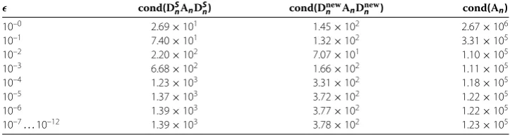
Example  We start with the equation –u+u+u/ =f with the Dirichlet boundary conditionsu() =u() =  and with small positive parameter. The corresponding dis-crete problem is the following:

Findun=

n+

i= civi, wherevi∈∪nj=j, such that





u_nv+u_nv+unv/dx= 



fv dx ∀v∈∪ n

j=

j

or in matrix form Ancn= fn, where Anis the stiﬀness matrix corresponding to the above

equation and fnis the corresponding vector of the right-hand side. The obtained results

(9)

Table 1 The condition numbers of the stiffness matrices forn= 9

cond(DS

nAnDSn) cond(DnnewAnDnewn ) cond(An)

10–0 _2.69_×₁₀1 _1.45_×₁₀2 _2.67_×₁₀6

10–1 _7.40_×₁₀1 _1.32_×₁₀2 _3.31_×₁₀5

10–2 _2.20_×₁₀2 _7.07_×₁₀1 _1.10_×₁₀5

10–3 _6.68_×₁₀2 _1.66_×₁₀2 _1.11_×₁₀5

10–4 _1.23_×₁₀3 _3.31_×₁₀2 _1.18_×₁₀5

10–5 _1.37_×₁₀3 _3.72_×₁₀2 _1.22_×₁₀5

10–6 _1.39_×₁₀3 _3.77_×₁₀2 _1.22_×₁₀5

10–7_{. . .}₁₀–12 _1.39_×₁₀3 _3.78_×₁₀2 _1.23_×₁₀5

cond(DS

10–0 _1.47_×₁₀2 _3.67_×₁₀1 _6.27_×₁₀6

10–1 _1.12_×₁₀3 _7.27_×₁₀1 _8.17_×₁₀5

10–2 _3.95_×₁₀3 _6.46_×₁₀1 _2.75_×₁₀5

10–3 _2.94_×₁₀4 _1.24_×₁₀2 _2.78_×₁₀5

10–4 _6.30_×₁₀4 _2.07_×₁₀2 _1.87_×₁₀5

10–5 _6.41_×₁₀4 _2.03_×₁₀2 _1.57_×₁₀5

10–6 _6.41_×₁₀4 _2.03_×₁₀2 _1.55_×₁₀5

10–7_{. . .}₁₀–12 _6.41_×₁₀4 _2.03_×₁₀2 _1.54_×₁₀5

Example  The second equation will be –u+u=f with the Dirichlet boundary con-ditionsu() =u() =  and with small positive parameter. The corresponding discrete problem is the following:

Findun= n+

i= civi, wherevi∈∪ n

j=j, such that





u_nv+u_nv dx= 



j=

j

equation and fnis the corresponding vector of the right-hand side. The obtained results

are summarized in Table .

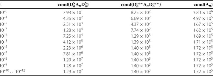
Example  The third equation will be –u+u+x_u₌_f_{with the Dirichlet boundary} con-ditionsu() =u() =  and with small positive parameter. The corresponding discrete problem is the following:

Findun= n+

i= civi, wherevi∈∪ n

j=j, such that





u_nv+u_nv+xunv dx= 



j=

j

equation and fn is the corresponding vector of the right-hand side. In this case of the

diﬀerential equation with variable coeﬃcients, we takec=  becausex_≤__∀_x_∈_{[, ].} The obtained results are summarized in Table .

5 Conclusion

(10)

cond(DS

10–0 _7.93_×₁₀1 _8.25_×₁₀2 _3.80_×₁₀6

10–1 _4.26_×₁₀2 _6.69_×₁₀2 _4.97_×₁₀5

10–2 _2.31_×₁₀3 _4.37_×₁₀2 _1.67_×₁₀5

10–3 _1.28_×₁₀4 _7.74_×₁₀2 _1.62_×₁₀5

10–4 _7.25_×₁₀4 _1.29_×₁₀3 _1.69_×₁₀5

10–5 _4.12_×₁₀5 _1.39_×₁₀3 _1.71_×₁₀5

10–6 _2.23_×₁₀6 _1.40_×₁₀3 _1.72_×₁₀5

10–7 _7.81_×₁₀6 _1.40_×₁₀3 _1.72_×₁₀5

10–8 _1.20_×₁₀7 _1.40_×₁₀3 _1.72_×₁₀5

10–9 _1.28_×₁₀7 _1.40_×₁₀3 _1.72_×₁₀5

10–10_{. . .}₁₀–12 _1.29_×₁₀7 _1.40_×₁₀3 _1.72_×₁₀5

leads to significantly smaller condition numbers of stiffness matrices with a dominating nonsymmetric part in comparison with a standard wavelet diagonal preconditioning. Fur-thermore, we proved that the condition numbers of diagonally preconditioned stiffness matrices are bounded independent of the matrix size.

Competing interests

The authors declare that they have no competing interests. Authors’ contributions

All authors contributed equally to the writing of this paper. All authors read and approved the ﬁnal manuscript. Acknowledgements

This work was supported by grant No. GA16-09541S of the Czech Science Foundation.

Received: 21 October 2016 Accepted: 27 January 2017

References

1. Kadalbajoo, MK, Gupta, V: A brief survey on numerical methods for solving singularly perturbed problems. Appl. Math. Comput.217, 3641-3716 (2010)

2. Bisci, GM, Repovš, D: On some variational algebraic problems. Adv. Nonlinear Anal.2, 127-146 (2013)

3. Nie, D, Xie, F: Singularly perturbed semilinear elliptic boundary value problems with discontinuous source term. Bound. Value Probl.2016, 164 (2016). doi:10.1186/s13661-016-0673-9

4. Gartland, EC Jr.: An analysis of a uniformly convergent finite difference/finite element scheme for a model singular-perturbation problem. Math. Comput.51, 93-106 (1988)

5. Chen, X, Xiang, J: Solving diﬀusion equation using wavelet method. Appl. Math. Comput.217, 6426-6432 (2011) 6. Chegini, N, Stevenson, R: The adaptive tensor product wavelet scheme: sparse matrices and the application to

singularly perturbed problems. IMA J. Numer. Anal. (2011). doi:10.1093/imanum/drr013

7. Dijkema, TJ, Stevenson, R: A sparse Laplacian in tensor product wavelet coordinates. Numer. Math.115, 433-449 (2010)

8. Bramble, JH, Cohen, A, Dahmen, W: Multiscale problems and methods in numerical simulations. In: Canuto, C (ed.) Lecture Notes in Mathematics. C.I.M.E. Foundation Subseries, vol. 1825, pp. 1-170. (2003)

9. ˇCerná, D, Fin ˇek, V: On a sparse representation of an-dimensional Laplacian in wavelet coordinates. Results Math.69, 225-243 (2016)

10. ˇCerná, D, Fin ˇek, V: Construction of optimally conditioned cubic spline wavelets on the interval. Adv. Comput. Math.

34, 219-252 (2011)

11. ˇCerná, D, Fin ˇek, V: Cubic spline wavelets with complementary boundary conditions. Appl. Math. Comput.219, 1853-1865 (2012)

12. ˇCerná, D, Fin ˇek, V: Quadratic spline wavelets with short support for fourth-order problems. Results Math.66, 525-540 (2014)

13. ˇCerná, D, Fin ˇek, V: Cubic spline wavelets with short support for fourth-order problems. Appl. Math. Comput.243, 44-56 (2014)

14. ˇCerná, D, Fin ˇek, V: Wavelet basis of cubic splines on the hypercube satisfying homogeneous boundary conditions. Int. J. Wavelets Multiresolut. Inf. Process.13(2015). doi:10.1142/S0219691315500149

15. Cohen, A, Dahmen, W, DeVore, R: Adaptive wavelet schemes for elliptic operator equations - convergence rates. Math. Comput.70, 27-75 (2001)

16. Cohen, A, Dahmen, W, DeVore, R: Adaptive wavelet methods II - beyond the elliptic case. Found. Comput. Math.2, 203-245 (2002)