http://www.sciencepublishinggroup.com/j/ajtas doi: 10.11648/j.ajtas.20170605.12
ISSN: 2326-8999 (Print); ISSN: 2326-9006 (Online)
Performance Rating of the Exponentiated Generalized
Gompertz Makeham Distribution: An Analytical Approach
Ogunde Adebisi Ade
1, Fatoki Olayode
2, Ajayi Bamidele
11
Department of Mathematics and Statistics, The Federal Polytechnic Ado-Ekiti, Ado-Ekiti, Nigeria
2Department of Statistics, Ogun State Institute of Technology, Igbesa, Nigeria
Email address:
To cite this article:
Ogunde Adebisi Ade, Fatoki Olayode, Ajayi Bamidele. Performance Rating of the Exponentiated Generalized Gompertz Makeham Distribution: An Analytical Approach. American Journal of Theoretical and Applied Statistics. Vol. 6, No. 5, 2017, pp. 228-235. doi: 10.11648/j.ajtas.20170605.12
Received: April 22, 2017; Accepted: May 2, 2017; Published: September 4, 2017
Abstract:
We developed a five parameter distribution known as the Generalized Exponentiated Gompertz Makeham distribution which is quite flexible and can have a decreasing, increasing and bathtub-shaped failure rate function depending on its parameters making it more effective in modeling survival data and reliability problems. Some comprehensive properties of the new distribution, such as closed-form expressions for the density function, cumulative distribution function, hazard rate function, moment generating function and order Statistics were provided as well as maximum likelihood estimation of the Generalized Exponentiated Gompertz Makeham distribution parameters and at the end, in order to show the distribution flexibility, an application using a real data set was presented.Keywords:
Generalized Exponentiated Gompertz Makeham Distribution, Maximum Likelihood Estimation, Bathtub-Shape Failure Rate, Distribution Flexibility1. Introduction
Generalized Exponentiated Class of distribution
Cordeiro G. M. et al. Proposed a new method of adding two shape parameters to a continuous distribution that extends an idea which was first introduced by Lehmann and studied by Nadarajah and Kotz. The idea produces a new class of exponentiated generalized distributions that can be interpreted as a double construction of Lehmann alternatives. Given a continuous cumulative density function, G. M Cordeiro et al define the exponentiated generalized class of distribution by
1 1 (1) And the probability density function given by
1 (2)
Where are two additional shape parameters in equations can control the both the tail weight and possibly adding entropies to the center of the exponentiated generalized density function.
2. Gompertz Makeham Distribution
The Gompertz distribution was first introduced by Benjamin Gompertz a British actuary. The distribution has been used frequently to describe human mortality, growth model and actuarial tables.
A different version of Gompertz distribution which is called Gompertz Makeham (GM) distribution was introduced by another British actuary, Makeham. He introduced a constant (Makeham terms) that describe the age independent mortality and has received considerable attention in the literature. The GM family has been studied by Baily et al. and an expression using the Lambert W function for the quantile function was given by Jodra, P. Suppose now is a GM random variable with the cumulative density function given by
+ , ", > 0 (4)
According to Finch, the Gompertz Makeham distribution produces a better fit between the age windows 30 to 85 years. An extension of the distribution will induce flexibility and enable it to cope with early failure or infant mortality.
3. The Proposed Generalized
Exponentiated Gompertz Makeham
Distributions
Putting (3) in (1), the cumulative density function of generalized exponentiated Gompertz Makeham (EGGM)
distribution can be obtained as follows
%1 − & '( (5)
The graph below depicts the behaviour of the Cumulative density function of the EGGM distribution.
Also putting (4) in (2), we obtain an expression for the probability density function of the Generalized Exponentiated Gompertz Makeham (EGGM) distribution as follows
= + & '%1 − & '( (6)
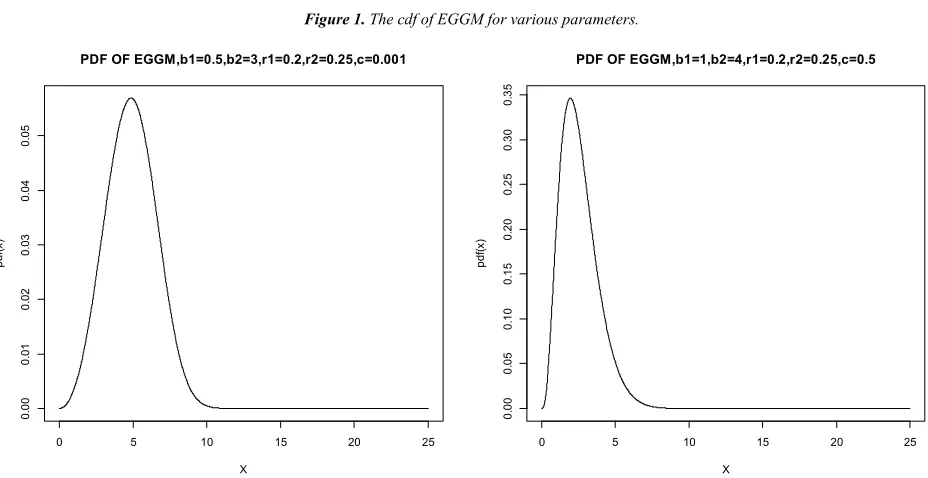
The graph below depicts the behaviour of EGGM at different values of the shape parameters.
Figure 1. The cdf of EGGM for various parameters.
Figure 2. The pdf of EGGM for various parameters.
0 5 10 15
0
.0
0
.2
0
.4
0
.6
0
.8
1
.0
CDF OF EGGM,b1=2.5,b2=3,r1=0.2,r2=0.25,c=0.1
X
c
d
f(
x
)
0 5 10 15
0
.0
0
.2
0
.4
0
.6
0
.8
1
.0
CDF OF EGGM,b1=1,b2=4,r1=0.2,r2=0.25,c=0.5
X
c
d
f(
x
)
0 5 10 15 20 25
0
.0
0
0
.0
1
0
.0
2
0
.0
3
0
.0
4
0
.0
5
PDF OF EGGM,b1=0.5,b2=3,r1=0.2,r2=0.25,c=0.001
X
p
d
f(
x
)
0 5 10 15 20 25
0
.0
0
0
.0
5
0
.1
0
0
.1
5
0
.2
0
0
.2
5
0
.3
0
0
.3
5
PDF OF EGGM,b1=1,b2=4,r1=0.2,r2=0.25,c=0.5
X
p
d
f(
x
The graph drawn above indicates that the pdf of EGGM is positively skewed
3.1. Expansion for the Density Function
For any real non integer b, we consider the binomial series,
1 − ) = ∑, −1 +
+-. + )+ (7)
Which is valid for |)| < 1
Applying equation (7) in (5), we have
= ∑, −1 1
1-. 213 & '1 (8)
Also for the probability density function we have
= + & '∑, −11
1-. 213 & '1 (9)
Finally we have
= ∑, −11
1-. 2 1 3 & ' 4 1 (10)
3.2. Verification of Exponentiated Generalized Distribution to Be a Proper Pdf
Here, we want to show that the integral of the EGGM distribution equal to 1; that is
5,, = 1 (11)
5,, = 5,, + & '%1 −
& '( 6
(12)
Let 7 = , then
67 = − + ,
this implies that6 = 4:89 9 substitute this in equation
(12), we have
;
,
,
= ; + 7 1 − 7 +67 7
,
,
On simplification this gives
5,, = 5,,7 1 − 7 67 (13)
Further if we let < = 7 , 6< = 7 67, 67 = 98=>?@, substitute this in equation (13), we have
;
,
,
= ; A< B 1 − < 6<
A< B ,
,
,
Finally we have
;
,
,
= ; 1 − < 6< = 1
,
,
This verified that the pdf of EGGM distribution function is a proper pdf.
3.3. Investigation of the Asymptotic Properties of EEGM Distribution
We seek to investigate the behaviour of the model in Equation (6) as
x
→
0
We have
lim⟶. + % : (G1 − % : (H
= I + J
Also as
x
→
0
and = 1, we havelim⟶. + % : (
= I + J
It has been shown that as ⟶ 0, = 1, = 1 the EGGM distribution depends mainly on the shape parameters namely,
, , , ".
4. Well-known Distributions That Are
Special Cases of the EGGM
(i) If then we get the EGM distribution (ii) If, then we get, GM distribution
(iii)If a = 1, b = 1, β → 0, then we get the E distribution. (iv)If b= 1, β → 0,, then we get the GE distribution which
is introduced by Gupta & Kundu (1999)
(v) If b = 1, then we get the GG distribution which is introduced by El-Gohary & Al-Otaibi (2013).
(vi)If a = 1, b = 1, then we get the G distribution. (ii)
5. Hazard Function
The hazard function is define as
ℎ = LM (14)
Putting equation (5) and (6) in (14) we obtain the hazard function of the EGGM distribution as
ℎ = 4:
>%?N ? 2O ?@3(P >%?N ? 2O ?@3(QR?@
P >%?N ? 2O ?@3(Q
R (15)
Putting = = 1 in equation (15); it will reduce to
ℎ = +
% : (
% : (
Finally,
ℎ = + (16) Equation (16) represents the Gompertz Makeham model. The reliability function can be obtained as
ℛ = 1 − (17) Putting equation (5) in (17) we obtain the reliability
function of EGGM distribution as
ℛ = 1 − ∑, −1 1
1-. 213 & '1 (18)
6. Generating Functions
Here, we derive the moment generating function for a random variable X having the Exponentiated Generalized Gompertz Makeham distribution given in equation (9) as follows:
The moment generating function of a random variable X is defined as
7 T = U V = ;, V 6
, , Wℎ X |T| < 1
7 T = ; V + Y −1 1
,
1-.
A − 1Z B % : ( 14 6
,
.
This can be simplified as
7 T = ∑, −1 1
1-. 2 1 3 5., + V 4 & ' 14 6 (19)
Where
;, + V 4 % : ( 14 6
, = ;
V 4 % : ( 14 6 ,
. + ;
V 4 4 % : ( 14 6 ,
.
We let,
[ = ;, V 4 % : ( 14 6
.
\6 []= ; V 4 4 %
: ( 14
6
,
.
Solving for [ W ℎ ^
[ = ;, V 4 % : ( 14 6
.
[ = _
V 4 % : ( 14
T − + ` + Z a
. ,
Then we have,
[ = − &V 4: b41' (20)
Also for [], we have
[]= ; V 4 4 %
: ( 14
6
,
[ = _
V 4 4 % : ( 14
T + " − + ` + Z a
. ,
Therefore,
[]= − &V4 :4: b41' (21)
Finally the moment generating function of EGGM distribution is given as
7 T = − ∑, −1 1
1-. 2 1 3&V 4: b41 +
:
V4 4: b41' (22)
Order Statistics
The density b:d of the ith order statistics for ` = 1,2, . . . , \ from the independent identically distributed random variable
g,..gd is given by
b:d =h b,d bL b 1 − d b (23)
Substituting equation (5) and (6) in equation (23), we obtain the ith order statistics of EGGM which is given as
b:d = h b,d b4: & '%1 − & '( Gi1 − & 'j H b
(24)
For b real non-integer by applying equation (7) and let k =− −: − 1 , we have
b:d =l `, \ − ` − 1+ mY −1 +A − 1n B +m
,
+-.
Y −1 oA ` − 1
p B
,
o-.
om Y −1 qA\ − `
r B s1 − mt q
,
q-.
Further simplification we have,
b:d =l `, \ − ` − 1+ mY −1 +A − 1n B +m
,
+-.
Y −1 oA ` − 1
p B
,
o-.
om Y −1 qA\ − `
r B Y −1 uA v Br
,
u-.
mu ,
q-.
Finally, we have
b:d = h b,d b4: m∑,+-. −1 +4o4q4u + bo d bq 2uq3 m 4+4o4u (25)
7. Estimation of Statistical Inference
Let , ], … , d be random variable distributed according to (8) the likelihood function of a vector of parameters given as
Ω , , , ", .
p Ω = \py + \py + ∑ pyd
b- % + z z 2 z 3( + − 1 ∑ py %db- z 2 z 3(+ −
1 ∑ py G1 − %d z 2 z 3( H
b- (26)
Then the score vector {p =||o,||o,|:|o,||o,| |o has components,
let } = − b−: z− 1
|o | =
d+ ∑ log }d
b- &
€>
€> ' (27)
|o | =
d+ ∑ py s1 −d • t
b- (28)
|o | = ∑
€ z € : z4
: z4 €
d
b- + − 1 + s
€t>?@ z €
|o |:= ∑
z‚€ ƒ@2 z 3„ € :ƒ@2 z 3„ z‚€
: z4 €
d
b-d −
ƒ@2 z 3„ €
€ +
s €t>?@ƒ@2 z 3„ €
€> (30)
|o
| = ∑
N
…s z z t €4% …
… z z 4 †?@… ( z‚€
: z4 €
d
b- −
& z z
… z '€
€ +
s €t>?@& z z
… z ' €
€> (31)
8. Application
To illustrate the new results presented in this paper, we fit the EGGM distribution to an uncensored data set from Nichols and Padgett, (2006) considering 100 observations on breaking stress of carbon fibres (in Gba). The data are as follows: 3.7, 2.74, 2.73, 2.5, 3.6, 3.11, 3.27, 2.87, 1.47, 3.11,4.42, 2.41, 3.19, 3.22, 1.69, 3.28, 3.09, 1.87, 3.15, 4.9, 3.75, 2.43, 2.95, 2.97, 3.39, 2.96, 2.53,2.67, 2.93, 3.22, 3.39, 2.81, 4.2, 3.33, 2.55, 3.31, 3.31, 2.85, 2.56, 3.56, 3.15, 2.35, 2.55, 2.59,2.38, 2.81, 2.77, 2.17, 2.83, 1.92, 1.41, 3.68, 2.97, 1.36, 0.98, 2.76, 4.91, 3.68, 1.84, 1.59,3.19,1.57, 0.81, 5.56, 1.73, 1.59, 2, 1.22,
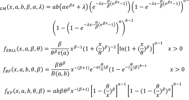
1.12, 1.71, 2.17, 1.17, 5.08, 2.48, 1.18, 3.51, 2.17, 1.69,1.25, 4.38, 1.84, 0.39, 3.68, 2.48, 0.85, 1.61, 2.79, 4.7, 2.03, 1.8, 1.57, 1.08, 2.03, 1.61, 2.12,1.89, 2.88, 2.82, 2.05, 3.65. These data were previously studied by Souza et al. for beta Frechet (BF), exponentiated Frechet (EF) and Frechet distributions. In the following, we shall compare the proposed KGM and its sub-model (GM) with several other three- and four-parameter lifetime distributions, namely: the Zografos-Balakrishnan log-logistic (ZBLL), Kumaraswamy Pareto (KP) and recently the Kumaraswamy Gompertz Makeham (KGM) distribution with corresponding densities:
Where
‡ˆ9 , , , ", , = + A
:
B A1 − : B
‰1 − A1 − : B Š
‹hŒŒ , , ", • =• Ž" 1 + • ]&ln 1 + • ' > 0
hM , , , •, " =l ,"• 4 • 1 − • R?@ > 0
‡= , , , •, " = "• 4 %1 − • ( %1 − 1 − • (
Where , , ", •, , > 0
Table1 gives the descriptive statistics of the data and Table 2 gives the likelihood ratio estimates of the parameters and table 3 gives the values of AIC, BIC, CAIC and HQIC for EGGM, KGM, GM, BF, KP, ZBLL, BF and EF distributions, the corresponding errors(given in parenthesis) and the statistics p •‘ (where p •‘ denotes the log-likelihood function evaluated at the maximum likelihood estimates), Akaike information criterion (AIC), the Bayesian information criterion (BIC), Consistent Akaike information
criterion (CAIC) and Hannan-Quinn information criterion (HQIC). We also construct the Total Time on Test (TTT) plot for the data as well as its empirical density and cumulative density function.
Table 1. Descriptive Statistics on Breaking stress of Carbon fibres.
’“” •– Med. —˜™” •š ’™› œ•žŸ ¡“¡ Skewness
0.390 1.840 2.700 2.6214 3.220 5.560 0.10494 0.36815
Table 2. Likelihood Estimates of Parameters.
’ ¨˜I ©¡Ÿ“—™Ÿ˜¡
U 7
, , •, " 4.15811.6264 4.17571.6094 0.57050.4949 100.0037 0.55113−
« 7
, , , , " 3.2590 (1.8545)
6.7422 (1.18545)
10 (17.4572)
0.22148 (0.74510)
0.130941 (0.71868)
«<
, , •, " 4.69523 (0.502)
236.2335 (149.552)
0.39 -
0.19204 (0.045)
-
¬l--, •¬l--, " 1.5501 (0.104)
1.90903 (0.0093)
3.61259 0.288
- -
l
, , •, " 0.42934 (0.236)
138.0664 (113.552)
34.38484 (21.52)
0.72474 (0.19)
-
7
, , " 10(0.0829)
0.076941
Table 3. Criteria for Comparison.
’ ¨˜I ® ¯°) ±²³ ´²³ HQIC CAIC
U 7 -29.548 69.096 82.122 74.368 69.734
, , •, "
« 7 -141.332 292.664 305.690 297.936 293.599
, , , , "
«< -166.751 339.502 347.318 338.084 339.923
, , •, "
¬l-- -162.913 331.826 339.642 330.408 332.076
, •, "
l -142.866 293.733 304.154 291.842 294.154
, , •, "
7 -149.125 304.25 312.066 307.413 304.50
, , "
Figure 3. The graph of Total Time on Test Plot for the breaking stress of carbon data.
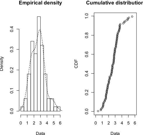
Figure 4. The graph of the Emprical density and the cummulative density of the carbon data.
0.0 0.2 0.4 0.6 0.8 1.0
0
.0
0
.2
0
.4
0
.6
0
.8
1
.0
i/n
T
(i
/n
)
Empirical density
Data
D
e
n
s
it
y
0 1 2 3 4 5 6
0
.0
0
.1
0
.2
0
.3
0
.4
0 1 2 3 4 5 6
0
.0
0
.2
0
.4
0
.6
0
.8
1
.0
Cumulative distribution
Data
C
D
9. Conclusion
Since the EGGM distribution has the lowest, AIC, BIC, CAIC and HQIC values among all other models and its sub-model so it could be chosen as the best sub-model.
References
[1] Bailey RC (1978) Limiting form of the Makeham model and their use for survival analysis of transplant studies. Biometries 34: 725-726.
[2] Bourguignon, M., R. B. Silva, L. M. Zea and G. M. Cordeiro, 2013. The Kumaraswamy Pareto distribution. J. of Stat. Theory and Applications, 12: 129-144.
[3] Cordeiro, G. M., E. M. M. Ortega and Daniel C. C da Cunha. The Exponentiated Generalized Class of Distributions. Journal of Data Science 11(2013), 1-27.
[4] Cordeiro, G. M. and M. de Castro, 2010. A new family of generalized distributions. Journal of Statistical Computation and Simulation, 81: 883-898.
[5] Cordeiro, G. M., et al. The Exponentiated Generalized Class of Distributions. Journal of Data Science 11(2013), 1-27. [6] Chukwu A. U. & Ogunde A. A. (2015), 'On the Beta
Makeham Distribution and its Applications', American Journal of Mathematics and Statistics 2015, 5(3): 137-143. [7] El-Gohary, A. & Al-Otaibi, A. N. (2013), ‘The generalized
Gompertz distribution’, Applied Mathematical Modeling 37(1-2), 13–24.
[8] Finch CE. Chicago: University of Chicago Press; 1990. Longevity. Senescence, and the Genome.
[9] Gupta, R. C., Gupta, P. L. and Gupta, R. D. (1998). Modeling failure time data by Lehmann alternatives. Communications in Statistics - Theory and Methods 27, 887-904.
[10] Gupta, R. D. and Kundu, D. (1999). Generalized exponential distributions. Australian and New Zealand Journal of Statistics 41, 173-188.
[11] Gupta, R. D. and Kundu, D. (2001). Exponentiated exponential family: an alternative to gamma and Weibull. Biometrical Journal 43, 117-130.
[12] Gompertz, B. (1825). "On the Nature of the Function Expressive of the Law of Human Mortality, and on a New Mode of Determining the Value of Life Contingencies. Philosophical Transactions of the Royal Society 115: 513– 585.doi:10.1098/rstl.1825.0026.
[13] Jodra, P. (2009). "A closed form expression for the quantile functions of the Gompertz Makeham distribution". Mathematics and Computers in Simulation 79 (10): 3069– 3075. doi:10.1016/j.matcom.2009.02.002.
[14] Lehmann, E. L. (1953). The power of rank tests. Annals of Mathematical Statistics 24, 23-43. Shahbaz, M. Q., S. Shahbaz and N. S. Butt, 2012. The Kumaraswamy inverse Weibull distribution. Pakistan Journal of Statistics and Operation Research, 8: 479-489.
[15] Makeham, W. M. (1860). "On the Law of Mortality and the Construction of Annuity Tables". J. Inst. Actuaries and Assurance. Mag. 8: 301–310.
[16] Nadarajah, S., and Kotz, S. (2005). The beta exponential distribution. Reliability Engineering and System Safety, 91, 689-697.
[17] Souza, W. M., G. M. Cordeiro and A. B. Simas, 2011. Some results for beta Fréchet distribution. Commun. Statist. Theory-Meth., 40: 798-811.