Numerıcal Approxımatons for Solvıng Partıal Dıfferentıal Equatıons wıth Varıable Coeffıcıents

Published online February 20, 2013 (http://www.sciencepublishinggroup.com/j/acm) doi: 10.11648/j.acm.20130201.13

Numerical approximatons for solving partial differentıal

equations with variable coefficients

Veyis TURUT

Department of Mathematics, Faculty of Arts and Sciences, Batman University, Batman,Turkey

Email address:

[email protected] (V. TURUT)

To cite this article:

Veyis TURUT. Numerıcal Approxımatons for Solvıng Partıal Dıfferentıal Equatıons wıth Varıable Coeffıcıents, Applied and Computa-tional Mathematics. Vol. 2, No. 1, 2013, pp. 19-23. doi: 10.11648/j.acm.20130201.13

Abstract:

In this paper, variational iteration method (VIM) and multivariate padé approximaton (MPA) were compared.

First, partial differential eqaution has been solved and converted to power series by variational iteration method (VIM), then the numerical solution of partial differential eqauation was put into multivariate padé series. Thus the numerical solu-tions ofthe partial differential eqautions were obtained. Numerical solutions of two examples were calculated and results were presented in tables and figures.

Keywords:

Variational Iteration Method (VIM), Multivariate Padé Approximaton (MPA), Partial Differential Equation

(PDE)

1. Introduction

Many powerful numerical and analytical methods have been presented. Among them, the Adomian decomposition method (ADM) [1-4], the variational iteration method (VIM) [5–8], differential transform method (DTM) and multivariate padé approximaton (MPA) [9-15] are relative-ly new approaches providing an anarelative-lytical and numerical approximation to linear and nonlinear problems.

The variational iterational method (VIM) was first pro-posed by He [16,17] and has been succesfully applied to autonomous differential equations, non-linear partial diffe-rential equations, non-linear polycrystalline solids, and other fields.

Multivariate padé approximaton (MPA) has been suc-cessfully applied to solve partial differential equations. Many definitions and theorems have been developed for Multivariate Padé Approximations (MPA) (see [18] for a survey on Multivariate Padé approximation).

2. The Variational Iteration Method

The basic concepts and principles variational iteration method can be seen in [19-22]. Ali and Raslan [25] ob-tained the following iteration formula for general PDE equation (1) by using the basic concepts and principles of variational iteration method:

( , , , ).

t x y z

L u+L u+L u+L u+Nu=g x y z t (1)

where,

L

_t,

L

_x,

L

yand

L

z are linear operators of

t

,

x

,

y

_and

_z

_{, respectively, and}

_N

_{is a non-linear operator.}

According to VIM, the following correction functional can be expressed in

t

-,

x

-,

y

- and

z

-directions, respectively, as follows [25] :

{

}

1

1 0

( , , , ) ( , , , )

( ) ,

n n

t

s n x y z n

u x y z t u x y z t

L u L L L N u g ds

λ

+ = +

+ + + + −

∫

ɶ (2)

{

}

1

2 0

( , , , ) ( , , , )

( ) ,

n n

x

s n t y z n

u x y z t u x y z t

L u L L L N u g d s

λ

+ = +

+ + + + −

∫

ɶ (3)

{

}

1

3 0

( , , , ) ( , , , )

( ) ,

n n

y

s n x t z n

u x y z t u x y z t

L u L L L N u g ds

λ

+ = +

+ + + + −

∫

ɶ (4)

{

}

1

4 0

( , , , ) ( , , , )

( ) .

n n

z

s n x y t n u x y z t u x y z t

L u L L L N u g ds

λ

+ = +

+ + + + −

∫

ɶ (5)

0

n

u

δ

ɶ

=

_{. By this method, first the Lagrange multipliers} are determined λ_i(i=1, 2, 3, 4) which will be identified optimally. The succesive approximations un+1,n≥0, of the solution

u

will be readily obtained by suitable choice of trial function

u

₀ [25]. Consequently , the correction func-tional will give several approximations. Then, one of this approximations was compared with multivariate padé ap-proximation by putting into multivariate padé series .

3. Multivariate Padé Approximation

Consider the bivariate function

f x y

( , )

with Taylor se-ries development

, 0

( , ) i j

ij i j f x y c x y

∞

=

=

∑

(6)

around the origin[24]. We know that a solution of unva-riate Padé approximation problem for

0

( ) i

i i

f x c x

∞

=

=

∑

(7)

is given by

1

0 0 0

1 1

1

( )

m m m n

i i n i

i i i

i i i

m m m n

m n m n m

c x x c x x c x

c c c

p x

c c c

− − = = = + + − + + − =

∑

∑

⋯

∑

⋯ ⋮ ⋮ ⋱ ⋮ ⋯ (8) and 1 1 1 1 ( ) n

m m m n

m n m n m

x x

c c c

q x

c c c

+ + − + + − = ⋯ ⋯ ⋮ ⋮ ⋱ ⋮ ⋯ (9)

Let us now multiply jth row in

p x

( )

and

q x

( )

by

1

j m

x+ − (j=2,...,n+1) _{and afterwards divide} j_{th column in}

( )

p x

and

q x

( )

by j 1

x

− (j=2,...,n+1). This results in a multiplication of numerator and denominator by mn

x

.

Having done so, we get

1

0 0 0

1 1 1 1 1 1 1 1 1 1 1 1 ( )

1 1 1

( )

m m m n

i i i

i i i

i i i

m m m n

m m m n

m n m n m

m n m n m

m m m n

m m m n

m n m n m

m n m n m

c x c x c x

c x c x c x

c x c x c x

p x q x

c x c x c x

c x c x c x

− − = = = + + − + + − + + − + + − + + − + + − + + − + + − =

∑

∑

⋯

∑

⋯ ⋮ ⋮ ⋱ ⋮ ⋯ ⋯ ⋯ ⋮ ⋮ ⋱ ⋮ ⋯ (10)

if (D=detDm n, ≠0).

This quotent of determinants can also immediately be

written down for a bivariate function f x y( , ). The sum

0 k i i i c x =

∑

shall be replaced

k

th partial sum of the Taylor

se-ries development of

f x y

( , )

and the expression k k

c x by

an expression that contains all the terms of degree

k

in ( , )

f x y . Here a bivariate term i j ij

c x y _{is said to be of degree}

i

+

j

. If we define

1

0 0 0

1 1

1 ( , )

m m m n

i j i j i j

ij ij ij

i j i j i j

i j i j i j

ij ij ij

i j m i jm i jm n

i j i j i j

ij ij ij

i jm n i jm n i jm

c x y c x y c x y

c x y c x y c x y

p x y

c x y c x y c x y

− − + = + = + = + = + + = + = + − + = + + = + − + = = ∑ ∑ ∑ ∑ ∑ ∑ ∑ ∑ ∑ ⋯ ⋯ ⋮ ⋮ ⋱ ⋮ ⋯ (11) and 1 1 1

1 1 1

( , )

i j i j i j

ij i j ij

i jm i jm i jm n

i j i j i j

ij ij ij

i j m n i jm n i jm

c x y c x y c x y q x y

c x y c x y c x y

+ = + + = + = + − + = + + = + − + = = ∑ ∑ ∑ ∑ ∑ ∑ ⋯ ⋯ ⋮ ⋮ ⋱ ⋮ ⋯ (12)

Then it is easy to see that ( , )p x y and ( , )q x y are of the form

( , )

( , )

m n m

i j i j i j m n

m n n

i j i j i j m n

p x y a x y

q x y b x y

+ + = + + = = =

∑

∑

(13)

We know that p x y( , ) _and q x y( , ) _{are called Padé}

equa-tions[24]. So the multivariate Padé approximant of order

( , )m n _for f x y( , ) _{is defined as}

,

( , )

( , )

( , )

m n

p x y

r x y

q x y

= (14)

4. Applications and Results

In this section, the two methods VIM and MPA wil be illustrated by two examples. All the results are calculated by using software mapple.

Example 4.1.

Consider the one-dimensional heat equation with varia-ble coefficients

2

( , ) ( , ) 0,

2

t xx

x

u x t − u x t = (15)

and the initial condition 2

( , 0)

u x =x . The variational ite-rational schema of equation (15) has the form[25]

2 1 0 ( , ) ( , ) ( ( , )) ( ( , )) , 2 t

n n n s n xx

x

u + x t u x t λ u x s u x s ds

 

= +  − 

 

∫

ɶ ₍₁₆₎

where n≥0 and u x t0( , )=x2. This yields the stationary

1+λ_{s t=} =0_, λ'_{( )s} =_0.

(17)

Hence, the Lagrange multiplier is

1.

λ = − (18)

Substituting this value of the Lagrange multiplier into the functional (16) gives the iteration formula[25]

2

1

0

( , ) ( , ) ( ( , )) ( ( , )) .

2 t

n n n s n xx

x

u₊ x t =u x t − u x s − u x s ds

 

∫

(19)

Ali and Raslan obtained [25] the folowing succesive ap-proximations, starting with an initial approximation:

2

0( , ) ( , 0)

u x t =u x =x

and using the iteration formula (19),

2 1( , ) (1 ) ,

u x t = +t x

2 2

2( , ) (1 ) ,

2! t u x t = + +t x

2 3

2

3( , ) (1 ) ,

2! 3!

t t

u x t = + + +t x

2 3 4

2

4( , ) (1 ) ,

2! 3! 4!

t t t

u x t = + + + +t x

2 3 4 5

2

5( , ) (1 ) ,

2! 3! 4! 5!

t t t t

u x t = + +t + + + x

2 3 4 5 6

2

6( , ) (1 ) .

2! 3! 4! 5! 6!

t t t t t

u x t = + + + + + +t x (20)

The exact solution is given as ( , ) t 2

u x t =e x in [28]. Now let us calculate the approximate solution of Eq.(20) for

6

m= and n=2 by using Multivariate Padé approximation. To obtain Multivariate Padé equations of Eq.(20) for

6

m

=

and n=2, we use Eqs.(11) and (12). By using Eqs.(11) and (12) We obtain,

2 2 2 2 2 3 2 4 2 2 2 2 2 3 2 2 2 2

2 5 2 4 2 3

2 6 2 5 2 4

8 4 3 2 6

1 1 1 1 1 1

2 6 24 2 6 2

1 1 1

( , )

120 24 6

1 1 1

720 120 24

( 12 72 240 360) 1036800

x x t x t x t x t x x t x t x t x x t x t

p x t x t x t x t

x t x t x t

t t t t t x

+ + + + + + + + +

=

+ + + + =

and

2 5 2 4 2 3

2 6 2 5 2 4

8 2 4

1 1 1

1 1 1

( , )

120 24 6

1 1 1

720 120 24

(30 10 )

86400

q x t x t x t x t

x t x t x t

t t t x

= =

− +

So the Multivariate Padé approximation of order (6, 2)

for eq.(20), that is

4 3 2 2

6,2 2

( 12 72 240 360)

( , )

12(30 10 )

t t t t x

r x t

t t

+ + + +

=

− + (21)

Example 4.2.

Consider the one-dimensional wave equation with varia-ble coefficients

2

( , ) ( , ) 0, 2

tt xx

x

u x t − u x t = (22)

with initial conditions u x( , 0)=x, u xt( , 0)=x2. The cor-rection functional for equation (22) is given as[25]

1

2

0

( , ) ( , )

( ( , ) ) ( ( , ) ) ,

2

n n

t

n s s n x x

u x t u x t

x

u x s u x s d s

λ

+ = +

 

−

 

 

∫

ɶ (23)

where n≥0 and u x t₀( , )= +x tx2. Then, the stationary conditions are

1 0, 1 0, ( ) 0.

s t s t s

λ′ ₌ λ ₌ λ′′

+ = + = = (24)

This in turn gives

s t

λ= − (25)

Substituting this value of the Lagrange multiplier into functional (23) gives the iteration formula [25]

1

2

0

( , ) ( , )

( ) ( ( , )) ( ( , )) .

2

n n

t

n ss n xx

u x t u x t

x

s t u x s u x s ds

+ = +

 

−  − 

 

∫

(26)

Selecting the initial approximation: 2 0( , )

u x t = +x tx , with the itration Formula (26), Ali and Raslan obtained [25] the following succesive approximations

3 2 1

3 5

2 2

3 5 7

2 3

3 5 7 9

2 4

( , ) ( ) ,

3!

( , ) ( ) ,

3! 5!

( , ) ( ) ,

3! 5! 7!

( , ) ( ) ,

3! 5! 7! 9! t

u x t x t x

t t

u x t x t x

t t t

u x t x t x

t t t t

u x t x t x

= + +

= + + +

= + + + +

= + + + + +

(27)

3 5 7 9 11

2

5( , ) ( ) ,

3! 5! 7! 9! 11!

t t t t t

u x t = + + + +x t + + x

The exact solution is given asu x t( , )= +x x2sinht in [28]. Now let us calculate the approximate solution of Eq.(20) for m=11 and n=2 by using Multivariate Padé approxima-tion. To obtain Multivariate Padé equations of Eq.(20) for

11

2 2 3 2 5 2 7 2 9 2 2 3 2 5 2 7 2 2 3 2 5 2 7 2 9

2 11 2 9

2 3 5 7 9

1 1 1 1 1 1 1 1 1 1

6 120 5040 362880 6 120 5040 6 120 5040

1

( , ) 0 0

362880

1 1

0

39916800 362880

( 181440 3144960 136080 2448

19 19

+ + + + + + + + + + + + +

=

=

− + + +

+ +

x x t x t x t x t x t x x t x t x t x t x x t x t x t x t

p x t x t

x t x t

t xt xt xt

xt 5 18

958400 19958400) 262815992119290000

+ xt x t

and

29

2 11 29

2 4 18

1 1 1

1

( , ) 0 0

362880

1 1

0

39916800 362880

( 110 ) 14485008384000

q x t x t

x t x t

t x t

=

= − − +

So the Multivariate Padé approximation of order (11, 2) for eq.(27), that is

2 3

5 7 9

11,2 2

( 181440 3144960

136080 2448 19 19958400 19958400)

( , )

(181440( 110 ))

= −

− + +

+ + + +

−

r

t xt

xt xt xt xt x

x t

t

(28)

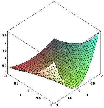
Figure 1. Exact solution of partial differential equation in example 1.

Figure 2. Multivariate Padé approximation for VIM solution of partial differential equation Example 1.

Table 1. Comparison of VIM and MPA for example 1.

x t Exact solution Approximate

solution withMPA

Absolute error of MPA

1.0 1.0 2.718281828 2.718253968 0.000027860

0.9 0.9 1.992278520 1.992268535 5

0 .9 9 8 5×1 0−

0.8 0.8 1.424346194 1.424342992 _{0 .3 2 0 2×1 0}−5

0.7 0.7 0.9867388264 0.9867379342 0.8922 10× −6

0.6 0.6 0.6559627680 0.6559625616 _{0 .2 0 6 4 1 0×} −6

0.5 0.5 0.4121803178 0.4121802805 7

0.373 10× −

0.4 0.4 0.2386919517 0.2386919470 8

0 . 4 7 × 1 0−

0.3 0.3 0.1214872927 0.1214872923 9

0.4 10× −

0.2 0.2 0.04885611032 0.04885611032 0.0

0.1 0.1 0.01105170918 0.01105170918 0.0

Table 2. Comparison of VIM and MPA for example 2.

x t Exact solution

Approximate solution with-MPA

Absolute error of MPA

-2.0 -2.0 12.50744163 12.50744401 5

0.238 10× −

-1.9 -1.9 9.89806811 9.898069207 5

0.110 10× −

-1.8 -1.8 7.732644693 7.732645177 6

0.484 10× −

-1.7 1.7 5.945876289 5.945876494 6

0.205 10× −

-1.6 -1.6 4.481453960 4.481454042 7

0.82 10× −

-1.5 -1.5 3.290878774 3.290878805 7

0.31 10× −

-1.4 -1.4 2.332430942 2.332430954 7

0.12 10× −

-1.3 -1.3 1.570266319 1.570266322 _{0.3 10×} −8

-1.2 -1.2 0.973624351 0.9736243524 8

0.1 10× −

-1.1 -1.1 0.516133439 0.5161334388 0.0

-1.0 -1.0 0.175201194 0.1752011937 0.0

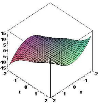
Figure 4. Multivariate Padé approximation for VIM solution of partial differential equation in Example2.

5. Conclusion

The figure which is obtained using MPA and the figure of the exact solution in three-dimensional are shown in figure (1-2) and figure (3-4). As can be seen in table 1, table 2 and figure (1-2), figure (3-4), the approximation solutions with MPA are quite close to exact solutions. It is also observed that MPA is robust and applicable to various types of partial differential equations.

References

[1] G. Adomian, A review of the decomposition method in applied mathematics, J Math Anal Appl (1988), 135: 501– 544.

[2] A. M. Wazwaz, A reliable modification of Adomian decom-position method, Appl Math Comput (1999), 102: 77–86. [3] I. H. Abdel-Halim Hassan, Comparison differential

trans-formation technique with Adomian decomposition method for linear and nonlinear initial value problems, Chaos Soli-tons Fractals (2008), 36: 53–65.

[4] N. Bildik, H. Bayramoglu, The solution of two dimensional nonlinear differential equation by the Adomian decomposi-tion method, Applied Mathematics and Computadecomposi-tion (2005), 163: 519–524.

[5] J. H. He and X. H.Wu, Variational iteration method: new development and applications, Comput Math Appl (2007), 54: 881–894.

[6] J. H. He, Variational iteration method—some recent results and new interpretations, J Comput Appl Math (2007), 207: 3–17.

[7] S. Momani, S. Abuasad, and Z. Odibat, Variational iteration method for solving nonlinear boundary value problems, Appl Math Comput (2006), 183: 1351–1358.

[8] A. Yıldırım and T. Öziş, Solutions of Singular IVPs of Lane-Emden type by the variational iteration method, Non-linear Analysis Ser A: Theory Methods Appl (2009), 70:

2480–2484.

[9] F. Ayaz, Solutions of the System of Differential Equations by Differential Transform Method, Applied Mathematics and Computation (2004) , 147:547-567.

[10] N. Bildik, A. Konuralp, F. Bek, S. Kucukarslan, Solution of different type of the partial differential equation by differen-tial transform method and Adomian’s decomposition me-thod, Appl. Math. Comput. (2006), 172: 551–567.

[11] V. Turut, E. Çelik, M. Yiğider, Multivariate padé approxi-mation for solving partial differential equations (PDE), In-ternational Journal For Numerical Methods In Fluids (2011), 66 (9): 1159–1173.

[12] V. Turut, N. Güzel, Multivariate padé approximation for solving partial differential equations of fractional order, Ab-stract and Applied Analysis (2013), in press.

[13] V. Turut, N. Güzel, Comparing Numerical Methods for Solving Time-Fractional Reaction-Diffusion Equations,

ISRN Mathematical Analysis (2012),

doi:10.5402/2012/737206.

[14] V. Turut,’’ Application of Multivariate padé approximation for partial differential equations’’ , Batman University Jour-nal of Life Sciences (2012), (accepted).

[15] Ph. Guillaume, A. Huard, Multivariate Padé Approximants, Journal of Computational and Applied Mathematics (2000), 121:197-219.

[16] J.H. He, A new approach to nonlinear partial differential equations. Communications in Nonlinear Science and Nu-merical Simulation (1997), 2: 230–235.

[17] J. H. He, Approximate analytical solution for seepage flow with fractional derivatives in porous media. Comput Me-thod Appl Mech Eng (1998), 167: 57–68.

[18] Ph. Guillaume, Nested Multivariate Padé Approximants, J. Comput. Appl. Math. (1997) 82:149-158.

[19] J. H. He, Variational iteration method a kind of nonlinear analytical technique: some examples, Internat J Nonlinear Mech (1999), 34: 699–708.

[20] J. H. He, Variational iteration method for autonomous ordi-nary differential systems, Appl Math Comput (2000), 114 : 115–123.

[21] J. H. He, Some asymptotic methods for strongly nonlinear equations. Int J Mod Phys B (2006), 20: 1141–99.

[22] J. H. He, Wu XH, Construction of solitary solution and compact on-like solution by variational iteration method. Chaos, Solitons & Fractals (2006), 29: 108–13.

[23] J.H. He, Variational principles for some nonlinear partial differential equations with variable coefficients. Chaos, So-litons & Fractals (2004), 19: 847–51.

[24] A. Cuyt, L. Wuytack, Nonlinear Methods in Numerical Analysis, Elsevier Science Publishers B.V. (1987), Amster-dam.