Vol.8 (2018) No. 3
ISSN: 2088-5334
CDM Based Servo State Feedback Controller with Feedback
Linearization for Magnetic Levitation Ball System
Alfian Ma’arif
#, Adha Imam Cahyadi
#, Oyas Wahyunggoro
# #Department of Electrical Engineering and Information Technology, Engineering Faculty, Universitas Gadjah Mada, Yogyakarta, Indonesia
E-mail: [email protected], [email protected], [email protected]
Abstract— This paper explains the design of Servo State Feedback Controller and Feedback Linearization for Magnetic Levitation Ball System (MLBS). The system uses feedback linearization to change the nonlinear model of magnetic levitation ball system to the linear system. Servo state feedback controller controls the position of the ball. An integrator eliminates the steady state error in servo state feedback controller. The parameter of integral gain and state feedback gains is achieved from the concept of Coefficient Diagram Method (CDM). The CDM requires the controllable canonical form, because of that Matrix Transformation is needed. Hence, feedback linearization is applied first to the MLBS then converted to a controllable form by a transformation matrix. The simulation shows the system can follow the desired position and robust from the position disturbance. The uncertainty parameter of mass, inductance, and resistance of MLBS also being investigated in the simulation. Comparing CDM with another method such as Linear Quadratic Regulator (LQR) and Pole Placement, CDM can give better response, that is no overshoot but a quite fast response. The main advantage of CDM is it has a standard parameter to obtain controller’s parameter hence it can avoid trial and error.
Keywords—magnetic levitation ball system; nonlinear; feedback linearization; servo state feedback; coefficient diagram method.
I. INTRODUCTION
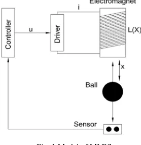
Magnetic Levitation Ball System (MLBS) consists of a mass object that levitates by the force of an electromagnet [1]. The controller is attached to a drive to the electromagnet. The position sensor is also used to measure the distance of the ball from the electromagnet. Fig. 1 represents the model of the MLBS.
Fig. 1 Model of MLBS
MLBS is a modern technology that has high efficiency and frictionless characteristics [2]. This technique is applied
to various systems, such as Suspension [3], Wind Turbine [4], Microbots [5], Bearing [6], Medical [7] and Vehicles [8]. The latest and famous application of MLBS is a Magnetic Levitation (Maglev) train [9].
The other characteristics of MLBS are highly nonlinear, unstable, and difficult to control [10]. Electromagnet coil of MLBS causes the system to be nonlinear. MLBS gives unstable response due to this nonlinearity. Because of that, we need the suitable controller.
Some authors have proposed nonlinear controllers such as Feedback Linearization [11], Sliding Mode Control (SMC) [12], Backstepping [13], High-Gain Observer [14], and Passivity-Based Control [15]. Nonlinear control has advantages in controlling high nonlinear systems such as this MLBS, but it also has disadvantages. SMC has the chattering effect; backstepping is not robust from disturbance, and high-gain observer shows the time response still overshoot. Feedback linearization is sufficient to change nonlinear system to linear system but the parameter gain of linear control that applied still trial and error.
system has to be linearized first, and the result of the linearization must not contain an integrator. Recent author has proposed a PID controller optimized by genetic algorithm as in [17], leading to a better response than conventional PID controller.
Another controller is the fuzzy logic controller (FLC) [20]. FLC also can be applied for controlling MLBS, but it will need more time to design. FLC also needs data from another controller that will be compared to be data for FLC. FLC needs to know the numerical value of the real parameter system model.
Earlier proposed the optimal control in [20], Linear Quadratic Regulator (LQR) is applied by the author to find the state feedback gains parameter correctly. However, the parameter setting of weighting matrix in LQR method still using trial and error.
In this research, the nonlinearity of MLBS will be controlled by feedback linearization which is sufficient to control the nonlinearity. After getting the linear system, servo state feedback controller is chosen to control the position of MLBS. State feedback controller is the most straightforward controller in modern control. The control signal of state feedback is determined by an instantaneous state gain [21]. The main problem of servo state feedback controller is how to choose the effective parameter of integral gain and state feedback gain. These gain change poles of the system that affects the stability and performances of the system. The system will be stable if it has poles on the left side of the imaginary axis. This problem will be solved using Coefficient Diagram Method (CDM).
In CDM, the performance specification is rewritten in a few parameters (stability index and equivalent time constant ) which specify the closed loop transfer function and are related to the controller parameters algebraically in the explicit form [22]. So, trial and error can be avoided by tuning the state feedback gain parameter based on CDM.
As told earlier, the MLBS should change to be linear system and converted into a controllable canonical form to implement servo state feedback controller based on CDM. The controllable form is achieved only by using a transformation matrix.
II. MATERIAL AND METHOD
A. The Concept of CDM
The CDM is an algebraic control design approach with the polynomials, and polynomial matrices are used for system representation and also is a contemporary design [23]. CDM model is based on its stability index and equivalent time constant [22]. The solution process for CDM design will be as follows. The first step is defining the polynomial characteristic of the closed loop transfer function as
) = + + … + + . (1)
Then, it is needed to analyze the performance specifications and design specifications in CDM. Two necessary CDM parameters are the equivalent time constant and the stability index. From the polynomial characteristic ) given in (1), the stability index and equivalent time
constant are respectively described in general term as follows
= , = 1,2, … , − 1), (2)
= . (3)
From the CDM design point of view, only the settling time !"is meaningful because it gives an upper bound of the equivalent time constant as
!"= 2.5~3 . (4)
Thus, the standard form of the equivalent time constant can be described as
= &' (.)~
&'
*. (5)
Besides the equivalent time constant, we need to analyze the stability index. According to [22], the recommended standard form for CDM is
= . .. = *= (= 2, = 2.5. (6)
Another parameter is a stability limit +∗ which defined as follows
+∗=
- +- ; , = ∞. (7)
However, recording of its relation to the stability limit, the condition of stability index can be relaxed as follows
> 1.5 ∗. (8)
The polynomial characteristic is known as the desired characteristic polynomial which is expressed by the coefficient diagram , the equivalent time constant , and stability index . Then should be expressed as
1 ) = 23∑ 5∏
-7 7
89 :
9( ) ; + + 1<, (9)
=∏=7> -= 77
?= . (10)
The next step is assuming controller in the purest possible form and express it in the left polynomial form. Finally, the unknown variables can be solved to get the controller parameters. The adjustment may be needed to satisfy the performance specification.
B. Model of Magnetic Levitation System
D D&E
FG FHI −
FG
FHJ = Υ, (11)
where Υ is the external force acting on the &L generalized coordinate [24].
The kinetic energy and the potential energy of MLBS can be written respectively as following
M =(@ N)O(+
(PNI(, (12)
Q = −PRN, (13)
Where @ N) is a representation of the coil inductance, P is the mass of the ball, N is the position of the ball, and O is the current.
The correlation between coil inductance with the ball position is written as
@ N) = @ + EGSS J = @ + E(TSJ, (14)
Where @ is the electromagnet coil inductance constant, @ is the additional inductance, and N is the reference position. Hence, Lagrangian @ of MLBS is given as
@ = M − Q =(@ N)O(+
(PNI(+ PRN. (15)
From the mechanical point of view, the external force of MLBS is air friction force (U) and later assumed that U = 0 and can be written as
DG D&E
FG FSIJ −
FG
FS= U. (16)
From the electrical point of view, the external force of MLBS can be described as W − OX where W is the applied voltage to MLBS and X is the resistance of the electromagnet coil. Assuming that O is the derivation of , we can get the equation as
DG D&E
FG FYJ −
FG
F = W − OX. (17)
By substituting (15) to (16), we can get the equation as follows
NZ =1[ −1ST + R. (18)
By substituting (14) to (15) and (15) to (17), we can get the equation as follows
D
D& @ N)O − 0) = W − OX (19)
D D&E@ +
(T
SJ O = W − OX (20)
@ DYD&+(TS ODSD&= W − OX (21) DY
D&= \
G −
Y] G + O
(T
G S NI. (22)
State variables that represented MLBS are the position of the ball (N), the velocity of the ball (NI), and the current (O). The input signal of MLBS is the applied voltage (W), so that = W. The output of MLBS is the position of the ball (N). Then we can represent the MLBS in state space representation as follows
^NN( N*
_ = 2NNI
O<, (23)
^NINI( NI*
_ = ` a a a
b N(
−TSc
1S + R
−G]N*+(TG ES SS cJde e e f
+ g 0 0 G
h , (24)
+ = N . (25)
C. Feedback Linearization
The central idea of feedback linearization is to transform a nonlinear system dynamics into (entirely or partly) linear ones so that linear control techniques can be applied. This differs from conventional linearization (i.e., Jacobian linearization) because feedback linearization is achieved by exact state transformation and feedback, rather than by linear approximations of the dynamics. The basic idea of simplifying the form of a system by choosing a different state representation, the choice of coordinate systems. Feedback linearization techniques can be viewed as ways of transforming original system models into equivalent models of a more straightforward form [25].
The nonlinear system has a form of state representation as
iI = U N) + j N) , (26)
+ = ℎ N). (27)
The derivative + is given by
+I =FL S)FS lU N) + R N) m (28)
+I = @[ℎ N) + @nℎ N) . (29)
The system is feedback linearizable if and only if a function ℎ satisfies the partial differential equations and subject to the condition [26] as
@n@[ ℎ N) = 0, = 1,2, … , − 1, (30)
@n@[ ℎ N) ≠ 0. (31)
In other words, the derivation of + must be repeated until it has the dependent variable of the control signal as
+p= @ [
pℎ N) + @
As a consequence, the derivation of + can be repeated until its q&L derivation where q is called the relative degree of the nonlinear system
The output y derivation of MLBS is shown as
+I = N( (33)
+Z = R −TSc
1S (34)
+r = −(T1EScSIc
S J +
(T 1E
ScSI
Sc J. (35)
Substituting (24) to (35), the derivation of + is no longer independent of the control signal as
+r = −sT S Sc 1G St +
(T]Sc
1G S +
(TScS
1S −
(TScu
1S G. (36)
In feedback linearization, there is a change of variables which is notated by i that transform the nonlinear system into an equivalent linear system iI as
i = M N),
iI = vi + w N)l − x N)m. (37)
Remembering the nonlinear system representation before, the component of transformation matrix M N) is described as
M N) = ℎ N), (38)
My N) = @[M N) = @[ℎ N) = 1,2, … , − 1. (39)
Thus, the change of variables i and the new feedback linearized system of MLBS iI are shown as following
i = ℎ N) = N , (40) i(= @[ℎ N) = N(,(41)
i*= @[(ℎ N) = R −1STSc, (42)
And
iI = i(, (43)
iI(= i*, (44)
iI*= −(T1EScSSIcJ +(T1EScSSIc J, (45)
iI*= −sT S S1G Stc+(T]S1G Sc+(TS1ScS −(TS1S Gcu. (46)
The control signal u is written as follows
=G
zG|{ L S)}−@[
pℎ N) + ~•, (47)
where v is the new input designed for the linear system.
Then, by substituting equation (47) to (46), the nonlinearity can be canceled. Then, we can get the linear model of MLBS that can be written as
^iIiI( iI*
_ = ^0 1 00 0 1 0 0 0_ ^
i i( i*
_ + ^00
1_ ~, (48)
+ = i . (49)
D. Servo State Feedback Controller
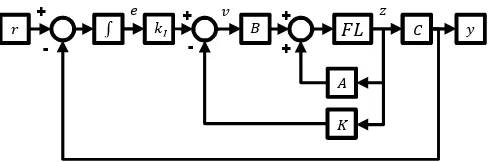
The augmented system (MLBS) is using an integrator to eliminate steady-state error. Diagram block of servo state feedback controller with Feedback Linearization (FL) is shown in Fig. 2.
Fig. 2 Augmented system with servo state feedback controller
The closed-loop state equation from figure 2 can be written as
iI !) = v i !) + w ~ !) + ۥ !), (50)
+ !) = ‚ i !), (51)
where,
v = ƒ v 0−‚ 0„ , w = ƒw0„ , ‚ = l‚ 0m, € = ^⋯0
1_, (52)
i !) = †i !)W !)‡. (53)
To apply state feedback control, the system must fulfill controllability condition as
lw v w v(w v*w m,
Moreover, state controllability condition as
† v−‚ w0 ‡.
The control signal ~ which given to the system can be written as
~ !) = − i !) = −l −ˆYm i !) (54)
= −lˆ ˆ( … ˆ | ˆYm i !) (55)
where are state feedback gains and ˆY is an integral gain. Noting that • !) is a step input, we have • ∞) = • !) = • (constant) for ! > 0. So that the closed loop system (50) with control law (55) is
iI !) = v − w )i !). (56)
+
-~
W + i
-∫ €@
•
v
ˆY w + ‚ +
CDM will design the integral gain and state feedback gains of the control law.
E. Controller Design
The open loop polynomial of the linear MLBS is stated as
‹G ) = |l O − v m|, (57)
= + Π+. . . +Π+ Π. (58)
The equation (50) is not in state variable controllable form, because of that matrix transformation M is needed that can be written as
M = • Ž (59)
where,
• = lw v w v(w … v w m, (60)
Ž = ` a a a b ŒŒ(
⋮ Œ
1 Œ( Œ* ⋮ 1 0
. . . . . . . .
Π1
⋮ 0 0
1 0 ⋮ 0 0de
e e f
. (61)
Defines new state vector by N as
i = MN , (62)
We can get the system in the controllable canonical form as
NI = v•N + w• , (63)
where v• = M v − w )M and w• = M w . The characteristic polynomial from (63) with control signal
= − MN is
‘G ) = | O − v‘+ w•)| (64)
= + ’ˆ“ + Œ ” +. . . +’ˆ“(+ Œ ” + ’ˆ“ + Œ ”, (65) where M is defined as
M = lˆ“ ˆ“( . . . ˆ“ | ˆ“ m. (66)
According to CDM concept, we need to make the desired characteristic polynomial based on stability index and the equivalent time constant. Therefore, we have the coefficients of the desired polynomials to in (9). Finally, from (9), (58), (65) and (59), the gain matrix for the augmented system can be found as
= l − Œ … (− Œ ( | − Œ mM ,
(67)
where = l | ˆYm.
III.RESULTS AND DISCUSSION
The nonlinear model of MLBS uses feedback linearization to change the system to the linear model. Then using the linear control servo state feedback to control the
position of the ball. Finally, servo state feedback is tuned by CDM Concept.
The system is simulated, and the model is generated in SIMULINK MATLAB. Parameters of the simulation are shown in Table 1.
TABLEI
MLBSPARAMETERS
Equilibrium distance (•–—˜) 0.01 P Equilibrium current (•™—˜) 1.6 v
Mass (›) 0.36 ˆR
Acceleration of gravity (œ) 9.8 P/ (
Force constant ( ) 0.00013 ¡P(/v(
Coil resistance (¢) 9 Ω
Coil inductance (¤¥) 0.12 ¦
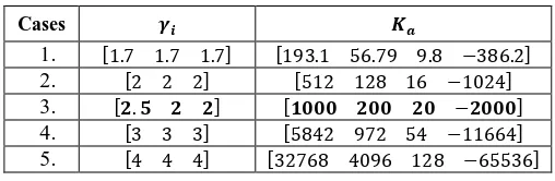
The equivalent time constant is = 0.5. The result of state feedback gains and the integral gain of the augmented system is shown in Table 2. The third value is the CDM standard parameters.
TABLEII
INTEGRAL GAIN VALUE AND SERVO STATE FEEDBACK GAIN
Cases §¥ ¨©
1. l1.7 1.7 1.7m l193.1 56.79 9.8 −386.2m 2. l2 2 2m l512 128 16 −1024m 3. l¬.- ¬ ¬m l–®®® ¬®® ¬® −¬®®®m 4. l3 3 3m l5842 972 54 −11664m 5. l4 4 4m l32768 4096 128 −65536m
CDM gives a good performance and also provides excellent stability of the system, noticed from the values of to . Coefficient diagram which provides stability can be seen in Fig. 3. The most bend curve shows the most stable system. The most bend and stable is case 5 but the standard parameter CDM in case 3 is good enough to make the system stable as shown in Fig. 4.
Fig. 3 The stability of CDM
0 0.5 1 1.5 2 2.5 3 3.5 4 100 101 102 103 104 105
i
ai
1. γγγγi=[1.7 1.7 1.7
2. γγγγi=[2 2 2]
3. γγγγi=[2.5 2 2]
4. γγγγi=[3 3 3]
Fig. 4 Response from the system
Simulations use unit steps • = 1 as the desired position, and the system must follow it. The CDM standard parameters can give a good performance of the position value to reference, without needed to modify the CDM parameters. Comparing with the most bend curve, the standard parameters of CDM have better response on rising time as shown in Fig. 4. It proves that the CDM standard parameter has given good enough performance and stability.
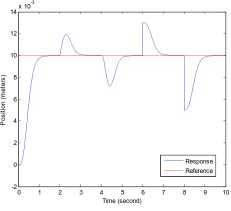
The simulation to investigate the response of the system from disturbance shows in Fig. 5. The simulation uses a standard parameter of CDM (No. 3) as a parameter for servo state feedback gains. The disturbance is given at second, fourth, sixth and eighth seconds. Response from system shows that the controller can make the system stable and follow the desired position.
Fig. 5 Response from disturbance
The simulation about the uncertainty of mass, inductance, and resistance is done to find out how the system performs due to change of the parameter. The simulation is shown in Fig. 6, 7, and 8.
The uncertainty parameter makes the system unstable and affects the position of the steel ball. Object mass uncertainty is given as ±50% and ±90% of the original mass as shown in Fig. 6. The simulation result shows that the uncertainty of mass does not affect the steel ball position too much. The applied controller still can handle the given change of the mass.
Fig. 6 Response from the uncertainty of mass
The uncertainty of inductance is provided between ±25% and ±50% of the original inductance value as shown in Fig. 7. The simulation result indicates that the inductance uncertainty affects the ball position. It also shows that the applied controller still can stabilize the position of its reference point. This is not happening in the real system because the change value of the position exceeds the limit of the position.
Fig. 7 Response to the uncertainty of inductance
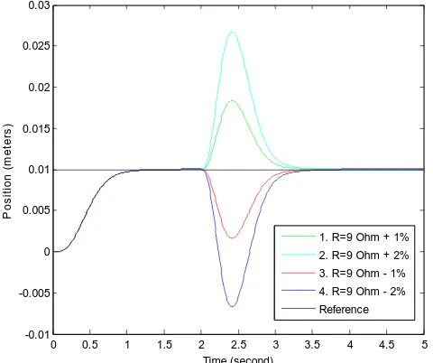
The uncertainty of resistance is given between ±1% and ±2% of the original value of resistance as shown in Fig. 8. The simulation result indicates that the change of the parameter affects the change of object position, even if the
0 0.5 1 1.5 2 2.5 3 3.5 4 4.5 5
0 0.002 0.004 0.006 0.008 0.01 0.012 0.014
Time (second)
P
o
s
it
io
n
(
m
e
te
rs
)
1. γ
i=[1.7 1.7 1.7 2. γ
i=[2 2 2] 3. γ
i=[2.5 2 2] 4. γ
i=[3 3 3] 5. γ
i=[4 4 4] Reference
0 1 2 3 4 5 6 7 8 9 10
-2 0 2 4 6 8 10 12
14x 10
-3
Time (second)
P
o
s
it
io
n
(
m
e
te
rs
)
Response Reference
0 0.5 1 1.5 2 2.5 3
-2 0 2 4 6 8 10 12x 10
-3
Time (second)
P
o
s
it
io
n
(
m
e
te
rs
)
1. m=0,36kg+50% 2. m=0,36kg+90% 3. m=0,36kg-50% 4. m=0,36kg-90% Reference
0 0.5 1 1.5 2 2.5 3 3.5 4 4.5 5
-2 0 2 4 6 8 10 12 14
16x 10
-3
Time (second)
P
o
s
it
io
n
(
m
e
te
rs
)
parameter varies to a slight value. A small value of the parameter uncertainty can give an extreme change of ball position. However, the controller still able to stabilize the system and made the system follows the given reference point as shown in the simulation result. Same as the change of the inductance, the result becomes unreal because it exceeds the position limit.
Fig. 8 Response from the uncertainty of resistance
The simulations that show the comparison of the CDM, LQR, and pole placement method implementation is shown in Fig 9. The comparison is made by showing the system’ performance which is affected by the implementation of the method. Based on that figure, the simulation shows that CDM implementation makes the system performs without giving any overshoot and with quite a fast rise time. By applying pole placement method, the system performs the slowest among all even though there is no overshoot in the response. LQR implementation makes the system performs with an overshoot in response.
The completed response also can be seen in Table III. Based on that table, CDM give the best settling time to stabilize the system and give the smallest overshoot. While LQR gives the fastest rise time but the rise time of CDM is good enough.
TABLEIII
COMPARING CDM WITH LQR AND POLE PLACEMENT
Rise Time (seconds)
Overshoot (%)
Settling Time (seconds)
CDM 0.548 0.016 1.059
LQR 0.501 7.697 1.474
Pole Placement
0.867 0.360 1.505
The difference between CDM, LQR and pole placement method is CDM has a standard parameter and able to minimalize the effort to obtain controller parameter. By using LQR, we still need to determine weighting matrix and also it does not have standard weighting matrix. It is same with pole placement method that needs to determine the pole location. If the pole is too far from the y-axis, then it will
have significant control signal even though the system performs well and stable. However, if it is too close to the y-axis, then it will give bad system’s response.
Fig. 9 Comparing CDM, LQR, and Pole Placement
IV.CONCLUSION
The simulation of Coefficient Diagram Method (CDM) based on Servo State Feedback Controller with Feedback Linearization for Magnetic Levitation Ball System (MLBS) has been done. Feedback linearization can transform the nonlinear model of MLBS to the equivalent linear system so that the linear controller can be applied. The linear servo state feedback controller can be used to control object position. CDM also can be used to get servo state feedback gain or parameter tuning. The implementation of CDM standard parameter can make the object gets the reference point with a good value of rising time and settling time, and also no overshoot performance is obtained. This parameter also gives excellent stability of the system to respond to the disturbances. Comparing CDM with another method such as LQR and pole placement shows that CDM gives fast rise time and no overshoot in system performance. While LQR gives overshoot in the system response and Pole Placement gives a slow response.
The change of plant parameter is an issue to design MLBS controller. Feedback linearization cannot handle the problem of MLBS parameter change. Adaptive control or nonlinear control can be implemented to this matter.
The choice of parameter is a matter of research. CDM concept can be applied in the tuning of the controller parameter. CDM theory can avoid trial and error process, so parameter tuning becomes more efficient.
ACKNOWLEDGMENT
The author would like to thank the Ministry of Higher Education for providing research grant RISTEKDIKTI No. 1715/UN1/DITLIT/DIT-LIT/LT2018.
0 0.5 1 1.5 2 2.5 3 3.5 4 4.5 5
-0.01 -0.005 0 0.005 0.01 0.015 0.02 0.025 0.03
Time (second)
P
o
s
it
io
n
(
m
e
te
rs
)
1. R=9 Ohm + 1% 2. R=9 Ohm + 2% 3. R=9 Ohm - 1% 4. R=9 Ohm - 2% Reference
0 0.5 1 1.5 2 2.5 3
0 0.002 0.004 0.006 0.008 0.01 0.012
Time (second)
P
o
s
it
io
n
(
m
e
te
rs
)
REFERENCES
[1] A. Nayak and B. Subudhi, “Discrete backstepping control of magnetic levitation system with a nonlinear state estimator,” in 2016
IEEE Annual India Conference (INDICON), 2016, pp. 1–5.
[2] T. Kumar and S. Shimi, “Modeling, simulation and control of single actuator magnetic levitation system,” … (RAECS), 2014 Recent …, no. June, pp. 1–6, 2014.
[3] C. Peng, G. Zhaoyu, and L. Jie, “Study on two feedback linearization control methods for the magnetic suspension system,” in 2015 34th
Chinese Control Conference (CCC), 2015, pp. 1059–1063.
[4] N. Patel and M. N. Uddin, “Design and performance analysis of a magnetically levitated vertical axis wind turbine based axial flux PM generator,” in 2012 7th International Conference on Electrical and
Computer Engineering, 2012, pp. 741–745.
[5] M. Mehrtash and M. B. Khamesee, “Optimal motion control of magnetically levitated microrobot,” in 2010 IEEE International
Conference on Automation Science and Engineering, 2010.
[6] P. V. S. Sobhan, G. V. N. Kumar, and J. Amarnath, “Rotor levitation by Active Magnetic Bearings using Fuzzy Logic Controller,” 2010
Int. Conf. Ind. Electron. Control Robot., pp. 197–201, 2010.
[7] M. Simi, G. Sardi, P. Valdastri, A. Menciassi, and P. Dario, “Magnetic Levitation camera robot for endoscopic surgery,” in 2011
IEEE International Conference on Robotics and Automation, 2011,
pp. 5279–5284.
[8] G. G. Sotelo, R. A. H. de Oliveira, F. S. Costa, D. H. N. Dias, R. de Andrade, and R. M. Stephan, “A Full Scale Superconducting Magnetic Levitation (MagLev) Vehicle Operational Line,” IEEE
Trans. Appl. Supercond., vol. 25, no. 3, pp. 1–5, Jun. 2015.
[9] Jaewon Lim, Chang-Hyun Kim, Jong-Min Lee, Hyung-suk Han, and Doh-Young Park, “Design of magnetic levitation electromagnet for High Speed Maglev train,” in 2013 International Conference on
Electrical Machines and Systems (ICEMS), 2013, pp. 1975–1977.
[10] P. Šuster and A. Jadlovská, “Modeling and Control Design of Magnetic Levitation System,” Appl. Mach. Intell. Informatics (SAMI),
2012 IEEE 10th Int. Symp., pp. 295–299, 2012.
[11] M. Ahsan, N. Masood, and F. Wali, “Control of a magnetic levitation system using non-linear robust design tools,” in 2013 3rd IEEE
International Conference on Computer, Control and Communication (IC4), 2013, pp. 1–6.
[12] M. A. Akram, I. Haider, H.-U.-R. Khalid, and V. Uddin, “Sliding mode control for electromagnetic levitation system based on feedback linearization,” in 2015 Pattern Recognition Association of
South Africa and Robotics and Mechatronics International
Conference (PRASA-RobMech), 2015, pp. 78–82.
[13] Huann-Keng Chiang, Wen-Te Tseng, Chun-Chiang Fang, and Chien-An Chen, “Integral backstepping sliding mode control of a magnetic ball suspension system,” in 2013 IEEE 10th International Conference
on Power Electronics and Drive Systems (PEDS), 2013, pp. 44–49.
[14] A. M. Benomair, A. R. Firdaus, and M. O. Tokhi, “Fuzzy sliding control with non-linear observer for magnetic levitation systems,” in
2016 24th Mediterranean Conference on Control and Automation (MED), 2016, pp. 256–261.
[15] T. Namerikawa and H. Kawano, “A passivity-based approach to wide area stabilization of magnetic suspension systems,” in 2006 American
Control Conference, 2006, p. 6 pp.
[16] S. K. Verma, S. Yadav, and S. K. Nagar, “Optimal fractional order PID controller for magnetic levitation system,” in 2015 39th National
Systems Conference (NSC), 2015, pp. 1–5.
[17] I. Ahmad, M. Shahzad, and P. Palensky, “Optimal PID control of Magnetic Levitation System using Genetic Algorithm,” in 2014 IEEE
International Energy Conference (ENERGYCON), 2014, pp. 1429–
1433.
[18] N. Magaji and J. L. Sumaila, “Fuzzy logic controller for magnetic levitation system,” in 2014 IEEE 6th International Conference on
Adaptive Science & Technology (ICAST), 2014, pp. 1–5.
[19] A. M. Benomair and M. O. Tokhi, “Control of single axis magnetic levitation system using fuzzy logic control,” in 2015 Science and
Information Conference (SAI), 2015, pp. 514–518.
[20] A. M. Benomair, F. A. Bashir, and M. O. Tokhi, “Optimal control based LQR-feedback linearisation for magnetic levitation using improved spiral dynamic algorithm,” in 2015 20th International
Conference on Methods and Models in Automation and Robotics, MMAR 2015, 2015, pp. 558–562.
[21] K. Ogata, Modern control engineering. Prentice-Hall, 2010. [22] S. Manabe, “Coefficient diagram method,” in Proceedings of the
14th IFAC Symposium on Automatic Control in Aerospace, 1998, pp.
199–210.
[23] S. Manabe, “Importance of coefficient diagram in polynomial method,” in 42nd IEEE International Conference on Decision and
Control (IEEE Cat. No.03CH37475), pp. 3489–3494.
[24] R. M. Murray, Z. Li, and S. S. Sastry, A Mathematical Introduction
to Robotic Manipulation, vol. 29. 1994.
[25] J.-J. E. Slotine and W. Li, Applied nonlinear control. Prentice Hall, 1991.