Email: {kaneko, shima} @sie.ics.saitama-u.ac.jp
Abstract—In this paper we present a complex linear prediction analysis method for estimating the formant frequencies of noisy speech. The proposed method effectively utilizes the signal (being the analytic signal) which is ignored in the conventional complex linear prediction analysis to achieve noise reduction. Also, the covariance and forward-backward linear prediction (FBLP) methods are compared, and the FBLP method is deployed for predictive coefficients estimation in the proposed method. Experimental results show that the proposed method yields better performance of formant estimation when compared to some conventional methods in white noise.
Index Terms—LPC, formant, noise reduction, analytic signal
I. INTRODUCTION
Free resonances of the vocal-tract system are called formants. Formants are associated with peaks in the smoothed power spectrum of speech [1]. The peak locations, that is, formant frequencies play a fundamental role in speech synthesis, recognition and compression. For example, formant frequencies serve as an important acoustic feature and offer a phonetic reduction in speech recognition [2] . They are also crucial in the design of some hearing aids [3]. From these reasons, we need accurate formant frequency estimation from the speech signal. Among different formant estimation techniques, linear prediction coding (LPC) based methods have received considerable attention [4] [5] [6].
LPC is the most commonly used technique for speech analysis, which can estimate the spectral envelope of the voiced speech signal by modeling it by a set of parameters closely related to the speech production transfer function. The transfer function of the LPC modeling is expressed by.
( ) ∑
(1)
Being an all-pole filter where G is the gain and are the predictive coefficients.
However, LPC analysis suffers from some drawbacks. One of the most famous ones is that the predictive coefficients can be accurately estimated and the voiced speech signal can also be represented accurately in
Manuscript received November 6, 2013; revised February 8, 2014.
free environment. LPC method, however, becomes very difficult to estimate the predictive coefficients in noisy environment. The accuracy of the method will significantly degrade in the presence of additive noise. On the other hand, complex linear prediction coding (CLPC) has been proposed [7]. CLPC is the method for linear prediction using the complex signal called analytic signal. When performing formant estimation, CLPC shows results better than LPC. Especially, the difference between CLPC and LPC is large in the low frequency region. When analyzing the speech signal corrupted by additive noise, however, the estimation accuracy of CLPC becomes lower than that of LPC. Therefore, noise reduction is required to maintain the excellent performance of CLPC in noisy environment.
When implementing CLPC, decimation by a factor of 2 is needed for the analytic signal. In that process, half of the analytic signal is discarded. That is, without using the data being half of the analytic signal, linear prediction is implemented. In this paper, we present a new method of noise reduction by using the lost data when performing the decimation in CLPC. The adverse noise which corrupts the speech signal is assumed to be white noise. We perform an average operation between the two signals generated by the decimation so as to obtain a new enhanced signal. The new enhanced signal could not only emphasis the speech signal but also suppress the effect of the corrupted noise.
The remainder of this paper is organized as follows. Section II explains the proposed method. In Section III, through experiments, we verify the effectiveness of the proposed method by comparing with some other methods. Finally in Section IV, we conclude the paper.
II. PROPOSED METHOD
In this section, we explain the CLPC method briefly and then derive the proposed method. The CLPC method performs linear prediction using the analytic signal obtained by converting the original signal.
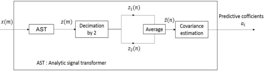
Figure 1. Block diagram of proposed method
( ) ( ) + 𝑗 ( ) (2)
In (2), ( ) and ( ) are related by
( ) ∑∞ ℎ(𝑘)
𝑘=−∞ ( − 𝑘) (3)
where ℎ(𝑘) is the impulse response of the Hilbert transform, which is given by
ℎ(𝑘) {
2 𝜋𝑘𝑠𝑖𝑛
2(𝜋𝑘
2) (𝑘 ≠ 0)
0 (𝑘 0) (4) The analytic signal has an interesting property in the frequency domain. Let the Fourier transform of (𝑛), (𝑛), and (𝑛) be ( ), ( ), and ( ), respectively. Then,
( 𝑤) ( 𝑤) + 𝑗 ( 𝑤) {2 ( 𝑤) (𝜔 > 0)
0 (𝜔 ≤ 0) (5)
Consequently, the analytic signal does not have the negative frequency component, but twice the positive frequency component of the real signal [7].
Let the speech signal be ( ). When the speech signal ( ) is passed through an analytic signal transformer (AST), the corresponding analytic signal ( ) is generated. Then, the analytic signal is decimated by a factor of 2 to expand the spectrum, which is required for the CLPC to obtain an accurate estimation result [7] [8]. Here two signals, (𝑛) and 2(𝑛), are generated. ( ) ,
(𝑛)and 2(𝑛) are related by
(𝑛) (2 ) (6)
2(𝑛) (2 + 1) (7)
where it is noticed that n and m are positive integers such as n = 0,1,2…and m = 0,1,2…. The conventional CLPC method [9] uses only the signal 2(𝑛) to estimate the
predictive coefficients However, the proposed method uses a new analytic signal ̂(𝑛) generated by averaging (𝑛) and 2(𝑛) . The new analytic signal can be
expressed by
̂(𝑛) (𝑛)+ 2(𝑛)
2 (8)
̂(𝑛) (2𝑚)+ 2(2𝑚+ )
2 (9)
The analytic signal (𝑛) is almost similar to 2(𝑛)
because the delay between the signals (𝑛) and 2(𝑛) is
only , where fs is the sampling frequency. This
suggests that ̂(𝑛) results in
̂(𝑛) (𝑛)+ 2(𝑛)
2 (10)
̂(𝑛) ≈ 2(𝑛) (11)
In the proposed method we utilize ̂(𝑛) instead of
2(𝑛).
In the presence of noise ( ), the observed speech signal is given by
𝑦( ) ( ) + ( ) (12)
where ( ) is assumed to white noise with zero mean and variance 2. The analytic signal of the noisy speech 𝑦( ) can be expressed by
𝑦( ) ( ) + 𝑣( ) (13)
where z(m) and 𝑣( ) are the analytic signals of clean
speech and white noise, respectively. Based on the decimation by a factor of 2, the noisy analytic signal
𝑦( ) is divided into
𝑦 (𝑛) (𝑛) + 𝑣 (𝑛) (14)
𝑦2(𝑛) 2(𝑛) + 𝑣2(𝑛) (15)
where 𝑣 (𝑛) and 𝑣2(𝑛) are white noise with zero mean and variance 2, respectively, which are uncorrelated each other. Even in noisy environment, the conventional CLPC method utilizes the 𝑣2(𝑛) to estimate the prediction coefficients . However, in this case, the conventional CLPC method can not reduce the effect of the adverse noise. In this paper, we produce the new analytic signal ̂𝑦(𝑛) to estimate the predictive
coefficients, and set out to reduce the noise effect. The new analytic signal ̂𝑦(𝑛) is expressed by
̂𝑦(𝑛) (𝑛)+ 2(𝑛)+ 2𝑣 (𝑛)+ 𝑣2(𝑛) (16)
̂𝑦(𝑛) ≈ 2(𝑛) + 𝑣 (𝑛)+ 2 𝑣2(𝑛) (17)
As mentioned above, 𝑣 (𝑛) and 𝑣2(𝑛) are uncorrelated white noise with zero mean and variance 2.
The variance of the noise component 𝑣 (𝑛)+ 𝑣2(𝑛)
2 in (17)
In this paper, based on the new analytic signal ̂𝑦(𝑛),
we utilize the Forward-Backward Linear Prediction (FBLP) method [9] [10], being a developed version of the covariance method, to estimate the predictive coefficients. As we know, compared with the autocorrelation method, the covariance method can estimate more accurate prediction coefficients, while it cannot ensure the stability of the resulting all-pole filter. However, it is not necessary to ensure the stability of the all-pole filter in estimating the formant frequencies. In addition, for the complex linear prediction analysis, the target signal is decimated by a factor of 2 from the original signal. This means that the number of the target signal samples becomes half. In this case, the FBLP approach is more effective than the conventional autocorrelation method based approach in [7] to estimate the predictive coefficients from the signal with less length.
In the next session, we verity the effectiveness of the FBLP in a short length signal and the superior performance of the proposed method.
TABLE I. EXPERIMENTAL PARAMETER SPECIFICATION
Sampling frequency 12kHz Analysis window Hamming
LPC order 12
Additive noise White
TABLE II.AEVALUES FOR SYNTHETIC VOWEL /O/
synthetic vowel FBLP(256) FBLP(128) Covariance(256) Covariance(128)
20dB F1 F2 F3
0.0232 0.0232 0.0224 0.0235 0.0172 0.0192 0.0177 0.0262 0.0053 0.0053 0.0026 0.0031
15dB F1 F2 F3
0.0511 0.0511 0.0511 0.0520 0.0378 0.0378 0.0378 0.0396 0.0065 0.0065 0.0065 0.0079
10dB F1 F2 F3
0.1085 0.1085 0.1023 0.1433 0.0606 0.0606 0.0684 0.0696 0.0128 0.0142 0.0121 0.0175
III. EXPERIMENTS
A. Covariance and FBLP Methods for LPC
At first, we investigated the use of the FBLP and covariance methods instead of the autocorrelation method. Only real valued linear prediction, which is not complex-valued linear prediction, was conducted. A synthetic vowel /o/1was generated and used for the experiment. For
1
The synthetic vowel /o/ was generated from an impulsive sequence excitation through the transfer function in (1) with the following parameters: G = 0.134, =0.134, 2 =0.97789, =-1.48396,
=1.78023, =-0.71707, =-0.73514, =0.76348, =-0.12135,
samples with 50% overlap. For each noise level, 100 individual trials to generate white noise were conducted and the calculation of (19) was averaged. In Table II, the evaluated AE is shown for the performance comparison between the FBLP and covariance methods at SNR=20dB, SNR=15dB and SNR=10dB. It is observed that the FBLP method can keep the estimation accuracy when the speech signal is short. Table II suggests that the FBLP method can be extended to a complex-valued version and the complex FBLP method is suitable for complex linear prediction analysis in the proposed method.
B. Results Using Synthetic and Real Vowels
We investigated the performance of the proposed method with the complex FBLP using the synthetic vowel /o/ and five real natural vowels. We compared experimentally the performance of the proposed method with that of the CLPC [7] and INCM [11] in white noise environment. INCM is an iterative noise compensated method, in which the estimation of noise power is computed by using a simplified noise power spectrum estimator proposed by Martin [12].
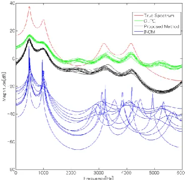
Figure 2. LPC spectra for synthetic vowel /o/ corrupted by white noise at SNR=10dB
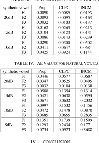
For each noise level, 100 individual trials to generate white noise were conducted again, and the calculation of (19) was averaged. In Table III, for the synthesized vowel /o/ the evaluated AE is shown at SNR=20dB, SNR=15dB and SNR=10dB. It is observed that the proposed method is able to provide reduced AE at any SNR. It should be noticed here that comparing the column of the proposed method in Table III with that of the FBLP method with
256 samples in Table II, the proposed method with the complex FBLP provides more accurate formant frequency estimation with reduced AE values. Fig. 2 shows LPC spectra for the synthetic vowel /o/ corrupted by white noise at SNR=10dB. LPC spectra of the proposed method are most similar to the true spectrum. INCM can not estimate the F3 well.
Next, we investigated in natural vowels /a/, /i/, /u/ ,/e/ and /o/. In the experiment of natural vowels, the true frequency (𝑖) was defined as the estimate of formant frequencies obtained by each method in noise free environment. The evaluated AE values of formant frequencies are shown in Table IV. Table IV shows that the formant estimation accuracy of the proposed method is significant and holds the best performance regardless to SNR. Especially, the estimates of F1 by the proposed method provide high accuracy.
From Tables III and IV, it is commonly observed that the proposed method behaves more robustly against noise in lower SNR conditions.
TABLE III. AEVALUES FOR SYNTHETIC VOWEL /O/
synthetic vowel Prop CLPC INCM
20dB F1 F2 F3 0.0090 0.0093 0.0032 0.0089 0.0095 0.0103 0.0193 0.0163 0.0137 15dB F1 F2 F3 0.0162 0.0104 0.0086 0.0265 0.0123 0.0143 0.0213 0.0131 0.0239 10dB F1 F2 F3 0.0290 0.0411 0.0425 0.0300 0.0647 0.0924 0.0502 0.0684 0.1144
TABLE IV. AEVALUES FOR NATURAL VOWELS
synthetic vowel Prop CLPC INCM
20dB F1 F2 F3 0.0446 0.0347 0.0032 0.0577 0.0525 0.0104 0.0687 0.0495 0.0138 15dB F1 F2 F3 0.0588 0.0421 0.0671 0.1354 0.0638 0.0632 0.1314 0.0595 0.2032 10dB F1 F2 F3 0.0997 0.0472 0.0685 0.1532 0.1478 0.0655 0.1456 0.0870 0.2835 5dB F1 F2 F3 0.1351 0.1293 0.0754 0.1739 0.2434 0.0923 0.1509 0.1771 0.3688 IV. CONCLUSION
In this paper, we have presented a new CLPC analysis method, in which the signal which is ignored in the conventional CLPC analysis is effectively utilized to achieve noise reduction. We investigated the performance of the proposed method using synthetic and natural vowels. As a result, the formant estimation accuracy of the proposed method is significant and holds the best performance in comparing with that of the conventional methods regardless to SNR.
APPENDIX A ANALYSIS OF THE ANALYTIC SIGNAL
In this Appendix, the new analytic signal (18) is discussed more.
The speech signal ( ) is considered as a
combination of multiple sine waves. In the same way, the analytic signals (𝑛) and 2(𝑛) also have the same
characteristics. The analytic signals (𝑛) and 2(𝑛) can
be expressed by the equations belows respectively.
(𝑛) ∑∞ 𝑐𝑜𝑠
= (2𝜋𝑖 (2 ) + 𝜃) (20)
2(𝑛) ∑∞ = 𝑐𝑜𝑠(2𝜋𝑖 (2 + 1) + 𝜃) (21)
where f0 = is the fundamental frequency, T0 is thepitch
period. The analytic signal ̂(𝑛) used by the proposed method is generated by averaging (𝑛)and 2(𝑛). The
analyticsignal ̂(𝑛) can be expressed by
̂(𝑛) (𝑛)+ 2(𝑛)
2 (22)
∑∞ 𝑐𝑜𝑠(2𝜋 (2𝑚)+ )+(2𝜋 2 (2𝑚+ )+ )
=
(2𝜋 (2𝑚+ )+ )−(2𝜋 (2𝑚)+ )
2 (23)
∑∞ 𝑐𝑜𝑠( 𝜋 (2𝑚)+2𝜋 2 +2 )
= 𝑐𝑜𝑠2𝜋 2 (24)
∑∞ 𝑐𝑜𝑠2𝜋𝑖
= (2 +2) 𝑐𝑜𝑠𝜋𝑖 (25)
The larger the i is, the closer to 0 the value of the 𝑐𝑜𝑠𝜋𝑖 is. It means that the components of the 𝑐𝑜𝑠𝜋𝑖 can suppressthe spectrum in the high frequency region. The effect ofthe 𝑐𝑜𝑠 is equivalent to play a role of low-pass filter in the frequency domain. In this case, the locations of formants included in the analytic signal ̂(𝑛) do not change. Therefore, (25) suggests that in a noiseless case, the proposed method does not provide a performance degradation.
REFERENCES
[1] L. Deng, A. Acero, and I. Bazzi,“Tracking vocal tract resonances using a quantized nonlinear function embedded in a temporal constraint,” IEEE Trans. Audio Speech Lang. Processing, vol. 14, no. 2, pp. 425-434, 2006.
[2] L. Welling and H. Ney, “Formant estimation for speech recognition,” IEEE Trans. Speech Audio Process, vol. 6, no. 1, pp. 36-48, 1998.
[3] K. Mustafa and I. C. Bruce, “Robust formant tracking for continuous speech with speaker variability,” IEEE Trans. Audio Speech Lang. Processing, vol. 14, no. 2, pp. 435-444, 2006. [4] R. C. Snell and F. Milinazzo, “Formant location from LPC
analysis data,” IEEE Trans. Speech Audio Processing, vol. 1, no. 2, pp. 129-134, 1993.
[5] G. Duncan and M. A. Jack, ”Pole focusing: A new approach to LPC based speech analysis offering superior formant resolution,” in Proc. IEEE ICASSP, 1988, pp. 2256-2259.
[6] S. Mc Candless, “An algorithm for automatic formant extraction using linear prediction spectra,” IEEE Trans. Acoust. Speech, Signal Processing, vol. ASSP-22, pp.135-141, 1974.
[7] T. Shimamura and S. Takahashi, “Complex linear prediction method based on positive frequency domain,” Electronics and Communication in Japan Part 3, vol. 73, no. 9, pp. 68-77, 1990. [8] S. M. Kay, “Maximum entropy spectral estimation using the
analytic signal,” IEEE Trans. Acoust. Speech, Signal Processing, vol. ASSP-26, no. 10, pp. 467-469, 1978.
[9] S. L. Marple, Digital Spectral Analysis with Applications, Prentice Hall, 1987.
[10] S. Haykin, Adaptive Filter Theory, Prentice Hall, 2001.
University. His research interests include noise