Learning Rates for Q-learning
Eyal Even-Dar [email protected]
Yishay Mansour [email protected]
School of Computer Science Tel-Aviv University
Tel-Aviv, 69978, Israel
Editor: Peter Bartlett
Abstract
In this paper we derive convergence rates for Q-learning. We show an interesting relationship between the convergence rate and the learning rate used in Q-learning. For a polynomial learning rate, one which is 1/tωat time t whereω∈(1/2,1), we show that the convergence rate is poly-nomial in 1/(1−γ), whereγis the discount factor. In contrast we show that for a linear learning rate, one which is 1/t at time t, the convergence rate has an exponential dependence on 1/(1−γ). In addition we show a simple example that proves this exponential behavior is inherent for linear learning rates.
Keywords: Reinforcement Learning, Q-Learning, Stochastic Processes, Convergence Bounds, Learning Rates.
1. Introduction
In Reinforcement Learning, an agent wanders in an unknown environment and tries to maximize its long term return by performing actions and receiving rewards. The challenge is to understand how a current action will affect future rewards. A good way to model this task is with Markov Decision Processes (MDP), which have become the dominant approach in Reinforcement Learning (Sutton and Barto, 1998, Bertsekas and Tsitsiklis, 1996).
An MDP includes states (which abstract the environment), actions (which are the available actions to the agent), and for each state-action pair, a distribution of next states (the states reached after performing the action in the given state). In addition there is a reward function that assigns a stochastic reward for each state and action. The return combines a sequence of rewards into a single value that the agent tries to optimize. A discounted return has a parameterγ∈(0,1)where the reward received at step k is discounted byγk.
One of the challenges of Reinforcement Learning is when the MDP is not known, and we can only observe the trajectory of states, actions and rewards generated by the agent wandering in the MDP. There are two basic conceptual approaches to the learning problem. The first is model based, where we first reconstruct a model of the MDP, and then find an optimal policy for the approximate model. The second approach is implicit methods that update the information after each step, and based on this derive an estimate to the optimal policy. The most popular of those methods is Q-learning (Watkins, 1989).
construct the optimal policy. There are various proofs that Q-learning does converge to the optimal Q function, under very mild conditions (Bertsekas and Tsitsiklis, 1996, Tsitsiklis, 1994, Watkins and Dyan, 1992, Littman and Szepesv´ari, 1996, Jaakkola et al., 1994, Borkar and Meyn, 2000). The conditions have to do with the exploration policy and the learning rate. For the exploration one needs to require that each state action be performed infinitely often. The learning rate controls how fast we modify our estimates. One expects to start with a high learning rate, which allows fast changes, and lowers the learning rate as time progresses. The basic conditions are that the sum of the learning rates goes to infinity (so that any value could be reached) and that the sum of the squares of the learning rates is finite (which is required to show that the convergence is with probability one).
We build on the proof technique of Bertsekas and Tsitsiklis (1996), which is based on conver-gence of stochastic iterative algorithms, to derive converconver-gence rates for Q-learning. We study two models of updating in Q-learning. The first is the synchronous model, where all state action pairs are updated simultaneously. The second is the asynchronous model, where at each step we update a single state action pair. We distinguish between two sets of learning rates. The most interesting outcome of our investigation is the relationship between the form of the learning rates and the rate of convergence. A linear learning rate is of the form 1/t at time t, and a polynomial learning rate,
which is of the form 1/tω, whereω∈(1/2,1)is a parameter.
We show for synchronous models that for a polynomial learning rate the convergence rate is polynomial in 1/(1−γ), while for a linear learning rate the convergence rate is exponential in 1/(1−γ). We also describe an MDP that has exponential behavior for a linear learning rate. The lower bound simply shows that if the initial value is one and all the rewards are zero, it takes
O((1/ε)1/(1−γ))updates, using a linear learning rate, until we reach a value ofε.
The different behavior might be explained by the asymptotic behavior of∑tαt, one of the
condi-tions that ensure that Q-learning converges from any initial value. In the case of a linear learning rate we have that∑Tt=1αt =O(ln(T)), whereas using polynomial learning rate it behaves as O(T1−ω).
Therefore, using polynomial learning rate each value can be reached by polynomial number of steps and using linear learning rate each value requires exponential number of steps.
The convergence rate of Q-learning in a batch setting, where many samples are averaged for each update, was analyzed by Kearns and Singh (1999). A batch setting does not have a learning rate and has much of the flavor of model based techniques, since each update is an average of many samples. A run of a batch Q-learning is divided into phases, at the end of each phase an update is made. The update after each phase is reliable since it averages many samples.
The convergence of Q-learning with linear learning rate was studied by Szepesvari (1998) for special MDPs, where the next state distribution is the same for each state. (This setting is much closer to the PAC model, since there is no influence between the action performed and the states reached, and the states are i.i.d distributed). For this model Szepesvari (1998) shows a convergence rate, which is exponential in 1/(1−γ). Beleznay et al. (1999) give an exponential lower bound in the number of the states for undiscounted return.
2. The Model
We define a Markov Decision process (MDP) as follows
probability from state i to state j when performing action a∈U(i)in state i, and RM(s,a) is the
reward received when performing action a in state s.
We assume that RM(s,a)is non-negative and bounded by Rmax, i.e.,∀s,a : 0≤RM(s,a)≤Rmax.
For simplicity we assume that the reward RM(s,a)is deterministic, however all our results apply
when RM(s,a)is stochastic.
A strategy for an MDP assigns, at each time t, for each state s a probability for performing action
a∈U(s), given a history Ft−1={s1,a1,r1,...,st−1,at−1,rt−1}which includes the states, actions and
rewards observed until time t−1. A policy is memory-less strategy, i.e., it depends only on the current state and not on the history. A deterministic policy assigns each state a unique action.
While following a policy πwe perform at time t action at at state st and observe a reward rt
(distributed according to RM(s,a)), and the next state st+1(distributed according to PsMt,st+1(at)). We
combine the sequence of rewards to a single value called the return, and our goal is to maximize the return. In this work we focus on discounted return, which has a parameter γ∈(0,1), and the discounted return of policyπis VMπ=∑∞t=0γtrt, where rt is the reward observed at time t. Since all
the rewards are bounded by Rmaxthe discounted return is bounded by Vmax=R1max−γ.
We define a value function for each state s, under policyπ, as VMπ(s) =E[∑∞i=0riγi], where the
expectation is over a run of policy π starting at state s. We define a state-action value function
QπM(s,a) =RM(s,a) +γ∑s¯PsM,s¯(a)VMπ(s¯), whose value is the return of initially performing action a
at state s and then following policyπ. Sinceγ<1 we can define another parameterβ= (1−γ)/2, which will be useful for stating our results. (Note that asβdecreases Vmaxincreases.)
Letπ∗ be an optimal policy, which maximizes the return from any start state. (It is well known that there exists an optimal strategy, which is a deterministic policy (Puterman., 1994).) This im-plies that for any policyπand any state s we have VMπ∗(s)≥VMπ(s), andπ∗(s) =argmaxa(RM(s,a)+
γ(∑s0PsM,s0(a)maxbQ(s0,b)). The optimal policy is also the only fixed point of the operator,(T Q)(s,a) =
RM(s,a) +γ∑s0Ps,s0(a)maxbQ(s0,b). We use VM∗ and Q∗Mfor Vπ
∗
M and Qπ
∗
M, respectively. We say that
a policyπis anε-approximation of the optimal policy ifkVM∗−VMπk∞≤ε.
For a sequence of state-action pairs let the covering time, denoted by L, be an upper bound on the number of state-action pairs starting from any pair, until all state-action appear in the sequence. Note that the covering time can be a function of both the MDP and the sequence or just of the sequence. Initially we assume that from any start state, within L steps all state-action pairs appear in the sequence. Later, we relax the assumption and assume that with probability at least 12, from any start state in L steps all state-action appear in the sequence. In this paper, the underlying policy generates the sequence of state action pairs.
The Parallel Sampling Model, PS(M), as was introduced by Kearns and Singh (1999). The
PS(M)is an ideal exploration policy. A single call to PS(M)returns for every pair (s,a)the next state s0, distributed according to PsM,s0(a) and a reward r distributed according to RM(s,a). The
advantage of this model is that it allows to ignore the exploration and to focus on the learning. In some sense PS(M)can be viewed as a perfect exploration policy.
Notations: The notation g=Ω˜(f) implies that there are constants c1 and c2 such that g≥ c1f lnc2(f). All the norms k · k, unless otherwise specified, are L∞ norms, i.e., k(x1,...,xn)k=
3. Q-learning
The Q-learning algorithm (Watkins, 1989) estimates the state-action value function (for discounted return) as follows:
Qt+1(s,a) = (1−αt(s,a))Qt(s,a) +αt(s,a)(RM(s,a) +γ max b∈U(s0)Qt(s
0,b)), (1)
where s0 is the state reached from state s when performing action a at time t. Let Ts,a be the set of times, where action a was performed at state s, then αt(s,a) =0 for t ∈/ Ts,a. It is known
that Q-learning converges to Q∗if each state action pair is performed infinitely often and αt(s,a)
satisfies for each(s,a)pair:∑t∞=1αt(s,a) =∞and∑t∞=1αt2(s,a)<∞(Bertsekas and Tsitsiklis, 1996,
Tsitsiklis, 1994, Watkins and Dyan, 1992, Littman and Szepesv´ari, 1996, Jaakkola et al., 1994). Q-learning is an asynchronous process in the sense that it updates a single entry each step. Next we describe two variants of Q-learning, which are used in the proofs. The first algorithm is
synchronous Q-learning, which performs the updates by using the PS(M). Specifically:
∀s,a : Q0(s,a) =C
∀s,a : Qt+1(s,a) = (1−αtω)Qt(s,a) +αtω(RM(s,a) +γ max
b∈U(s¯)Qt(s¯,b)),
where ¯s is the state reached from state s when performing action a and C is some constant. The
learning rate isαtω=(t+11)ω, forω∈(1/2,1]. We distinguish between a linear learning rate, which isω=1, and a polynomial learning rate, which isω∈(12,1).
The asynchronous Q-learning algorithm, is simply regular Q-learning as define in (1), and we add the assumption that the underlying strategy has a covering time of L. The updates are as follows:
∀s,a : Q0(s,a) =C
∀s,a : Qt+1(s,a) = (1−αωt (s,a))Qt(s,a) +αωt (s,a)(RM(s,a) +γ max
b∈U(s¯)Qt(s¯,b))
where ¯s is the state reached from state s when performing action a and C is some constant. Let
#(s,a,t)be one plus the number of times, until time t, that we visited state s and performed action
a. The learning rateαωt (s,a) = [#(s,1a,t)]ω, if t∈Ts,aandαtω(s,a) =0 otherwise. Again,ω=1 is a
linear learning rate, andω∈(12,1)is a polynomial learning rate.
4. Our Main Results
Our main results are upper bounds on the convergence rates of Q-learning algorithms and showing their dependence on the learning rate. The basic case is the synchronous Q-learning. We show that for a polynomial learning rate we have a complexity, which is polynomial in 1/(1−γ) =1/(2β). In contrast, we show that linear learning rate has an exponential dependence on 1/β. Our results exhibit a sharp difference between the two learning rates, although they both converge with probability one. This distinction, which is highly important, can be observed only when we study the convergence rate, rather than convergence in the limit.
which is exponential in 1β. This implies that our upper bounds are tight, and that the gap between the two bounds is real.
We first prove the results for the synchronous Q-learning algorithm, where we update all the entries of the Q function at each time step, i.e., the updates are synchronous. The following theorem derives the bound for polynomial learning rate.
Theorem 2 Let QT be the value of the synchronous Q-learning algorithm using polynomial
learn-ing rate at time T . Then with probability at least 1−δ, we have that||QT−Q∗|| ≤ε, given that
T=Ω
Vmax2 ln(| S| |A|Vmax
δβε )
β2ε2
1 ω + 1 βln Vmax ε 1 1−ω
The above bound is somewhat complicated. To simplify, assume thatωis a constant and con-sider first only its dependence onε. This gives us Ω((ln(1/ε)/ε2)1/ω+ (ln(1/ε))1/(1−ω)), which is optimized whenω approaches one. Considering the dependence only onβ, recall that Vmax=
Rmax/(2β), therefore the complexity is ˜Ω(1/β4/ω+1/β1/(1−ω)) which is optimized forω=4/5.
The following theorem bounds the time for linear learning rate.
Theorem 3 Let QTbe the value of the synchronous Q-learning algorithm using linear learning rate
at time T . Then for any positive constantψwith probability at least 1−δ, we have||QT−Q∗|| ≤ε,
given that
T =Ω
((2+ψ)β1ln(Vmaxε )V
2
maxln(| S| |A|Vmax
δβψε )
(ψβε)2
.
Next we state our results to asynchronous Q-learning. The bounds are similar to those of syn-chronous Q-learning, but have the extra dependency on the covering time L.
Theorem 4 Let QT be the value of the asynchronous Q-learning algorithm using polynomial
learn-ing rate at time T . Then with probability at least 1−δ, we have||QT−Q∗|| ≤ε, given that
T =Ω
L1+3ωVmax2 ln(| S| |A|Vmax
δβε )
β2ε2
1 ω + L βln Vmax ε 1 1−ω
The dependence on the covering time, in the above theorem, isΩ(L2+1/ω+L1/(1−ω)), which is optimized forω≈0.77. For the linear learning rate the dependence is much worse, since it has to be that L≥ |S| · |A|, as is stated in the following theorem.
Theorem 5 Let QT be the value of the asynchronous Q-learning algorithm using linear learning
rate at time T . Then with probability at least 1−δ, for any positive constantψwe have||QT−Q∗|| ≤
ε, given that
T =Ω
(L+ψL+1)β1lnVmaxε V
2
maxln(| S| |A|Vmax
δβεψ )
(ψβε)2
The following theorem shows that a linear learning rate may require an exponential dependence on 1/(2β) =1/(1−γ), thus showing that the gap between linear learning rate and polynomial learning rate is real and does exist for some MDPs.
Theorem 6 There exists a deterministic MDP, M, such that Q-learning with linear learning rate after T =Ω((1ε)11−γ)steps haskQ
T−Q∗Mk>ε.
5. Experiments
In this section we present experiments using two types of MDPs as well as one we call M0, which
is used in the lower bound example from Section 10. The two MDP types are the “random MDP” and “line MDP”. Each type contains n states and two actions for each state.
We generate the “random MDP” as follows: For every state i, action a and state j, we assign a random number ni,j(a)uniformly from[0,1]. The probability of a transition from state i to state
j while performing action a is pi,j(a) =∑ni,j(a)
kni,k(a). The reward R(s,a)is deterministic and chosen at
random uniformly in the interval[0,10].
For the line MDP, all the states are integers and the transition probability from state i to state j is proportional to |i−1j|, where i6=j. The reward distribution is identical to that of the random MDP.
(We implemented the random function using the function rand() in C.)
0.5 0.55 0.6 0.65 0.7 0.75 0.8 0.85 0.9 0.95 1 0
0.1 0.2 0.3 0.4 0.5 0.6 0.7 0.8 0.9
Learning rate
precision
Random MDP
0.5 0.55 0.6 0.65 0.7 0.75 0.8 0.85 0.9 0.95 1 0
0.1 0.2 0.3 0.4 0.5 0.6 0.7 0.8
Learning rate
precision
Line MDP
Figure 1: Example of 100 states MDP (both line and random), where the discount factor isγ=0.7. We ran asynchronous Q-learning using a random exploration policy for 108steps.
one (an exponential lower and upper bound). Second, the experiments suggest an optimal value for ωof approximately 0.85. Our theoretical results derive optimal values of optimalω for different settings of the parameters but most give a similar range. Furthermore, the two types of MDP have similar behavior, which implies that the difference between linear and polynomial learning rates is inherent to many MDPs and not only special cases (as in the lower bound example).
0.6 0.65 0.7 0.75 0.8 0.85 0.9 0.95 1 10−2
10−1 100 101 102
Discount factor
prec
is
ion
Random MDP
0.6 0.65 0.7 0.75 0.8 0.85 0.9 0.95 1 10−2
10−1 100 101 102
Discount factor
prec
is
ion
Line MDP
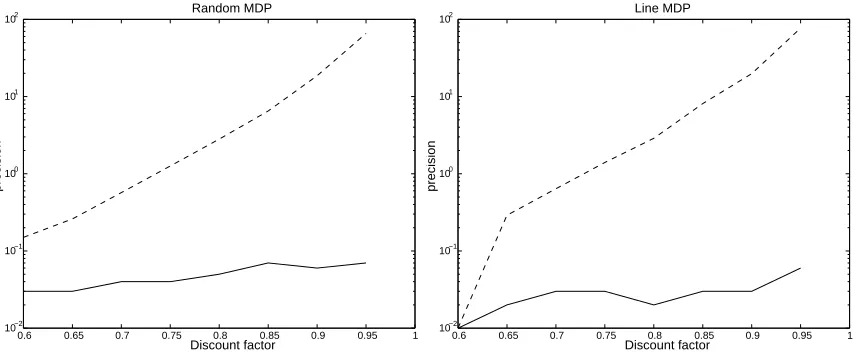
Figure 2: Example of 10 state MDPs (both random and line) using two different learning rates for Q-learning. Both use random exploration policy for 107 steps. The solid line is asynchronous Q-learning usingω=0.7; the dashed line is asynchronous Q-learning using a linear learning rate (ω=1.0).
Figure 2 demonstrates the strong relationship between discount factor,γ, and convergence rate. In this experiment, we again see similar behavior in both MDPs. When the discount factor ap-proaches one, Q-learning using linear learning rate estimation of the Q value becomes unreliable, while Q-learning using learning rate ofω=0.7 remains stable (the error is below 0.1).
Figure 3 compares two different learning ratesω=0.6 andω=0.9 for ten state MDPs (both ran-dom and line) and finds an interesting tradeoff. For low precision levels, the learning rate ofω=0.6 was superior, while for high precision levels the learning rate ofω=0.9 was superior. An explana-tion for this behavior is that the dependence in terms ofεisΩ((ln(1/ε)/ε2)1/ω+ (ln(1/ε))1/(1−ω)), which is optimized as the learning rate approaches one.
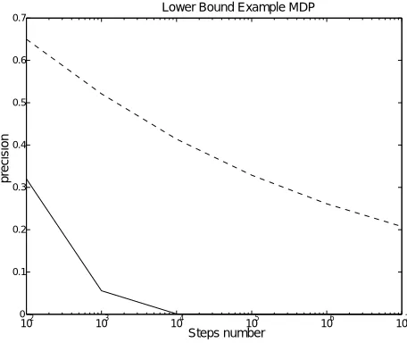
Our last experimental result is M0, the lower bound example from Section 10. Here the
differ-ence between the learning rates is the most significant, as shown in Figure 4.
6. Background from Stochastic Algorithms
102 103 104 105 106 10−3
10−2 10−1 100
101
Steps number
prec
is
ion
Random MDP
102 103 104 105 106 10−3
10−2 10−1 100
101
Steps number
prec
is
ion
Line MDP
Figure 3: Random and Line MPDs (10 states each), where the discount factor is γ=0.9. The dashed line is synchronous Q-learning usingω=0.9 and the the solid line is synchronous Q-learning usingω=0.6.
102 103 104 105 106 107
0 0.1 0.2 0.3 0.4 0.5 0.6 0.7
Steps number
precision
Lower Bound Example MDP
Figure 4: Lower bound example M0, with discount factorγ=0.9. Q-learning ran with two different
learning rates, linear (dashed line) andω=0.65 (solid line).
This section considers a general type of iterative stochastic algorithms, which is computed as follows:
Xt+1(i) = (1−αt(i))Xt(i) +αt(i)((HtXt)(i) +wt(i)), (2)
where wt is a bounded random variable with zero expectation, and each Ht is assumed to belong to
a family
H
of pseudo contraction mappings (See Bertsekas and Tsitsiklis (1996) for details).1. The step sizeαt(i)satisfies (1)∑t∞=0αt(i) =∞, (2)∑∞t=0α2t(i)<∞and (3)αt(i)∈(0,1).
2. There exists a constant A that bounds wt(i)for any history Ft, i.e.,∀t,i : |wt(i)| ≤A.
3. There existsγ∈[0,1)and a vector X∗such that for any X we have||HtX−X∗|| ≤γ||X−X∗||.
The main theorem states that a well-behaved stochastic iterative algorithm converges in the limit.
Theorem 8 [Bertsekas and Tsitsiklis (1996)] Let Xt be the sequence generated by a well-behaved
stochastic iterative algorithm. Then Xtconverges to X∗with probability 1.
The following is an outline of the proof given by Bertsekas and Tsitsiklis (1996). Without loss of generality, assume that X∗=0 andkX0k ≤A. The value of Xt is bounded sincekX0k ≤A and for
any history Ft we havekwtk ≤A; hence, for any t we havekXtk ≤A.
Recall that β= 1−2γ. Let D1=A and Dk+1= (1−β)Dk for k≥1. Clearly the sequence Dk
converges to zero. We prove by induction that for every k there exists some timeτk such that for
any t≥τk we havekXtk ≤Dk. Note that this will guarantee that at time t≥τk for any i the value kXt(i)kis in the interval[−Dk,Dk].
The proof is by induction. Assume that there is such a timeτk and we show that there exists a
timeτk+1such that for t≥τk+1we havekXtk ≤Dk+1. Since Dkconverges to zero this proves that
Xt converges to zero, which equals X∗. For the proof we define for t≥τthe quantity
Wt+1;τ(i) = (1−αt(i))Wt;τ(i) +αt(i)wt(i),
where Wτ;τ(i) =0. The value of Wt;τbounds the contributions of wj(i), j∈[τ,t], to the value of Xt
(starting from timeτ). We also define for t≥τk,
Yt+1;τ(i) = (1−αt(i))Yt;τ(i) +αt(i)γDk
where Yτk;τk =Dk. Notice that Yt;τk is a deterministic process. The following lemma gives the
motivation for the definition of Yt;τk.
Lemma 9 [Bertsekas and Tsitsiklis (1996)] For every i, we have
−Yt;τk(i) +Wt;τk(i)≤Xt(i)≤Yt;τk(i) +Wt;τk(i)
Next we use Lemma 9 to complete the proof of Theorem 8. From the definition of Yt;τ and the
assumption that∑∞t=0αt =∞, it follows that Yt;τ converges toγDk as t goes to infinity. In addition
Wt;τk converges to zero as t goes to infinity. Therefore there exists a time τk+1 such that Yt;τ≤ (γ+β2)Dk, and|Wt;τk| ≤βDk/2. This fact, together with Lemma. 9, yields that for t≥τk+1,
||Xt|| ≤(γ+β)Dk=Dk+1,
7. Applying the Stochastic Theorem to Q-learning
In this section we show that both synchronous and asynchronous Q-learning are well-behaved it-erative stochastic algorithms. The proof is similar in spirit to the proof given by Bertsekas and Tsitsiklis (1996) At the beginning we deal with synchronous Q-learning. First define operator H as
(HQ)(i,a) =
n
∑
j=0
Pi j(a)(R(i,a) +γ max
b∈U(j)Q(j,b))
Rewriting Q-learning with H, we get
Qt+1(i,a) = (1−αt(i,a))Qt(i,a) +αt(i,a)((HQt)(i,a) +wt(i,a)).
Let ¯i is the state reached by performing at time t action a in state i and r(i,s)is the reward observed at time i; then
wt(i,s) =r(i,s) +γ max
b∈U(¯i)Qt(¯i,b)− n
∑
j=0 Pi j(a)
R(i,a) +γ max
b∈U(j)Qt(j,b)
In synchronous Q-learning, H is computed simultaneously on all states actions pairs.
Lemma 10 Synchronous Q-learning is a well-behaved iterative stochastic algorithm.
Proof We know that for any history Ft E[wt(i,a)|Ft] =0 and|wt(i,a)| ≤Vmax. We also know that
for 12<ω≤1 we have that∑αt(s,a) =∞,∑α2t(s,a)<∞andαt(s,a)∈(0,1).
We need only show that H satisfies the contraction property.
|(HQ)(i,a)−(H ¯Q)(i,a)| ≤
n
∑
j=0
Pi j(a)|γ max
b∈U(j)Q(j,b)−γbmax∈U(j)
¯
Q(j,b)|
=
∑
nj=0
Pi j(a)γ| max
b∈U(j)Q(j,b)−bmax∈U(j)
¯
Q(j,b)|
≤
∑
nj=0
Pi j(a)γ max
b∈U(j)|Q(j,b)−
¯
Q(j,b)|
≤ γ
∑
nj=0
Pi j(a)kQ−Q¯k ≤γkQ−Q¯k
Since we update all(i,a)pairs simultaneously, synchronous Q-learning is well-behaved stochas-tic iterative algorithm.
We next show that Theorem 8 can be applied also to asynchronous Q-learning.
Lemma 11 Asynchronous Q-learning, where the input sequence has a finite covering time L, is a well-behaved iterative stochastic algorithm.
Proof We define HQ for every start state i and start time t1of a phase (beginning of the covering time) until the end of the phase (completing the covering time) at time t2, during which all
performed more than once. We consider time t, in which the policy performs action a at state i and
Qtis the vector. We have that
|(HQt)(i,a)−(HQ∗)(i,a)| ≤ n
∑
j=0
Pi j(a)|γ max
b∈U(j)Qt(j,b)−γbmax∈U(j)Q ∗(j,b)|
=
∑
nj=0
Pi j(a)γ| max
b∈U(j)Qt(j,b)−bmax∈U(j)Q ∗(j,b)|
≤
∑
nj=0
Pi j(a)γ max
b∈U(j)|Qt(j,b)−Q ∗(j,b)|
≤
∑
j∈A
Pi j(a)γ max
b∈U(j)|Qt(j,b)−Q ∗(j,b)|
+
∑
j∈B
Pi j(a)γ max
b∈U(j)|Qt(j,b)−Q ∗(j,b)|
≤ γkQt−Q∗k,
where A includes the states for which during (t1,t) all the actions in U(i) were performed, and B=S−A. We conclude thatkQt0−Q∗k ≤ kQt0−1−Q∗k, since we only change at each time a
sin-gle state-action pair, which satisfies|HQt(i,a)−Q∗(i,a)| ≤γ|Qt−Q∗|. We look at the operator H
after performing all state-action pairs, kHQ−Q∗k ≤maxi,a|HQt(i,a)−Q∗(i,a)| ≤γkQt−Q∗k ≤
γkQ−Q∗k.
8. Synchronous Q-learning
In this section we give the proof of Theorems 2 and 3. Our main focus will be the value of rt = kQt−Q∗k, and our aim is to bound the time until rt ≤ε. We use a sequence of values Di, such
that Dk+1= (1−β)Dkand D1=Vmax. As in Section 6, we will consider timesτk such that for any
t≥τkwe have rt ≤Dk. We call the time betweenτkandτk+1the kth iteration. (Note the distinction
between a step of the algorithm and an iteration, which is a sequence of many steps.)
Our proof has two parts. The first (and simple) part is bounding the number of iterations until
Di≤ε. The bound is derived in the following Lemma.
Lemma 12 For m≥1βln(Vmax/ε)we have Dm≤ε.
Proof We have that D1=Vmax and Di = (1−β)Di−1. We want to find the m that satisfies Dm=
Vmax(1−β)m≤ε. By taking a logarithm over both sides of the inequality we get m≥1βln(Vmax/ε).
The second (and much more involved) part is to bound the number of steps in an iteration. We use the following quantities introduced in Section 6. Let Wt+1,τ(s,a) = (1−αtω(s,a))Wt,τ(s,a) +
αω
t (s,a)wt(s,a), where Wτ;τ(s,a) =0 and wt(s,a) =R(s,a) +γ max
b∈U(s0)Qt(s
0,b)−
∑
|S| j=1Ps,j(a)
R(s,a) +γ max
b∈U(j)Qt(j,b)
where s0 is the state reached after performing action a at state s. Let
Yt+1;τk(s,a) = (1−α
ω
t (s,a))Yt;τk(s,a) +α
ω
t (s,a)γDk,
where Yτk;τk(s,a) =Dk. Our first step is to rephrase Lemma 9 for our setting.
Lemma 13 For every state s action a and timeτk, we have
−Yt;τk(s,a) +Wt;τk(s,a)≤Q∗(s,a)−Qt(s,a)≤Yt;τk(s,a) +Wt;τk(s,a)
The above lemma suggests (once again) that in order to bound the error rt one can bound Yt;τk
and Wt;τk separately, and the two bounds imply a bound on rt. We first bound the Yt term, which is
deterministic process, and then we bound the term, Wt;τ, which is stochastic.
8.1 Synchronous Q-learning using a Polynomial Learning Rate
We start with Q-learning using a polynomial learning rate and show that the duration of iteration k, which starts at timeτk and ends at timeτk+1, is bounded byτωk. For synchronous Q-learning with a
polynomial learning rate we defineτk+1=τk+τωk, whereτ1will be specified latter.
Lemma 14 Consider synchronous Q-learning with a polynomial learning rate and assume that for any t≥τkwe have Yt;τk(s,a)≤Dk. Then for any t≥τk+τωk =τk+1we have Yt;τk(s,a)≤Dk(γ+
2
eβ).
Proof Let Yτk;τk(s,a) =γDk+ρτk, whereρτk= (1−γ)Dk. We can now write
Yt+1;τk(s,a) = (1−α
ω
t )Yt;τk(s,a) +αtωγDk=γDk+ (1−αtω)ρt,
whereρt+1=ρt(1−αωt ). We would like to show that after timeτk+1=τk+τωk for any t≥τk+1we
haveρt ≤2eβDk. By definition we can rewriteρt as
ρt = (1−γ)Dk t−τk
∏
l=1
(1−αωl+τk) =2βDk t−τk
∏
l=1
(1−αωl+τk) =2βDk t−τk
∏
l=1
(1− 1
(l+τk)ω),
where the last identity follows from the fact that αωt =1/tω. Since the αtω’s are monotonically decreasing
ρt ≤2βDk(1−
1 τω
k )t−τk.
For t≥τk+τωk we have
ρt ≤2βDk(1−
1 τω
k
)τωk ≤2
eβDk.
Hence, Yt;τk(s,a)≤(γ+2eβ)Dk.
Next we bound the term Wt;τkby(1−
2
e)βDk. The sum of the bounds for Wt;τk(s,a)and Yt;τk(s,a)
would be(γ+β)Dk= (1−β)Dk=Dk+1, as desired.
Definition 15 Let Wt;τk(s,a) = (1−αωt (s,a))Wt−1;τk(s,a) +αωt (s,a)wt(s,a) =∑t
i=τk+1η
k,t
i (s,a)wi(s,a), whereηik,t(s,a) =αiω+τk(s,a)∏ t
j=τk+i+1(1−αωj(s,a))and let Wt;lτk(s,a) =
∑τk+l i=τk+1η
k,t
Note that in the synchronous modelαωt (s,a)andηki,t(s,a)are identical for every state action pair. We also note that Wt;t−τkτk+1(s,a) =Wt;τk(s,a). We have bounded the term Yt;τk, for t=τk+1. This
bound holds for any t≥τk+1, since the sequence Yt;τk is monotonically decreasing. In contrast, the
term Wt;τk is stochastic. Therefore it is not sufficient to bound Wτk+1;τk, but we need to bound Wt;τk
for t≥τk+1. However, it is sufficient to consider t∈[τk+1,τk+2]. The following lemma bounds the
coefficients in that interval.
Lemma 16 For any t∈[τk+1,τk+2]and i∈[τk,t], we haveηki,t=Θ(τ1kω),
Proof Sinceηki,t =αωi+τ
k∏ t
j=τk+i+1(1−αωj),we can divide η k,t
t into two parts, the first oneαωi+τk
and the second one µ=∏tj=τk+i+1(1−αωj). We show that the first one isΘ(τ1ω
k)and the second is
constant. Sinceαωi+τ
k are monotonically decreasing we have for every i∈[τk,τk+2]we haveα
ω τk≤α
ω
i ≤αωτk+2,
thus τ1ω
k ≤α
ω
t ≤(τk+1+1τω k+1)ω ≤
1
(3τωk+τk)ω < 1
4τωk. Next we bound µ. Clearly µ is bounded from above
by 1. Also µ≥∏τk+2
j=τk(1−αj)≥(1−
1 τkω)
3τkω≥ 1
e3. Therefore, we have that for every t∈[τk,τk+2],
ηk,t
i =Θ(τ1kω).
We introduce Azuma’s inequality, which bounds the deviations of a martingale. The use of Azuma’s inequality is mainly needed for the asynchronous case.
Lemma 17 (Azuma 1967) Let X0,X1,...,Xnbe a martingale sequence such that for each 1≤k≤n, |Xk−Xk−1| ≤ck,
where the constant ck may depend on k. Then for all n≥1 and anyε>0
Pr[|Xn−X0|>ε]≤2e
−2∑nε k=1c2k
Next we show that Azuma’s inequality can be applied to Wt;lτk.
Lemma 18 For any t∈[τk+1,τk+2]and 1≤l≤t we have that Wt;lτk(s,a)is a martingale sequence,
which satisfies
|Wt;lτk(s,a)−Wt;l−τk1(s,a)| ≤Θ(Vτmaxω
k )
Proof We first note that Wt;lτk(s,a)is a martingale sequence, since
E[Wt;lτk(s,a)−Wt;l−τk1(s,a)|Fτk+l−1] = E[ηkτ,k+t l(s,a)wτk+l(s,a)|Fτk+l−1]
= ηk,t
τk+lE[wτk+l(s,a)|Fτk+l−1] =0.
By Lemma 16 we have thatηkl,t(s,a) =Θ(1/τωk), thus
|Wt;lτk(s,a)−Wt;l−τk1(s,a)|=ηkτ,k+t l(s,a)|wτk+l(s,a)| ≤Θ(
Vmax
τω
k ).
The following lemma provides a bound for the stochastic error caused by the term Wt;τk by using
Lemma 19 Consider synchronous Q-learning with a polynomial learning rate. With probability at least 1−mδ we have|Wt;τk| ≤(1−
2
e)βDkfor any t∈[τk+1,τk+2], i.e.,
Pr
∀t∈[τk+1,τk+2]: |Wt;τk| ≤(1−
2
e)βDk
≥1− δ
m
given thatτk=Θ((V 2
maxln(Vmax|S| |A|m/(δβDk))
β2D2
k )
1/ω).
Proof By Lemma 18 we can apply Azuma’s inequality to Wt;t−τkτk+1 with ci=Θ( Vmax
τω
k ) (note that
Wt;t−τkτk+1=Wt;τk). Therefore, we derive that
Pr[|Wt;τk(s,a)| ≥ε˜|t∈[τk+1,τk+2]] ≤ 2e
−2˜ε2
∑t
i=τkc2i ≤2e−cτωkε˜2/Vmax2 ,
for some constant c>0. Set ˜δk=2e−cτ
ω
k˜ε2/Vmax2 , which holds forτω
k =Θ(ln(1/δ˜)Vmax2 /ε˜2). Using
the union bound we have,
Pr[∀t∈[τk+1,τk+2]: Wt;τk(s,a)≤ε˜]≤
τk+2
∑
t=τk+1
Pr[Wt;τk(s,a)≤ε˜],
thus taking ˜δk= m(τ δ
k+2−τk+1)|S||A| assures that with probability at least 1−
δ
m the statement hold at
every state-action pair and time t∈[τk+1,τk+2]. As a result we have,
τk=Θ
(Vmax2 ln(|S| |A|mτωk/δ)
˜
ε2 )
1/ω
=Θ
(Vmax2 ln(|S| |A|mVmax/δ˜ε)
˜
ε2 )
1/ω
Setting ˜ε= (1−2/e)βDk gives the desire bound.
We have bounded for each iteration the time needed to achieve the desired precision level with probability 1−mδ. The following lemma provides a bound for the error in all the iterations.
Lemma 20 Consider synchronous Q-learning using a polynomial learning rate. With probability at least 1−δ, for every iteration k∈[1,m]and time t∈[τk+1,τk+2]we have Wt;τk≤(1−
2
e)βDk, i.e.,
Pr
∀k∈[1,m],∀t∈[τk+1,τk+2]: |Wt;τk| ≤(1−
2
e)βDk
≥1−δ,
given thatτ0=Θ((V
2
maxln(Vmax|S| |A|/(δβε))
β2ε2 )1/ω).
Proof From Lemma 19 we know that
Pr
∀t∈[τk+1,τk+2]: |Wt;τk| ≥(1−
2
e)βDk
=Pr
"
∀s,a∀t∈[τk+1,τk+2]:
t
∑
i=τk
wi(s,a)ηki,t≥ε˜
#
≤ δ
Using the union bound we have,
Pr
"
∀s,a∀k≤m,∀t∈[τk+1,τk+2]
t
∑
i=τk
wi(s,a)ηki,t≥ε˜
#
≤
∑
mk=1 Pr
"
∀s,a∀t∈[τk+1,τk+2]
t
∑
i=τk
wi(s,a)ηki,t≥ε˜
#
≤δ
where ˜ε= (1−2e)βDk.
We have bounded both the size of each iteration, as a function of its starting time, and the number of the iterations needed. The following lemma solves the recurrenceτk+1=τk+τωk and
bounds the total time required (which is a special case of Lemma 32).
Lemma 21 Let
ak+1=ak+aωk =a0+
k
∑
i=0 aωi .
For any constantω∈(0,1), ak=O((a10−ω+k)
1
1−ω) =O(ao+k
1 1−ω)
The proof of Theorem 2 follows from Lemma 21, Lemma 20, Lemma 12 and Lemma 14.
8.2 Synchronous Q-learning using a Linear Learning Rate
In this subsection, we derive results for Q-learning with a linear learning rate. The proof is very similar in spirit to the proof of Theorem 2 and we give here analogous lemmas to the ones in Subsection 8.1. First, the number of iterations required for synchronous Q-learning with a linear learning rate is the same as that for a polynomial learning rate. Therefore, we only need to analyze the number of steps in an iteration.
Lemma 22 Consider synchronous Q-learning with a linear learning rate and assume that for any t≥τkwe have Yt;τk(s,a)≤Dk. Then for any t≥(2+ψ)τk=τk+1we have Yt;τk(s,a)≤Dk(γ+
2 2+ψβ) Proof Let Yτk;τk(s,a) =γDk+ρτk, whereρτk= (1−γ)Dk. We can now write
Yt+1;τk(s,a) = (1−αt)Yt;τk(s,a) +αtγDk=γDk+ (1−αt)ρt,
whereρt+1=ρt(1−αt). We would like show that after time(2+ψ)τk=τk+1for any t≥τk+1we
haveρt ≤βDk. By definition we can rewriteρt as,
ρt= (1−γ)Dk t−τk
∏
l=1
(1−αl+τk) =2βDk t−τk
∏
l=1
(1−αl+τk) =2βDk t−τk
∏
l=1
(1− 1
l+τk),
where the last identity follows from the fact thatαt =1/t. Simplifying the expression, and setting
t= (2+ψ)τk, we have
ρt≤2Dkβ
τk
t =
2Dkβ
Hence, Yt;τk(s,a)≤(γ+2+2ψβ)Dk.
The following lemma enables the use of Azuma’s inequality.
Lemma 23 For any t≥τk and 1≤l≤t we have that Wt;lτk(s,a)is a martingale sequence, which
satisfies
|Wt;lτk(s,a)−Wt;l−τk1(s,a)| ≤Vmax t
Proof We first note that Wt;lτk(s,a)is a martingale sequence, since
E[Wt;lτk(s,a)−Wt;l−τk1(s,a)|Fτk+l−1] = E[ηkτ,k+t l(s,a)wτk+l(s,a)|Fτk+l−1]
= ηk,t
τk+lE[wτk+l(s,a)|Fτk+l−1] =0.
For linear learning rate we have thatηkl+,tτ
k(s,a) =1/t, thus
|Wt;lτk(s,a)−Wt;l−τk1(s,a)|=wτk+l(s,a)
t ≤
Vmax
t .
The following Lemma provides a bound for the stochastic term Wt;τk.
Lemma 24 Consider synchronous Q-learning with a linear learning rate. With probability at least
1−mδ, we have|Wt;τk| ≤
ψ
2+ψβDkfor any t∈[τk+1,τk+2]and any positive constantψ, i.e. Pr
∀t∈[τk+1,τk+2]: Wt;τk≤
ψ 2+ψβDk
≥1−δ
m
given thatτk=Θ(V 2
maxln(Vmax|S| |A|m/(ψδβDk))
ψ2β2D2
k )
Proof By Lemma 23 for any t≥τk+1 we can apply Azuma’s inequality to Wt;t−τkτk+1with ci= Vmax i+τk
(note that Wt;t−τkτk+1=Wt;τk). Therefore, we derive that
Pr[|Wt;τk| ≥ε˜|t≥τk+1]≤2e
−2˜ε2
∑t
i=τkc2i =2e− c t2 ˜ε2
(t−τk)V 2max ≤2e−c t ˜ε2 V 2max
for some positive constant c. Using the union bound we get
Pr[∀t∈[τk+1,τk+2]: |Wt;τk| ≥ε˜] ≤ Pr[∀t≥(2+ψ)τk: |Wt;τk| ≥ε˜]
≤
∑
∞t=(2+ψ)τk
Pr[|Wt;τk| ≥ε˜]
≤
∑
∞t=(2+ψ)τk
2e−c
t ˜ε2
V 2max =2e−c
((2+ψ)τk)ε˜2 V 2max
∞
∑
t=0 e−
t ˜ε V 2max
= 2e
−c(2+ψ)τk ˜ε2 V 2max
1−e −˜ε2
V 2max
=Θ(e −c0τk ˜ε2
V 2maxV2 max
˜
where the last equality is due to Taylor expansion and c0 is some positive constant. By setting
δ
m|S| |A| =Θ( e−
c0τk ˜ε2 V 2maxV2
max
˜
ε2 ), which holds forτk=Θ(V 2
maxln(Vmax|S| |A|m/(δε˜))
˜
ε2 ), and ˜ε=
ψ
2+ψβDkassures us
that for every t≥τk+1 (and as a result for any t∈[τk+1,τk+2]) with probability at least 1−mδ the
statement holds at every state-action pair.
We have bounded for each iteration the time needed to achieve the desired precision level with probability 1−mδ. The following lemma provides a bound for the error in all the iterations.
Lemma 25 Consider synchronous Q-learning using a linear learning rate. With probability 1−δ, for every iteration k∈[1,m], time t∈[τk+1,τk+2]and any constantψ>0 we have|Wt;τk| ≤
ψβDk
2+ψ), i.e.,
Pr
∀k∈[1,m],∀t∈[τk+1,τk+2]: |Wt;τk| ≤
ψβDk
2+ψ
≥1−δ,
given thatτ0=Θ(V
2
maxln(Vmax|S| |A|m/(ψδβε))
ψ2β2ε2 ).
Proof From Lemma 19 we know that
Pr
∀t∈[τk+1,τk+2]: |Wt;τk| ≥
ψβDk
2+ψ
≤ δ
m
Using the union bound we have that,
Pr
∀k≤m,∀t∈[τk+1,τk+2]: |Wt;τk| ≥
ψβDk
2+ψ
≤
∑
mk=1 Pr
∀t∈[τk+1,τk+2]: |Wt;τk| ≥
ψβDk
2+ψ
≤δ
The proof of Theorem 5 follows from Lemmas 25 and 22, 12 and the fact that ak+1= (2+
ψ)ak= (2+ψ)ka1.
9. Asynchronous Q-learning
The major difference between synchronous and asynchronous learning is that asynchronous Q-learning updates only one state action pair at each time while synchronous Q-Q-learning updates all state-action pairs at each time unit. This causes two difficulties: the first is that different updates use different values of the Q function in their update. This problem is fairly easy to handle given the machinery introduced. The second, and more basic problem is that each state-action pair should occur enough times for the update to progress. To ensure this, we introduce the notion of covering time, denoted by L. We first extend the analysis of synchronous learning to asynchronous Q-learning, in which each run always has covering time L, which implies that from any start state, in
L steps all state-action pairs are performed. Later we relax the requirement such that the condition
holds only with probability 1/2, and show that with high probability we have a covering time of
distribution of the exploration strategy; it may be the case that at some periods of time certain state-action pairs are more frequent while in other periods different state-state-action pairs are more frequent. In fact, we do not even assume that the sequence of state-action pairs is generated by a strategy—it can be an arbitrary sequence of state-action pairs, along with their reward and next state.
Definition 26 Let n(s,a,t1,t2)be the number of times that the state action pair(s,a)was performed in the time interval[t1,t2].
In this section, we use the same notations as in Section 8 for Dk,τk, Yt;τk and Wt;τk, with a different
set of values forτk. We first give the results for asynchronous Q-learning using polynomial learning
rate (Subsection 9.1); we give a similar proof for linear learning rates in Subsection 9.2.
9.1 Asynchronous Q-learning using a Polynomial Learning Rate
Our main goal is to show that the size of the kth iteration is Lτω
k. The covering time property
guarantees that in Lτω
k steps each pair of state action is performed at leastτωk times. For this reason
we define for asynchronous Q-learning with polynomial learning rate the sequenceτk+1=τk+Lτωk,
whereτ1will be specified later. As in Subsection 8.1 we first bound the value of Yt;τk
Lemma 27 Consider asynchronous Q-learning with a polynomial learning rate and assume that for any t≥τkwe have Yt;τk(s,a)≤Dk. Then for any t≥τk+Lτkω=τk+1we have Yt;τk(s,a)≤D(γ+2eβ)
Proof For each state-action pair(s,a)we are assured that n(s,a,τk,τk+1)≥τωk , since the covering
time is L and the underlying policy has made Lτω
k steps. Using the fact that the Yt;τk(s,a)are
mono-tonically decreasing and deterministic, we can apply the same argument as in the proof of Lemma 14.
The next Lemma bounds the influence of each sample wt(s,a)on Wt;τk(s,a).
Lemma 28 Let ˜wti+τk(s,a) =ηki,t(s,a)wi+τk(s,a)then for any t ∈[τk+1,τk+2]the random variable
˜
wti+τk(s,a)has zero mean and bounded by(L/τk)ωVmax.
Proof Note that by definition wτk+i(s,a)has zero mean and is bounded by Vmaxfor any history and
state-action pair. In a time interval of lengthτ, by definition of the covering time, each state-action pair is performed at leastτ/L times; therefore,ηki,t(s,a)≤(L/τk)ω. Looking at the expectation of
˜
wi+τk(s,a)we observe that
E[w˜ti+τk(s,a)] =E[ηik,t(s,a)wi+τk(s,a)] =η k,t
i (s,a)E[wi+τk(s,a)] =0
Next we prove that it is bounded as well:
|w˜ti+τk(s,a)| = |ηik,t(s,a)wi+τk(s,a)| ≤ |ηk,t
i (s,a)|Vmax ≤ (L/τk)ωVmax
Lemma 29 For any t∈[τk+1,τk+2]and 1≤l≤t we have that Wt;lτk(s,a)is a martingale sequence,
which satisfies
|Wt;lτk(s,a)−Wt;l−τk1(s,a)| ≤(L/τk)ωVmax
Proof We first note that Wt;lτk(s,a)is a martingale sequence, since
E[Wt;lτk(s,a)−Wt;l−τk1(s,a)|Fτk+l−1] = E[w˜tl+τk(s,a)|Fτk+l−1] =0.
By Lemma 28 we have that ˜wtl+τ
k(s,a)is bounded by(L/τk)
ωV
max, thus
|Wt;lτk(s,a)−Wt;l−τk1(s,a)|=w˜tl+τk(s,a)≤(L/τk)ωVmax.
The following Lemma bounds the value of the term Wt;τk.
Lemma 30 Consider asynchronous Q-learning with a polynomial learning rate. With probability at least 1−mδ we have for every state-action pair|Wt;τk(s,a)| ≤(1−e2)βDkfor any t∈[τk+1,τk+2], i.e.
Pr
∀s,a∀t∈[τk+1,τk+2]: |Wt;τk(s,a)| ≤(1−
2
e)βDk
≥1−δ
m
given thatτk=Θ((L 1+3ωV2
maxln(Vmax|S| |A|m/(δβDk))
β2D2
k )
1/ω).
Proof For each state-action pair we look on Wt;lτk(s,a)and note that Wt;τk(s,a) =Wt;t−τkτk+1(s,a). Let
`=n(s,a,τk,t), then for any t ∈[τk+1,τk+2]we have that`≤τk+2−τk≤Θ(L1+ωτωk). By Lemma
29 we can apply Azuma’s inequality to Wt;t−τkτk+1(s,a)with ci= (L/τk)ωVmax. Therefore, we derive
that
Pr[|Wt;τk(s,a)| ≥ε˜|t∈[τk+1,τk+2]] ≤ 2e
−ε˜2 2∑t
i=τk+1,i∈T s,a c
2
i ≤2e−c
˜
ε2τ2ω
k
`V 2maxL2ω
≤ 2e−c
˜
ε2τω
k L1+3ωV 2max,
for some constant c>0. We can set ˜δk=2e−cτ
ω
kε˜2/(L1+3ωVmax)2 , which holds forτω
k =Θ(ln(1/δ˜k)L1+3ωVmax2 /ε˜2).
Using the union bound we have
Pr[∀t∈[τk+1,τk+2]: Wt;τk(s,a)≤ε˜]≤
τk+2
∑
t=τk+1
Pr[Wt;τk(s,a)≤ε˜],
thus taking ˜δk= m(τk+2−τδk+1)|S||A| assures a certainty level of 1−mδ for each state-action pair. As a
result we have
τω
k =Θ(
L1+3ωVmax2 ln(|S| |A|mτωk/δ)
˜
ε2 ) =Θ(
L1+3ωVmax2 ln(|S| |A|mVmax/(δε˜))
˜
ε2 )
Setting ˜ε= (1−2/e)βDk give the desired bound.
Lemma 31 Consider asynchronous Q-learning using a polynomial learning rate. With probability
1−δ, for every iteration k∈[1,m]and time t∈[τk+1,τk+2]we have|Wt;τk(s,a)| ≤(1−
2
e)βDk, i.e.,
Pr
∀k∈[1,m],∀t∈[τk+1,τk+2],∀s,a : |Wt;τk(s,a)| ≤(1−
2
e)βDk
≥1−δ,
given thatτ0=Θ((L
1+3ωV2
maxln(Vmax|S| |A|m/(δβε))
β2ε2 )1/ω).
Proof From Lemma 30 we know that
Pr
∀t∈[τk+1,τk+2]: |Wt;τk| ≥(1−
2
e)βDk
≤ δ
m
Using the union bound we have that
Pr[∀k≤m,∀t∈[τk+1,τk+2] |Wt;τk| ≥ε˜] ≤ m
∑
k=1
Pr[∀t∈[τk+1,τk+2] |Wt;τk| ≥ε˜]≤δ,
where ˜ε= (1−2e)βDk
The following lemma solves the recurrence∑mi=−01Lτωi +τ0and derives the time complexity. Lemma 32 Let
ak+1=ak+Laωk =a0+
k
∑
i=0 Laωi
Then for any constantω∈(0,1), ak=O((a10−ω+Lk) 1
1−ω) =O(a0+ (LK)1−1ω)).
Proof We define the following series
bk+1=
k
∑
i=0
Lbωi +b0
with an initial condition
b0=L
1 1−ω.
We show by induction that bk≤(L(k+1)) 1
1−ω for k≥1. For k=0
b0=L
1
1−ω(0+1)1−1ω ≤L1−1ω
We assume that the induction hypothesis holds for k−1 and prove it for k,
bk=bk−1+Lbωk−1≤(Lk)
1
1−ω+L(Lk)1−ωω ≤L 1
1−ωk1−ωω(k+1)≤(L(k+1)) 1 1−ω
and the claim is proved.
Now we lower bound bk by(L(k+1)/2)1/(1−ω). For k=0
b0=L
1
1−ω ≥(L
2)
Assume that the induction hypothesis holds for k−1 and prove for k,
bk = bk−1+Lbωk−1= (Lk/2)
1
1−ω+L(Lk/2)1−ωω =L1−1ω((k/2)1−1ω+ (k/2)1−ωω)
≥ L1−1ω((k+1)/2)1−1ω.
For a0>L
1
1−ω we can view the series as starting at bk=a0. From the lower bound we know that the start point has movedΘ(a10−ω/L). Therefore we have a total complexity of O((a10−ω+Lk)1−1ω) =
O(a0+ (LK)
1 1−ω)).
The proof of Theorem 4 follows from Lemmas 27, 31,12 and 32. In the following lemma we relax the condition of the covering time.
Lemma 33 Assume that from any start state with probability 1/2 in L steps we perform all state
action pairs. Then with probability 1−δ, from any start state we perform all state action pairs in L log2(1/δ)steps, for a run of length[L log2(1/δ)].
Proof The proof follows from the fact that after k intervals of length L (where k is a natural
num-ber), the probability of not visiting all state action pairs is 2−k. Since we have k= [log2(1/δ)]we get that the probability of failing isδ.
Corollary 34 Assume that from any start state with probability 1/2 in L steps we perform all state
action pairs. Then with probability 1−δ, from any start state we perform all state action pairs in L log(T/δ)steps, for a run of length T .
9.2 Asynchronous Q-learning using a Linear Learning Rate
In this section we consider asynchronous Q-learning with a linear learning rate. Our main goal is to show that the size of the kth iteration is L(1+ψ)τk, for any constantψ>0. The covering time
property guarantees that in(1+ψ)Lτksteps each pair of state action is performed at least(1+ψ)τk
times. The sequence of times in this case isτk+1=τk+ (1+ψ)Lτk, where theτ0 will be defined
latter. We first bound Yt;τk and then bound the stochastic term Wt;τk.
Lemma 35 Consider asynchronous Q-learning with a polynomial learning rate and assume that for any t≥τkwe have Yt;τk(s,a)≤Dk. Then for any t≥τk+(1+ψ)Lτk=τk+1we have Yt;τk(s,a)≤
(γ+ 2
2+ψβ)Dk
Proof For each state-action pair(s,a)we are assured that n(s,a,τk,τk+1)≥(1+ψ)τk, since in an
interval of(1+ψ)Lτksteps each state-action pair is visited at least(1+ψ)τktimes by the definition
of the covering time. Using the fact that the Yt;τk(s,a)are monotonically decreasing and
determin-istic (thus independent), we can apply the same argument as in the proof of Lemma 22.