Linear State-Space Models for Blind Source Separation

Linear State-Space Models for Blind Source Separation

Rasmus Kongsgaard Olsson [email protected]

Lars Kai Hansen [email protected]

Informatics and Mathematical Modelling Technical University of Denmark DK-2800 Lyngby, Denmark

Editor: Aapo Hyv¨arinen

Abstract

We apply a type of generative modelling to the problem of blind source separation in which prior knowledge about the latent source signals, such as time-varying auto-correlation and quasi-periodicity, are incorporated into a linear state-space model. In simulations, we show that in terms of signal-to-error ratio, the sources are inferred more accurately as a result of the inclusion of strong prior knowledge. We explore different schemes of maximum-likelihood optimization for the purpose of learning the model parameters. The Expectation Maximization algorithm, which is often considered the standard optimization method in this context, results in slow convergence when the noise variance is small. In such scenarios, quasi-Newton optimization yields substantial improvements in a range of signal to noise ratios. We analyze the performance of the methods on convolutive mixtures of speech signals.

Keywords: blind source separation, state-space model, independent component analysis,

convo-lutive model, EM, speech modelling

1. Introduction

We are interested in blind source separation (BSS) in which unknown source signals are estimated from noisy mixtures. Real world application of BSS techniques are found in as diverse fields as audio (Yellin and Weinstein, 1996; Parra and Spence, 2000; Anem ¨uller and Kollmeier, 2000), brain imaging and analysis (McKeown et al., 2003), and astrophysics (Cardoso et al., 2002). While most prior work is focused on mixtures that can be characterized as instantaneous, we will here inves-tigate causal convolutive mixtures. The mathematical definitions of these classes of mixtures are given later in this introductory section. Convolutive BSS is relevant in many signal processing ap-plications, where the instantaneous mixture model cannot possibly capture the latent causes of the observations due to different time delays between the sources and sensors. The main problem is the lack of general models and estimation schemes; most current work is highly application specific with the majority focused on applications in separation of speech signals. In this work we will also be concerned with speech signals, however, we will formulate a generative model that may be generalizable to several other application domains.

time-variant statistics. It is well-known that stationary second order statistics, that is, covariances and correlation functions, are not informative enough in the convolutive mixing case.

Our research concerns statistical analysis and generalizations of this approach. We formulate a generative model based on the same statistics as the Parra-Spence model. The benefit of this generative approach is that it allows for estimation of additional noise parameters and injection of well-defined a priori information in a Bayesian sense (Olsson and Hansen, 2005). Furthermore, we propose several algorithms to learn the parameters of the proposed models.

The linear mixing model reads

xt=

L−1

∑

k=0

Akst−k+wt. (1)

At discrete time t, the observation vector, xt, results from the convolution sum of the L time-lagged

mixing matrices Ak and the source vector st. The individual sources, that is, the elements of st, are

assumed to be statistically independent. The observations are corrupted by additive i.i.d. Gaussian

noise, wt. BSS is concerned with estimating st from xt, while Ak is unknown. It is apparent from

(1) that only filtered versions of the elements of st can be retrieved, since the inverse filtering can be

applied to the unknown Ak. As a special case of the filtering ambiguity, the scale and the ordering

of the sources is unidentifiable. The latter is evident from the fact that various permutation applied

simultaneously to the elements of st and the columns of At produce identical mixtures, xt.

Equation (1) collapses to an instantaneous mixture in the case of L=1 for which a variety

of Independent Component Analysis (ICA) methods are available (e.g., Comon, 1994; Bell and Sejnowski, 1995; Hyvarinen et al., 2001). As already mentioned, however, we will treat the class of

convolutive mixtures, that is L>1.

Convolutive Independent Component Analysis (C-ICA) is a class of BSS methods for (1) where the source estimates are produced by computing the ‘unmixing’ transformation that restores statis-tical independence. Often, an inverse linear filter (e.g., FIR) is applied to the observed mixtures. Simplistically, the separation filter is estimated by minimizing the mutual information, or ‘cross’ moments, of the ‘separated’ signals. In many cases non-Gaussian models/higher-order statistics are required, which require a relatively long data series for reliable estimation. This can be executed in the time domain (Lee et al., 1997; Dyrholm and Hansen, 2004), or in the frequency domain (e.g., Parra and Spence, 2000). The transformation to the Fourier domain reduces the matrix convolu-tion of (1) to a matrix product. In effect, the more difficult convolutive problem is decomposed into a number of manageable instantaneous ICA problems that can be solved independently using the mentioned methods. However, frequency domain decomposition suffers from permutation over frequency which is a consequence of the potential different orderings of sources at different fre-quencies. Many authors have explored solutions to the permutation-over-frequency problem that are based on measures of spectral structure (e.g., Anem ¨uller and Kollmeier, 2000), where amplitude correlation across frequency bands is assumed and incorporated in the algorithm.

Olsson and Hansen (2005) added a harmonic excitation component in the source speech model (Brandstein, 1998); this idea is further elaborated and tested here.

Algorithms for the optimization of the likelihood of the linear state-space model are devised and compared, among them the basic EM algorithm, which is used extensively in latent variable models (Moulines et al., 1997). In line with Bermond and Cardoso (1999), the EM-algorithm is shown to exhibit slow convergence in good signal to noise ratios.

It is interesting that the two ‘unconventional’ aspects of our generative model: the non-stationarity of the source signals and their harmonic excitation, do not change the basic quality of the state-space model, namely that exact inference of the sources and exact calculation of the log-likelihood and its gradient are still possible.

The paper is organized as follows: First we introduce the state-space representation of the con-volutive mixing problem and the source models in Section 2, in Section 3 we briefly recapitulate the steps towards exact inference for the source signals, while Section 4 is devoted to a discussion of parameter learning. Sections 5 and 6 present a number of experimental illustrations of the approach on simulated and speech data respectively.

2. Model

The convolutive blind source separation problem is cast as a density estimation task in a latent variable model as was suggested in Pearlmutter and Parra (1997) for the instantaneous ICA problem

p(X|θ) = Z

p(X|S,θ1)p(S|θ2)dS.

Here, the matrices X and S are constructed as the column sets of xt and st for all t. The functional

forms of the conditional likelihood, p(X|S,θ1), and the joint source prior, p(S|θ2), should ideally

be selected to fit the realities of the separation task at hand. The distributions depend on a set of

tunable parameters,θ≡ {θ1,θ2}, which in a blind separation setup is to be learned from the data. In

the present work, p(X|S,θ1)and p(S|θ2)have been restricted to fit into a class of linear state-space

models, for which effective estimation schemes exist (Roweis and Ghahramani, 1999)

st = Fnst−1+Cnut+vt, (2)

xt = Ast+wt. (3)

Equations (2) and (3) describe the state/source and observation spaces, respectively. The parameters of the former are time-varying, indexed by the block index n, while the latter noisy mixing process is stationary. The randomness of the model is enabled by i.i.d. zero mean Gaussian variables,

vt ∼

N

(0,Qn), and wt ∼

N

(0,R) The ‘input’ or ‘control’ signal ut ≡ut(ψn) deterministically

shifts the mean of st depending on parametersψn. Various structures can be imposed on the model

parameters, θ1 ={A,R} and θ2 ={Fn,Cn,Qn,ψn}, in order to create the desired effects. For

equations (2) and (3) to pose as a generative model for the instantaneous mixture of first-order

autoregressive, AR(1), sources it need only be assumed that Fn _{and Q}n _{are diagonal matrices and}

that Cn=0. In this case, A functions as the mixing matrix. In Section 2.1, we generalize to AR(p)

a

!"

# #$ #$% # $ #&

#&$

#&$% #&$

'( )

*

+

+(, -.

!/ !001 !%

!/ "2!(& ! !&%

! &" ! ! & ! %

!&&"3!/ 4 !(& ! &%

54687:9<;4=>@?>A=B7DCFE<=G>

H I J

b

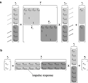
Figure 1: The dynamics of the linear state space model when it has been constrained to describe

a noisy convolutive mixture of P=2 autoregressive (AR) sources. This is achieved by

augmenting the source vector to contain time-lagged signals. In ais shown the

corre-sponding source update, when the order of the AR process is p=4. Inb, the sources are

mixed through filters (L=4) into Q=2 noisy mixtures. Blanks signify zeros.

2.1 Auto-Regressive Source Prior

The AR(p) source prior for source i in frame n is defined as follows,

si,t = p

∑

k=1

f_in_,ksi,t−k+vi,t

where t∈ {1,2, ..,T}, n∈ {1,2, ..,N}and i∈ {1,2, ..,P}. The excitation noise is i.i.d. zero mean

Gaussian: vi,t ∼

N

(0,qni). It is an important point that the convolutive mixture of AR(p) sources

can be contained in the linear state-space model (2) and (3), this is illustrated in Figure 1. The enabling trick, which is standard in time series analysis, is to augment the source vector to include a time history so that it contains L time-lagged samples of all P sources

st =

(s1,t)> (s2,t)> . . . (sP,t)>

>

where the i’th source is represented as

si,t=

si,t si,t−1 . . . si,t−L+1 >

Furthermore, constraints are enforced on the matrices ofθ

Fn = 

   

Fn₁ 0 · · · 0 0 Fn₂ · · · 0

..

. ... . .. ...

0 0 · · · Fn_P      ,

Fn_i =       

f_in_,1 f_in_,2 · · · f_in_,p−1 f_in_,p

1 0 · · · 0 0

0 1 · · · 0 0

..

. ... . .. ... ...

0 0 · · · 1 0

       ,

Qn = 

   

Qn₁ 0 · · · 0 0 Qn₂ · · · 0

..

. ... . .. ...

0 0 · · · Qn_P      ,

(Qn_i)j j0 =

(q2_i)n _{j= j}0₌₁

0 j6=1W

j06=1 ,

Cn = 0,

where Fn_i was defined for p=L. In the interest of the simplicity of the presentation, it is assumed

that Fn_i has L row and columns. We furthermore assume that p≤L; in the case of p<L, zeros

replace the affected (rightmost) coefficients. Hence, the dimensionality of A is Q×(p×P),

A=     

a>₁₁ a>₁₂ .. a>_1P a>₂₁ a>₂₂ .. a>_2P

..

. ... . .. ...

a>_Q1 a>_Q2 .. a>_QP 

   

where ai j = [ai j,1,ai j,2, ..,ai j,L]> can be interpreted as the impulse response of the channel filter

between source i and sensor j. Overall, the model can described can be described as the generative, time-domain equivalent of Parra and Spence (2000).

2.2 Harmonic Source Prior

Many classes of audio signals, such as voiced speech and musical instruments, are approximately piece-wise periodic. By the Fourier theorem, such sequences can be represented well by a harmonic series. In order to account for colored noise residuals and noisy signals in general, a harmonic and noise (HN) model is suggested (McAulay and Quateri, 1986). The below formulation is used

si,t = p

∑

t0₌₁

f_in_,t0si,t−t0+

K

∑

k=1

cn_i,2k−1sin(ωn_0,it) +cn_i,2kcos(ωn_0,it) +vi,t

where ωn_0,i’ is the fundamental frequency of source i in frame n and the Fourier coefficients are

through the definitions

Cn = 

     

(cn

1)> 0 · · · 0

0 0 · · · 0

0 (cn

2)> · · · 0

..

. ... . .. ...

0 0 · · · (cn

P)>



      ,

cn_i =

cn_i,1 cn_i,2 · · · cn_i,2K > , un_t =

(un

1,t)> (un2,t)> . . . (unP,t)>

> ,

where the k’th harmonics of source i in frame n are defined as(un

i,t)2k−1=sin(kωn0,it)and(uni,t)2k=

cos(kωn_0,it), implying the following parameter set for the source mean: ψn=hωn

0,1ωn0,2 . . . ωn0,P

i

. Other parametric mean functions could, of course, be used, for example, a more advanced speech model.

3. Source Inference

In a maximum a posteriori sense, the sources, st, can be optimally reconstructed using the Kalman

filter/smoother (Kalman and Bucy, 1960; Rauch et al., 1965). This is based on the assumption

that the parametersθare known, either a priori or have been estimated as described in Section 4.

While the filter computes the time-marginal moments of the source posterior conditioned on past and present samples, that is,hstip(S|x1:t,θ)and

sts>t

p(S|x1:t,θ), the smoother conditions on samples

from the entire block: hstip(S|x1:T,θ)and

sts>t

p(S|x1:T,θ). For the Kalman filter/smoother to compute

MAP estimates, it is a precondition due that the model is linear and Gaussian. The computational

complexity is

O

(T L3) due to a matrix inversion occurring in the recursive update. Note that the

forward recursion also yields the exact log-likelihood of the parameters given the observations,

L

(θ). A thorough review of linear state-space modelling, estimation and inference from a machine

learning point of view can be found in Roweis and Ghahramani (1999).

4. Learning

The task of learning the parameters of the state-space model from data is approached by

maximum-likelihood estimation, that is, the log-maximum-likelihood function,

L

(θ), is optimized with respect to the

parameters,θ. The log-likelihood is defined as a marginalization over the hidden sources

L

(θ) =log p(X|θ) =log

Z

p(X,S|θ)dS.

A closed-form solution,θ=arg max_θ0

L

(θ0), is not available, hence iterative algorithms that

opti-mize

L

(θ)are employed. In the following sections three such algorithms are presented.

4.1 Expectation Maximization Algorithm

is iterative optimization of a lower bound decomposition of the log-likelihood

L

(θ) ≥

F

(θ,ˆp) =

J

(θ,ˆp)−

R

(ˆp) (4)

where ˆp(S)is any normalized distribution and the following definitions apply

J

(θ,ˆp) = Z

ˆp(S)log p(X,S|θ)dS,

R

(ˆp) = Z

ˆp(S)log ˆp(S)dS.

Jensen’s inequality leads directly to (4). The algorithm alternates between performing Expectation

(E) and Maximization (M) steps, guaranteeing that

L

(θ) does not decrease following an update.

On the E-step, the Kalman smoother is used to compute the marginal moments from the source

posterior, ˆp=p(S|X,θ), see Section 3. The M-step amounts to optimization of

J

(θ,ˆp)with respect

toθ(since this is the only

F

(θ,ˆp)term which depends onθ. Due to the choice of a linear Gaussian

model, closed-form estimators are available for the M-step (see appendix A for derivations). In order to improve on the convergence speed of the basic EM algorithm, the search vector

devised by the M-step update is premultiplied by an adaptive step-sizeη. A simple exponentially

increase of ηfrom 1 was used until a decrease in

L

(θ) was observed at which point ηwas reset

to 1. This speed-up scheme was applied successfully in Salakhutdinov and Roweis (2003). Below

follow the M-step estimators for the AR and HN models. All expectationsh·iare over the source

posterior, p(S|X,θ):

4.1.1 AUTOREGRESSIVEMODEL

For source i in block n:

fn_i,new =

h T+t0(n)

∑

t=2+t0(n)

hsi,t−1s>i,t−1i

i−>h T+t0(n)

∑

t=2+t0(n)

hsi,tsi,t−1i i

,

qn_i,new = 1 T−1

T+t0(n)

∑

t=2+t0(n)

h

hs2_i,ti − fn_i,new

>

hsi,tsi,t−1i i

,

where t0(n) = (n−1)T . Furthermore:

Anew =

hNT

∑

t=1

xthsti>

ihNT

∑

t=1

hst(st)>i

i−1 ,

Rnew = 1 NT

NT

∑

t=1

diag[xt(xt)>−Anewhsti(xt)

>_],

where the diag[·]operator extracts the diagonal elements of the matrix. Following an M-step, the

solution corresponding to ||Ai||=1 ∀i is chosen, where || · || is the Frobenius norm and Ai =

ai1 ai2 · · · aiQ

>

, meaning that A and Qn_{are scaled accordingly.}

4.1.2 HARMONIC ANDNOISEMODEL

The linear source parameters and signals are grouped as

dn_i ≡ (fn

i)> (cni)>

>

, zi≡

(si,t−1)> (ui,t)>

where

fn_i ≡

f_in_,1 f_in_,2 . . . f_in_,p >

, cn_i ≡

ci,1 cni,2 . . . cni,p

> .

It is in general not trivial to maximize

J

(θ,ˆp)with respect toωn_i,0, since several local maxima exist,

for example, at multiples ofωn_i,0 (McAulay and Quateri, 1986). However, simple grid search in a

region provided satisfactory results. For each point in the grid we optimize

J

(θ,ˆp)with respect to

dn_i:

dn_i,new= "

NT

∑

t=2

D

zi,t(zi,t)>

E #−1 NT

∑

t=2 D

zi,t(si,t)>

E .

The estimators of A, R and qn_i are similar to those in the AR model.

4.2 Gradient-based Learning

The derivative of the log-likelihood, dL_d(_θθ), can be computed and used in a quasi-Newton (QN)

optimizer as is demonstrated in Olsson et al. (2006). The computation reuse the analysis of the

M-step. This can be realized by rewriting

L

(θ)as in Salakhutdinov et al. (2003):

d

L

(θ)

dθ =

Z

p(S|X,θ)d log p(X,S|θ)

dθ dS=

d

J

(θ,ˆp)

dθ . (5)

Due to the definition of

J

(θ,ˆp), the desired gradient in (5) can be computed following an E-step

at relatively little effort. Furthermore, the analytic expressions are available from the derivation of the EM algorithm, see appendix A for details. A minor reformulation of the problem is necessary

in order to maintain non-negative variances. Hence, the reformulationsΩ2=R and(φn

i)2=qni are

introduced. Updates are devised forΩandφn_i. The derivatives are

d

L

(θ)

dA = −R

−1_ANT

∑

t=1

D sts>t

E +R−1

N

∑

t=1

xt

D s_t>

E ,

d

L

(θ)

dΩ = Ω

−3NT

∑

t=1

h

xtx>t +A

D stst>

E

A>−2xt

D

s_t>EA>i,

d

L

(θ)

dfn_i =

T+t0(n)

∑

t=2+t0(n)

h

hsi,tsi,t−1i − D

si,t−1s>i,t−1 E

fn_i/qn_ii,

d

L

(θ)

dφn_i = (1−T)/φ

n

i +

φ−3

i

T−1+t0(n)

∑

t=2+t0(n)

hD

si,ts>i,t

E

+ (fn_i)>Dsi,t−1s>i,t−1 E

fn_i −2(fn_i)>Dsi,ts>i,t−1 Ei

.

In order to enforce the unit L2 norm on Ai, a Lagrange multiplier is added to the derivative of A. In

4.3 Stochastic Gradient Learning

Although quasi-Newton algorithms often converge rapidly with a high accuracy, they do not scale well with the number of blocks, N. This is due to the fact that the number of parameters is asymp-totically proportional to N, and therefore the internal inverse Hessian approximation becomes

in-creasingly inaccurate. In order to be able to efficiently learnθ2(A and R) for large N, a stochastic

gradient approach (SGA), (Robbins and Monro, 1951), is employed.

It is adapted here to estimation in block-based state-space models, considering only a single randomly and uniformly sampled block, n, at any given time. The likelihood term corresponding to

block n is

L

(θn₁,θ2), whereθn₁={Fn,Cn,Qn,ψn_{}. The stochastic gradient update to be applied is}

computed at the current optimum with respect toθn₁,

∆θ2 = η

d

L

(θˆn₁,θ2)

dθ2 ,

ˆ θn

1 = arg max

θn

1

L

(θn

1,θ2).

where ˆθn₁is estimated using the EM algorithm. Employing an appropriate ‘cooling’ of the learning

rate, η, is mandatory in order to ensure convergence: one such, devised by Robbins and Monro

(1951), is choosingηproportional to 1_k where k is the iteration number. In our simulations, the SGA

seemed more robust to the initial parameter values than the QN and the EM algorithms.

5. Learning from Synthetic Data

In order to investigate the convergence of the algorithms, AR(2) processes with time-varying pole placement were generated and mixed through randomly generated filters. For each signal frame,

T =200, the poles of the AR processes were constructed so that the amplification, r, was fixed

while the center frequency was drawn uniformly from

U

(π/10,9π/10). The filter length was L=8

and the coefficients of the mixing filters, that is, the ai j of A, were generated from i.i.d. Gaussians

weighted by an exponentially decaying function. Quadratic mixtures with Q=P=2 were used: the

first 2 elements of a12and a21were set to zero to simulate a situation with different channel delays.

All channel filters were normalized to||ai j||2=1. Gaussian i.i.d. noise was added in each channel,

constructing the desired signal to noise ratio.

For evaluation purposes, the signal-to-error ratio (SER) was computed for the inferred sources. The true and estimated sources were mapped to the output by filtering through the direct channel

so that the true source at the output is ˜si,t=aii∗si,t. Similarly defined, the estimated source at the

sensor is ˆsi,t. Permutation ambiguities were resolved prior to evaluating the SER,

SERi=

∑ts˜2i,t

∑t(s˜i,t−sˆi,t)2

.

The EM and QN optimizers were applied to learn the parameters from N=10 frames of samples

with SNR=20dB, r =0.8. The algorithms were restarted 5 times with random initializations,

Ai j∈

N

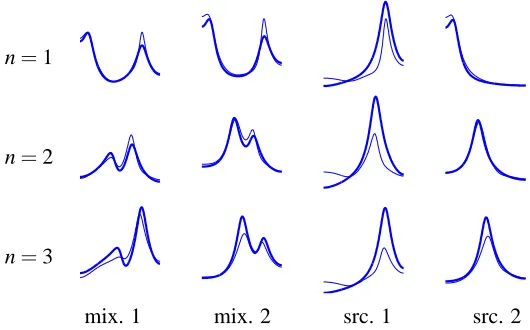
(0,1), the one that yielded the maximal likelihood was selected. Figure 2 shows the results

OLSSON ANDHANSEN 2 4 0 2 4 0 2 4 0 2 4 0 2 4 0 2 4 0 2 4 0 2 4 0 2 4 0 2 4 0 2 4 0 2 4 0 1 2 0 0.5 1 0 0.5 1 0 0.5 1 0 1 2 0 0.5 1 0 0.5 1 0 0.5 1 0 0.5 1 0 0.5 1 0 0.5 1 0 0.5 1 n=1

n=2

n=3

mix. 1 mix. 2 src. 1 src. 2

Figure 2: The true (bold) and estimated models for the first 3 frames of the synthetic data based on the autoregressive model. The amplitude frequency responses of the combined source and channel filters are shown: for source i, this amounts to the frequency response of

the filter, with the scaling and poles ofθ1,i and zeros of the direct channel aii. For the

mixtures, the responses across channels were summed. The EM algorithm provided the estimates.

Estimated Generative MSE FIR

AR 9.1±0.4 9.7±0.4 7.5±0.2

HN 11.8±0.7 13.2±0.4 7.9±0.5

Table 1: The signal-to-error ratio (SER) performance on synthetic data based on the autoregressive (AR) and harmonic-and-noise (HN) source models. Mean and standard deviation of the mean are shown for 1) the EM algorithm applied to the mixtures, 2) inferences from data and the true model, and, 3) the optimal FIR filter separator. The mean SER and the standard

deviation of the mean were calculated from N=10 signal frames, SNR=20dB.

in a supervised fashion was optimized to minimize the squared error between the estimated and

true sources, LFIR=25. Depending on the signal properties, the generative approach, which

re-sults in a time-varying filter, rere-sults in a clear advantage over the time-invariant FIR filter, which has to compromise across the signal’s changing dynamics. As a result, the desired signals are only sub-optimally inferred by methods that apply a constant filter to the mixtures. The performance of the learned model is upper-bounded by that of the generative model, since the maximum likelihood estimator is only unbiased in the limit.

PSfrag replacements

SNR

SER

EM (α=1.2)

QN

EM (α=1.0) EM (α=1.2)

0 10 20 25 30 35 40

0

5 10 15

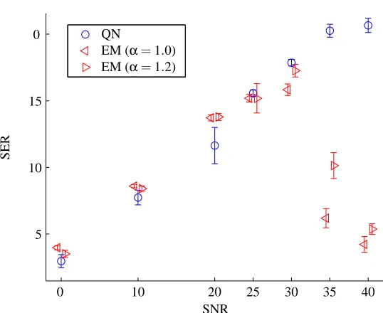
Figure 3: Convergence properties of the EM and QN algorithms as measured on the synthetic data (autoregressive sources). The signal-to-error ratio (SER) was computed in a range of SNR following 300 iterations. As the SNR increases, more accurate estimates are provided by all algorithms, but the number of iterations required increases more dramatically for the EM algorithm. Results are shown for the basic EM algorithm as well as for the step-size adjusted version.

of iterations (imax=300). It should be noted that the time consumption per iteration is similar for the

two algorithms, since a similar number of E-step computations is used (and E-steps all but dominate the cost).

For the purpose of analyzing the HN model, a synthetic data set was generated. The fundamental frequency of the harmonic component was sampled uniformly in a range, see Figure 4, amplitudes

and phases, K=4, were drawn from a Gaussian distribution and subsequently normalized such that

||ci||=1. The parameters of the model were estimated using the EM algorithm on data, which was

constructed as SNR=20dB, HNR=20dB. The fundamental frequency search grid was defined

by 101 evenly spaced points in the generative range. In Figure 4, true and learned parameters are displayed. A close match between the true and estimated harmonics is observed.

In cases when the sources are truly harmonic and noisy, it is expected that the AR model per-forms worse than the HN model. This is due to the fact that a harmonic mean structure is required

for the model to be unbiased. The AR model will compensate by estimating a larger variance, qi,

OLSSON ANDHANSEN

PSfrag replacements

ω0

ˆ_ω0

0.08 0.09 0.1 0.11 0.12 0.08 0.09 0.1 0.11 0.12 300 350 400 250 300 350 400 250 300 350 400 250 300 350 400 250 300 350 400 250 300 350 400 -2 0 2 -2 0 2 -2 0 2 -2 0 2 -2 0 2 -1 0 1

n=1

n=2

n=3

src. 1 src. 2

Figure 4: The true and estimated parameters from synthetic mixtures of harmonic-and-noisy sources as obtained by the EM algorithm. Left: fundamental frequencies in all frames. Right: the waveforms of the true (bold) and estimated harmonic components. For visual-ization purposes, the estimated waveform was shifted by a small offset.

PSfrag replacements HNR (dB) SER (dB) HN (30dB) AR (10dB) AR (20dB) AR (30dB) HN (10dB) HN (20dB) HN (30dB) 0 0.1 0.2 0.3 0.4 0.5 0.6 0.7 0.8 0.9 1

-20 -10 0 10 20 30

0 0.1 0.2 0.3 0.4 0.5 0.6 0.7 0.8 0.9 1 10 15 20 25

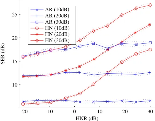
Figure 5: The signal-to-error ratio (SER) performance of the autoregressive (AR) and

harmonic-and-noisy (HN) models for the synthetic data set (N=100) in which the

harmonic-to-noise ratio (HNR) was varied. Results are reported for SNR=10,20,30dB. The results

indicate that the relative advantage of using the correct model (HN) can be significant. The error-bars represent the standard deviation of the mean.

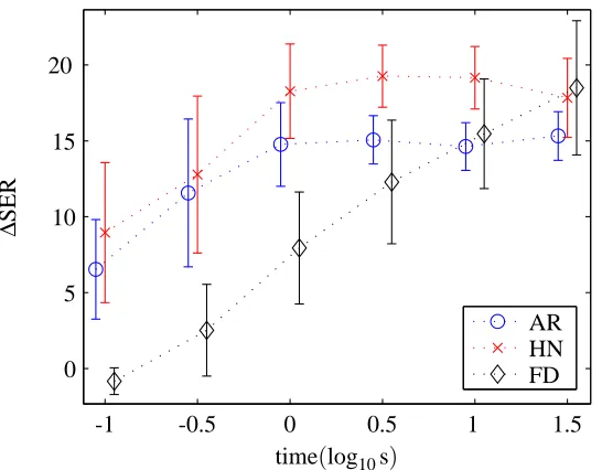
6. Speech Mixtures

LINEARSTATE-SPACEMODELS FORBLINDSOURCESEPARATION

time(log₁₀s)

∆

SER

FD

AR HN FD 0

0.2 0.4 0.6 0.8 1

-1 -0.5 0 0.5 1 1.5

0 0.2 0.4 0.6 0.8 1

0 5 10 15 20

Figure 6: The separation performance (SER) on test mixtures as a function of the training data duration for the autoregressive (AR) and harmonic-and-noisy (HN) priors. Using the stochastic gradient (SG) algorithm, the parameters were estimated from the training data. Subsequently, the learned filters, A, were applied to the test data, reestimating the source model parameters. The noise was constructed at 40dB and assumed known. For ref-erence, a frequency domain (FD) blind source separation algorithm was applied to the data.

we investigate the models based on the autoregressive (AR) and harmonic-and-noisy source (HN) priors and compare with a standard frequency domain method (FD). More specifically, a learning curve was computed in order to illustrate that the inclusion of prior knowledge of speech benefits the separation of the speech sources. In Figure 6 is shown the relationship between the separation performance on test mixtures and the duration of the training data, confirming the hypothesis that the AR and HN models converge faster than the FD method. Furthermore it is seen that the HN model can obtain a larger SER than the AR model.

The mixtures were constructed by filtering speech signals (sampled at 8Hz) through a set of

simulated room impulse responses, that is, ai j, and subsequently adding the filtered signals. The

room impulse responses were constructed by simulating Q=2 speakers and P=2 microphones

in an (ideal) anechoic room, the cartesian coordinates in the horizontal plane given (in m) by

{(1,3),(3,3)} and {(1.75,1),(2.25,1)} for the speakers and microphones, respectively.1. This

corresponds to a maximum distance of 1.25m between the speakers and the microphones, and a set

of room impulse responses that are essentially Kronecker delta functions well represented using a

filter length of L=8.

The SG algorithm was used to fit the model to the mixtures and subsequently infer the source

signals. The speech data, divided into blocks of length T =200, was preprocessed with a standard

pre-emphasis filter, H(z) =1−0.95z−1, and inversely filtered prior to the SER calculations. From

initial conditions (qn_i =1, f_in_,j =0, c_in_,j =0 and ai,j,k normally distributed, variance 0.01, for all

i,j,n,k except a1,1,1=1, a2,2,1=1;ωn_0,i was drawn from a uniform distribution corresponding to

the interval 50−200Hz), the algorithm was allowed imax=500 iterations to converge and restarts

were not necessary. The source model order was set to p=1 (autoregression order) and in the

case of the harmonic-and-noise model, the number of harmonics was set to K=6. The complex

JADE algorithm was employed in the frequency domain as the reference method (Cardoso and Souloumiac, 1993). In order to correct the permutations across the 101 frequencies, amplitude correlation between the bands was maximized (see, for example, Olsson and Hansen, 2006).

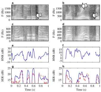
In order to qualitatively assess the effect of the two priors, a mixture of speech signals was

constructed using P=2 speech signals (a female and a male, shown in Figure 7aandb). They were

mixed through artificial channels, A, which were generated as in Section 5. Noise was added up to a level of 20dB. The EM algorithm was used to fit the source models to the mixtures. It is clear

from Figure 7c-fthat the estimated harmonic model to a large extent explains the voiced parts of the

speech signals, and the unvoiced parts to a lesser extent. In regions of rapid fundamental frequency

variation, the harmonic part cannot be fitted as well (the frames are too long here). In Figure 7g

andh, the separation performances of the AR and HN models are contrasted. Most often, the HN

performs better than the AR model. A notable exception occurs in the case when either speaker is silent, in which case the misfit of the HN model is more severe, suggesting that the performance can be improved by model control.

7. Conclusion

It is demonstrated that careful generative modelling is a viable approach to convolutive source sepa-ration and can yield improved results. Noisy observations, non-stationarity of the sources and small data volumes are examples of scenarios which benefit from the higher level of modelling detail.

The performance of the model was shown to depend on the choice of optimization scheme when the signal-to-noise ratio is high. In this case, the EM algorithm, which is often preferable for its conceptual and analytical simplicity, experiences a substantial slowdown, and alternatives must be employed. Such an alternative is a gradient-based quasi-Newton algorithm, which is shown to be particularly useful in low-noise settings. Furthermore, the required gradients are obtained in the process of deriving the EM algorithm.

The harmonic-and-noise model was investigated as a means to estimating more accurately a number of speech source signals from the their mixtures. Although a substantial improvement is shown to result when the sources are truly harmonic, the overall model is vulnerable to overfitting when the energy of one or more sources is locally near-zero. An improvement of the existing framework would be a model control scheme, such as variational Bayes, which could potentially cancel the negative impact of speaker silence. This is a topic for future research.

Acknowledgments

LINEARSTATE-SPACEMODELS FORBLINDSOURCESEPARATION

F

(Hz)

F

(Hz)

HNR

(dB)

Time (s)

SER

(dB)

F

(Hz)

F

(Hz)

HNR

(dB)

Time (s)

SER

(dB)

0 0.2 0.4 0.6 0.8 1 0 0.2 0.4 0.6 0.8 1

15 20 25 -5 0 5 10 15 0 200 400 600 800 0 500 1000 1500

15 20 25 -10 0 10 20 30 0 200 400 600 800 0 500 1000

1500 I

II II

a b

c d

e f

g h

Figure 7: The source parameters of the autoregressive (AR) and harmonic-and-noisy (HN) models

were estimated from Q=2 convolutive mixtures using the EM algorithm. Spectrograms

show the low-frequent parts of the original female (a) and male (b) speech sources. The

appropriateness of the HN model can be assessed in c and d, which displays the

re-synthesization of the two sources from the parameters (K=6), as well aseandf, where

the estimated ratio of harmonics to noise (HNR) is displayed. Overall the fit seem good, except at rapid variations of the fundamental frequency, for example, at (I), where the analysis frames are too long. The relative separation performance of the AR and HN

models, which is shown ing andh for the two sources, confirms that the HN model is

superior in most cases, with a notable exception in regions such as (II), where one of the speakers is silent. This implies a model complexity mismatch which is more severe for the more complex HN model.

Appendix A.

Below, an example of an M-step update derivation is shown for Fn. As a by-product of the

analy-sis, the derivative for the gradient-based optimizers appears. Care must be devised in obtaining the

derivatives, since Fnis a structured matrix, for example, certain elements are one and zero.

indexed by the block identifier, n, are Gaussian, we have that:

J

(θ) = −1

2

N

∑

n=1

h P

∑

i=1

n

log|Σn_i|+D sn_i,1−µn_iT(Σn_i)−1 sn_i,1−µn_i

Eo

+(T−1)

P

∑

i=1

log qn_i + 1

qn_i

T

∑

t=2

P

∑

i=1

sn_i,t−(fn

i)Tsni,t−1

2

+T log det R+

T

∑

t=1

D

(x_tn−Asn_t)TR−1(xn_t −Asn_t)E i.

The vector derivative of

J

(θ)with respect to fn_i is:

d

J

(θ)

dfn_i = 1 qn_i

"

T

∑

t=2

D

sn_i,t−1 sn_i,t−1> E

fn_i −

T

∑

t=2

sn_i,t−1sn_i,t

# .

This was the desired gradient, which is directly applicable in a gradient-based algorithm. By equat-ing to zero and solvequat-ing, the M-step update is derived:

fn_i,new=

"

T

∑

t=2

D

sn_i,t−1 sn_i,t−1> E

#−1

T

∑

t=2

sn_i,t−1sn_i,t.

References

J. Allen and D. A. Berkley. Image method for efficiently simulating small-room acoustics. Journal of the Acoustical Society of America, 65:943–950, 1979.

J. Anem¨uller and B. Kollmeier. Amplitude modulation decorrelation for convolutive blind source separation. In Proc. ICA 2000, pages 215–220, 2000.

A J. Bell and T. J. Sejnowski. An information-maximization approach to blind separation and blind deconvolution. Neural Computation, 7(6):1129–1159, 1995.

O. Bermond and J.-F. Cardoso. Approximate likelihood for noisy mixtures. In Proc. ICA, pages 325–330, 1999.

M. Brandstein. On the use of explicit speech modeling in microphone array applications. In Proc. ICASSP, pages 3613–3616, 1998.

J.-F. Cardoso, H. Snoussi, J. Delabrouille, and G. Patanchon. Blind separation of noisy Gaussian stationary sources. Application to cosmic microwave background imaging. In Proc. EUSIPCO, pages 561–564, 2002.

J. F. Cardoso and A. Souloumiac. Blind beamforming for non-gaussian signals. IEE Proceedings F, 140(6):362–370, 1993.

A. P. Dempster, N. M. Laird, and D. B. Rubin. Maximum likelihood from incomplete data via the EM algorithm. Journal of Royal Statistics Society, Series B, 39:1–38, 1977.

M. Dyrholm and L. K. Hansen. CICAAR: Convolutive ICA with an auto-regressive inverse model. In Proc. ICA 2004, pages 594–601, 2004.

P. A. Højen-Sørensen, Ole Winther, and Lars Kai Hansen. Mean-field approaches to independent component analysis. Neural Computation, 14(4):889–918, 2002.

A. Hyvarinen, J. Karhunen, and E. Oja. Independent Component Analysis. John Wiley & Sons, Inc, 2001.

R. E. Kalman and R. S. Bucy. New results in linear filtering and prediction theory. Journal of Basic Engineering ASME Transactions, 83:95–107, 1960.

T.W. Lee, A. J. Bell, and R. H. Lambert. Blind separation of delayed and convolved sources. In Advances of Neural Information Processing Systems, volume 9, page 758, 1997.

R.J. McAulay and T.F. Quateri. Speech analysis/synthesis based on a sinusoidal representation. IEEE Trans. on Acoustics, Speech and Signal Processing, 34(4):744–754, 1986.

M. McKeown, L.K. Hansen, and T.J. Sejnowski. Independent component analysis for fmri: What is signal and what is noise? Current Opinion in Neurobiology, 13(5):620–629, 2003.

E. Moulines, J. Cardoso, and E. Cassiat. Maximum likelihood for blind separation and deconvo-lution of noisy signals using mixture models. In Proc. ICASSP, volume 5, pages 3617–3620, 1997.

H. B. Nielsen. UCMINF - an algorithm for unconstrained nonlinear optimization. Technical Report IMM-Rep-2000-19, Technical University of Denmark, 2000.

R. K. Olsson and L. K. Hansen. A harmonic excitation state-space approach to blind separation of speech. In Advances in Neural Information Processing Systems, volume 17, pages 993–1000, 2005.

R. K. Olsson and L. K. Hansen. Blind separation of more sources than sensors in convolutive mixtures. In International Conference on Acoustics, Speech and Signal Processing, 2006.

R. K. Olsson, K. B. Petersen, and T. Lehn-Schiøler. State-space models - from the EM algorithm to a gradient approach. Neural Computation - to appear, 2006.

L. Parra and C. Spence. Convolutive blind separation of non-stationary sources. IEEE Transactions, Speech and Audio Processing, pages 320–7, 5 2000.

B. A. Pearlmutter and L. C. Parra. A context-sensitive generalization of ICA. In In Advances in Neural Information Processing Systems 9, pages 613–619, 1997.

H. Robbins and S. Monro. A stochastic approximation method. Annals of Mathematical Statistics, 22(3):400–407, 1951.

S. Roweis and Z. Ghahramani. A unifying review of linear Gaussian models. Neural Computation, 11:305–345, 1999.

R. Salakhutdinov and S. Roweis. Adaptive overrelaxed bound optimization methods. In Interna-tional Conference on Machine Learning, pages 664–671, 2003.

R. Salakhutdinov, S. T. Roweis, and Z. Ghahramani. Optimization with EM and Expectation-Conjugate-Gradient. In International Conference on Machine Learning, volume 20, pages 672– 679, 2003.

R. Shumway and D. Stoffer. An approach to time series smoothing and forecasting using the EM algorithm. J. Time Series Anal., 3(4):253–264, 1982.

E. Weinstein, M. Feder, and A. V. Oppenheim. Multi-channel signal separation by decorrelation. IEEE Transactions on Speech and Audio Processing, 1(4), 1993.