Handling Missing Values when Applying Classification Models
Maytal Saar-Tsechansky [email protected]
The University of Texas at Austin 1 University Station
Austin, TX 78712, USA
Foster Provost [email protected]
New York University 44West 4th Street
New York, NY 10012, USA
Editor: Rich Caruana
Abstract
Much work has studied the effect of different treatments of missing values on model induction, but little work has analyzed treatments for the common case of missing values at prediction time. This paper first compares several different methods—predictive value imputation, the distribution-based imputation used by C4.5, and using reduced models—for applying classification trees to instances with missing values (and also shows evidence that the results generalize to bagged trees and to logistic regression). The results show that for the two most popular treatments, each is preferable under different conditions. Strikingly the reduced-models approach, seldom mentioned or used, consistently outperforms the other two methods, sometimes by a large margin. The lack of attention to reduced modeling may be due in part to its (perceived) expense in terms of computation or storage. Therefore, we then introduce and evaluate alternative, hybrid approaches that allow users to balance between more accurate but computationally expensive reduced modeling and the other, less accurate but less computationally expensive treatments. The results show that the hybrid methods can scale gracefully to the amount of investment in computation/storage, and that they outperform imputation even for small investments.
Keywords: missing data, classification, classification trees, decision trees, imputation
1. Introduction
In many predictive modeling applications, useful attribute values (“features”) may be missing. For example, patient data often have missing diagnostic tests that would be helpful for estimating the likelihood of diagnoses or for predicting treatment effectiveness; consumer data often do not include values for all attributes useful for predicting buying preferences.
Although we show some evidence that our results generalize to other induction algorithms, we focus on classification trees. Classification trees are employed widely to support decision-making under uncertainty, both by practitioners (for diagnosis, for predicting customers’ preferences, etc.) and by researchers constructing higher-level systems. Classification trees commonly are used as stand-alone classifiers for applications where model comprehensibility is important, as base clas-sifiers in classifier ensembles, as components of larger intelligent systems, as the basis of more complex models such as logistic model trees (Landwehr et al., 2005), and as components of or tools for the development of graphical models such as Bayesian networks (Friedman and Goldszmidt, 1996), dependency networks (Heckerman et al., 2000), and probabilistic relational models (Getoor et al., 2002; Neville and Jensen, 2007). Furthermore, when combined into ensembles via bagging (Breiman, 1996), classification trees have been shown to produce accurate and well-calibrated prob-ability estimates (Niculescu-Mizil and Caruana, 2005).
This paper studies the effect on prediction accuracy of several methods for dealing with missing features at prediction time. The most common approaches for dealing with missing features involve
imputation (Hastie et al., 2001). The main idea of imputation is that if an important feature is
missing for a particular instance, it can be estimated from the data that are present. There are two main families of imputation approaches: (predictive) value imputation and distribution-based
imputation. Value imputation estimates a value to be used by the model in place of the missing
feature. Distribution-based imputation estimates the conditional distribution of the missing value, and predictions will be based on this estimated distribution. Value imputation is more common in the statistics community; distribution-based imputation is the basis for the most popular treatment used by the (non-Bayesian) machine learning community, as exemplified by C4.5 (Quinlan, 1993).
An alternative to imputation is to construct models that employ only those features that will be known for a particular test case—so imputation is not necessary. We refer to these models as
reduced-feature models, as they are induced using only a subset of the features that are available
for the training data. Clearly, for each unique pattern of missing features, a different model would be used for prediction. We are aware of little prior research or practice using this method. It was treated to some extent in papers (discussed below) by Schuurmans and Greiner (1997) and by Friedman et al. (1996), but was not compared broadly to other approaches, and has not caught on in machine learning research or practice.
The contribution of this paper is twofold. First, it presents a comprehensive empirical compari-son of these different missing-value treatments using a suite of benchmark data sets, and a follow-up theoretical discussion. The empirical evaluation clearly shows the inferiority of the two common imputation treatments, highlighting the underappreciated reduced-model method. Curiously, the predictive performance of the methods is more-or-less in inverse order of their use (at least in AI work using tree induction). Neither of the two imputation techniques dominates cleanly, and each provides considerable advantage over the other for some domains. The follow-up discussion exam-ines the conditions under which the two imputation methods perform better or worse.
2. Treatments for Missing Values at Prediction Time
Little and Rubin (1987) identify scenarios for missing values, pertaining to dependencies between the values of attributes and the missingness of attributes. Missing Completely At Random (MCAR) refers to the scenario where missingness of feature values is independent of the feature values (ob-served or not). For most of this study we assume missing values occur completely at random. In discussing limitations below, we note that this scenario may not hold for practical problems (e.g., Greiner et al., 1997a); nonetheless, it is a general and commonly assumed scenario that should be understood before moving to other analyses, especially since most imputation methods rely on MCAR for their validity (Hastie et al., 2001). Furthermore, Ding and Simonoff (2006) show that the performance of missing-value treatments used when training classification trees seems unrelated to the Little and Rubin taxonomy, as long as missingness does not depend on the class value (in which case unique-value imputation should be used, as discussed below, as long as the same relationship will hold in the prediction setting).
When features are missing in test instances, there are several alternative courses of action.
1. Discard instances: Simply discarding instances with missing values is an approach often taken by researchers wanting to assess the performance of a learning method on data drawn from some population. For such an assessment, this strategy is appropriate if the features are missing completely at random. (It often is used anyway.) In practice, at prediction time, discarding instances with missing feature values may be appropriate when it is plausible to decline to make a prediction on some cases. In order to maximize utility it is necessary to know the cost of inaction as well as the cost of prediction error. For the purpose of this study we assume that predictions are required for all test instances.
2. Acquire missing values. In practice, a missing value may be obtainable by incurring a cost, such as the cost of performing a diagnostic test or the cost of acquiring consumer data from a third party. To maximize expected utility one must estimate the expected added utility from buying the value, as well as that of the most effective missing-value treatment. Buying a missing value is only appropriate when the expected net utility from acquisition exceeds that of the alternative. However, this decision requires a clear understanding of the alternatives and their relative performances—a motivation for this study.
3. Imputation. As introduced above, imputation is a class of methods by which an estimation of the missing value or of its distribution is used to generate predictions from a given model. In particular, either a missing value is replaced with an estimation of the value or alternatively the distribution of possible missing values is estimated and corresponding model predictions are combined probabilistically. Various imputation treatments for missing values in histori-cal/training data are available that may also be deployed at prediction time. However, some treatments such as multiple imputation (Rubin, 1987) are particularly suitable to induction. In particular, multiple imputation (or repeated imputation) is a Monte Carlo approach that generates multiple simulated versions of a data set that each are analyzed and the results are combined to generate inference. For this paper, we consider imputation techniques that can
be applied to individual test cases during inference.1
(a) (Predictive) Value Imputation (PVI): With value imputation, missing values are replaced with estimated values before applying a model. Imputation methods vary in complexity. For example, a common approach in practice is to replace a missing value with the at-tribute’s mean or mode value (for real-valued or discrete-valued attributes, respectively) as estimated from the training data. An alternative is to impute with the average of the
values of the other attributes of the test case.2
More rigorous estimations use predictive models that induce a relationship between the available attribute values and the missing feature. Most commercial modeling packages offer procedures for predictive value imputation. The method of surrogate splits for classification trees (Breiman et al., 1984) imputes based on the value of another feature, assigning the instance to a subtree based on the imputed value. As noted by Quinlan (1993), this approach is a special case of predictive value imputation.
(b) Distribution-based Imputation (DBI). Given a (estimated) distribution over the values of an attribute, one may estimate the expected distribution of the target variable (weighting the possible assignments of the missing values). This strategy is common for applying classification trees in AI research and practice, because it is the basis for the miss-ing value treatment implemented in the commonly used tree induction program, C4.5 (Quinlan, 1993). Specifically, when the C4.5 algorithm is classifying an instance, and a test regarding a missing value is encountered, the example is split into multiple pseudo-instances each with a different value for the missing feature and a weight corresponding to the estimated probability for the particular missing value (based on the frequency of values at this split in the training data). Each pseudo-instance is routed down the ap-propriate tree branch according to its assigned value. Upon reaching a leaf node, the class-membership probability of the pseudo-instance is assigned as the frequency of the class in the training instances associated with this leaf. The overall estimated probability of class membership is calculated as the weighted average of class membership proba-bilities over all pseudo-instances. If there is more than one missing value, the process recurses with the weights combining multiplicatively. This treatment is fundamentally different from value imputation because it combines the classifications across the dis-tribution of an attribute’s possible values, rather than merely making the classification based on its most likely value. In Section 3.3 we will return to this distinction when analyzing the conditions under which each technique is preferable.
(c) Unique-value imputation. Rather than estimating an unknown feature value it is possible to replace each missing value with an arbitrary unique value. Unique-value imputation is preferable when the following two conditions hold: the fact that a value is missing depends on the value of the class variable, and this dependence is present both in the training and in the application/test data (Ding and Simonoff, 2006).
4. Reduced-feature Models: Imputation is required when the model being applied employs an attribute whose value is missing in the test instance. An alternative approach is to apply a dif-ferent model—one that incorporates only attributes that are known for the test instance. For
example, a new classification tree could be induced after removing from the training data the features corresponding to the missing test feature. This reduced-model approach may poten-tially employ a different model for each test instance. This can be accomplished by delaying model induction until a prediction is required, a strategy presented as “lazy” classification-tree induction by Friedman et al. (1996). Alternatively, for reduced-feature modeling one may store many models corresponding to various patterns of known and unknown test features.
With the exception of C4.5’s method, dealing with missing values can be expensive in terms of storage and/or prediction-time computation. In order to apply a reduced-feature model to a test example with a particular pattern P of missing values, it is necessary either to induce a model for
P on-line or to have a model for P precomputed and stored. Inducing the model on-line involves
computation time3 and storage of the training data. Using precomputed models involves storing
models for each P to be addressed, which in the worst case is exponential in the number of attributes. As we discuss in detail below, one could achieve a balance of storage and computation with a hybrid method, whereby reduced-feature models are stored for the most important patterns; lazy learning or imputation could be applied for less-important patterns.
More subtly, predictive imputation carries a similar expense. In order to estimate the missing value of an attribute A for a test case, a model must be induced or precomputed to estimate the value of A based on the case’s other features. If more than one feature is missing for the test case, the imputation of A is (recursively) a problem of prediction with missing values. Short of abandoning straightforward imputation, one possibility is to take a reduced-model approach for
imputation itself, which begs the question: why not simply use a direct reduced-model approach?4
Another approach is to build one predictive imputation model for each attribute, using all the other features, and then use an alternative imputation method (such as mean or mode value imputation, or C4.5’s method) for any necessary secondary imputations. This approach has been taken previously (Batista and Monard, 2003; Quinlan, 1989), and is the approach we take for the results below.
3. Experimental Comparison of Prediction-time Treatments for Missing Values
The following experiments compare the predictive performance of classification trees using value imputation, distribution-based imputation, and reduced-feature modeling. For induction, we first employ the J48 algorithm, which is the Weka (Witten and Frank, 1999) implementation of C4.5 classification tree induction. Then we present results using bagged classification trees and logistic regression, in order to provide some evidence that the findings generalize beyond classification trees. Our experimental design is based on the desire to assess the relative effectiveness of the differ-ent treatmdiffer-ents under controlled conditions. The main experimdiffer-ents simulate missing values, in order to be able to know the accuracy if the values had been known, and also to control for various con-founding factors, including pattern of missingness (viz., MCAR), relevance of missing values, and induction method (including missing value treatment used for training). For example, we assume that missing features are “important”: that to some extent they are (marginally) predictive of the class. We avoid the trivial case where a missing value does not affect prediction, such as when a feature is not incorporated in the model or when a feature does not account for significant variance
3. Although as Friedman et al. (1996) point out, lazy tree induction need only consider the single path in the tree that matches the test case, leading to a considerable improvement in efficiency.
in the target variable. In the former case, different treatments should result in the same classifica-tions. In the latter case different treatments will not result in significantly different classificaclassifica-tions. Such situations well may occur in practical applications; however, the purpose of this study is to assess the relative performance of the different treatments in situations when missing values will af-fect performance, not to assess how well they will perform in practice on any particular data set—in which case, careful analysis of the reasons for missingness must be undertaken.
Thus, we first ask: assuming the induction of a high-quality model, and assuming that the values of relevant attributes are missing, how do different treatments for missing test values compare? We then present various followup studies: using different induction algorithms, using data sets with “naturally occurring” missing values, and including increasing numbers missing values (chosen at random). We also present an analysis of the conditions under which different missing value treatments are preferable.
3.1 Experimental Setup
In order to focus on relevant features, unless stated otherwise, values of features from the top two levels of the classification tree induced with the complete feature set are removed from test instances (cf. Batista and Monard, 2003). Furthermore, in order to isolate the effect of various treatments for dealing with missing values at prediction time, we build models using training data having no missing values, except for the natural-data experiments in Section 3.6.
For distribution-based imputation we employ C4.5’s method for classifying instances with miss-ing values as described above. For value imputation we estimate missmiss-ing categorical features usmiss-ing a J48 tree, and continuous values using Weka’s linear regression. As discussed above, for value imputation with multiple missing values we use mean/mode imputation for the additional missing values. For generating a reduced model, for each test instance with missing values, we remove all the corresponding features from the training data before the model is induced so that only features that are available in the test instance are included in the model.
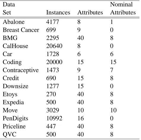
Each reported result is the average classification accuracy of a missing-value treatment over 10 independent experiments in which the data set is randomly partitioned into training and test sets. Except where we show learning curves, we use 70% of the data for training and the remaining 30% as test data. The experiments are conducted on fifteen data sets described in Table 1. The data sets comprise web-usage data sets (used by Padmanabhan et al., 2001) and data sets from the UCI machine learning repository (Merz et al., 1996).
To conclude that one treatment is superior to another, we apply a sign test with the null hy-pothesis that the average drops in accuracy using the two treatments are equal, as compared to the complete setting (described next).
3.2 Comparison of PVI, DBI and Reduced Modeling
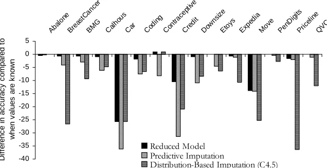
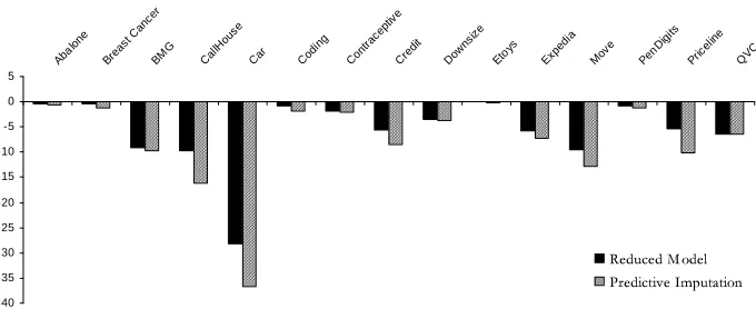
Figure 1 shows the relative difference for each data set and each treatment, between the classification accuracy for the treatment and (as a baseline) the accuracy obtained if all features had been known both for training and for testing (the “complete” setting). The relative difference (improvement) is given by 100·ACT−ACK
ACK , where ACK is the prediction accuracy obtained in the complete setting, and
ACT denotes the accuracy obtained when a test instance includes missing values and a treatment T
Data Nominal
Set Instances Attributes Attributes
Abalone 4177 8 1
Breast Cancer 699 9 0
BMG 2295 40 8
CalHouse 20640 8 0
Car 1728 6 6
Coding 20000 15 15
Contraceptive 1473 9 7
Credit 690 15 8
Downsize 1277 15 0
Etoys 270 40 8
Expedia 500 40 8
Move 3029 10 10
PenDigits 10992 16 0
Priceline 447 40 8
QVC 500 40 8
Table 1: Summary of Data Sets
values degrade classification, even when the treatments are used. Small negative values in Figure 1 are better, indicating that the corresponding treatment yields only a small reduction in accuracy.
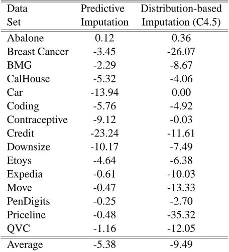
Reduced-feature modeling is consistently superior. Table 2 shows the differences in the relative improvements obtained with each imputation treatment from those obtained with reduced modeling. A large negative value indicates that an imputation treatment resulted in a larger drop in accuracy than that exhibited by reduced modeling.
Reduced models yield an improvement over one of the other treatments for every data set. The reduced-model approach results in better performance compared to distribution-based imputation in 13 out of 15 data sets, and is better than value imputation in 14 data sets (both significant with
p<0.01).
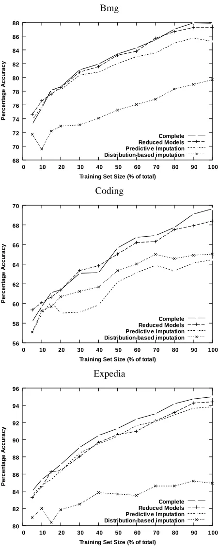
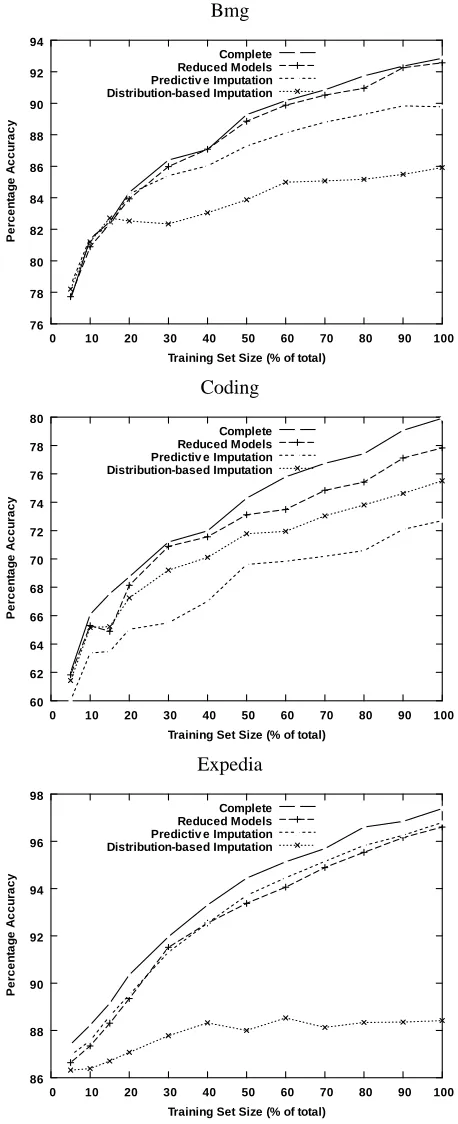
Not only does a reduced-feature model almost always result in statistically significantly more-accurate predictions, the improvement over the imputation methods often was substantial. For ex-ample, for the Downsize data set, prediction with reduced models results in less than 1% decrease in accuracy, while value imputation and distribution-based imputation exhibit drops of 10.97% and 8.32%, respectively; the drop in accuracy resulting from imputation is more than 9 times that ob-tained with a reduced model. The average drop in accuracy obob-tained with a reduced model across all data sets is 3.76%, as compared to an average drop in accuracy of 8.73% and 12.98% for predictive imputation and distribution-based imputation, respectively. Figure 2 shows learning curves for all treatments as well as for the complete setting for the Bmg, Coding and Expedia data sets, which show three characteristic patterns of performance.
3.3 Feature Imputability and Modeling Error
-40 -35 -30 -25 -20 -15 -10 -5 0 5 Aba lone Bre astC ance r BM G Cal hous
Car Cod
ing Con trace ptiv e Cre dit Dow nsiz e Eto ys Exp edia Mov e Pen Dig its Pric elin e QV C D if fe re n c e i n a c c u ra c y c o m p a re d t o w h e n v a lu e s a re k n o w n Reduced Model P r edi ct i v e I m p ut a t i on
D i s t r i b ut i on - B a s ed I m p ut a t i on ( C 4 . 5 )
Figure 1: Relative differences in accuracy (%) between prediction with each missing data treatment and prediction when all feature values are known. Small negative values indicate that the treatment yields only a small reduction inaccuracy. Reduced modeling consistently yields the smallest reductions in accuracy—often performing nearly as well as having all the data. Each of the other techniques performs poorly on at least one data set, suggesting that one should choose between them carefully.
imputation (PVI) and C4.5’s distribution-based imputation (DBI), each has a stark advantage over the other in some domains. Since to our knowledge the literature currently provides no guidance as to when each should be applied, we now examine conditions under which each technique ought to be preferable.
The different imputation treatments differ in how they take advantage of statistical dependencies between features. It is easy to develop a notion of the exact type of statistical dependency under which predictive value imputation should work, and we can formalize this notion by defining feature
imputability as the fundamental ability to estimate one feature using others. A feature is completely
imputable if it can be predicted perfectly using the other features—the feature is redundant in this sense. Feature imputability affects each of the various treatments, but in different ways. It is reveal-ing to examine, at each end of the feature imputability spectrum, the effects of the treatments on
expected error.5 In Section 3.3.4 we consider why reduced models should perform well across the
spectrum.
3.3.1 HIGHFEATUREIMPUTABILITY
First let’s consider perfect feature imputability. Assume also, for the moment, that both the primary modeling and the imputation modeling have no intrinsic error—in the latter case, all existing feature
Data Predictive Distribution-based
Set Imputation Imputation (C4.5)
Abalone 0.12 0.36
Breast Cancer -3.45 -26.07
BMG -2.29 -8.67
CalHouse -5.32 -4.06
Car -13.94 0.00
Coding -5.76 -4.92
Contraceptive -9.12 -0.03
Credit -23.24 -11.61
Downsize -10.17 -7.49
Etoys -4.64 -6.38
Expedia -0.61 -10.03
Move -0.47 -13.33
PenDigits -0.25 -2.70
Priceline -0.48 -35.32
QVC -1.16 -12.05
Average -5.38 -9.49
Table 2: Differences in relative improvement (from Figure 1 between each imputation treatment and reduced-feature modeling. Large negative values indicate that a treatment is substan-tially worse than reduced-feature modeling
imputability is captured. Predictive value imputation simply fills in the correct value and has no effect whatsoever on the bias and variance of the model induction.
Consider a very simple example comprising two attributes, A and B, and a class variable C with
A=B=C. The “model” A→C is a perfect classifier. Now given a test case with A missing,
predictive value imputation can use the (perfect) feature imputability directly: B can be used to infer A, and this enables the use of the learned model to predict perfectly. We defined feature imputability as a direct correlate to the effectiveness of value imputation, so this is no surprise. What is interesting is now to consider whether DBI also ought to perform well. Unfortunately, perfect feature imputability introduces a pathology that is fatal to C4.5’s distribution-based imputation. When using DBI for prediction, C4.5’s induction may have substantially increased bias, because it omits redundant features from the model—features that will be critical for prediction when the alternative features are missing. In our example, the tree induction does not need to include variable
B because it is completely redundant. Subsequently when A is missing, the inference has no other
features to fall back on and must resort to a default classification. This was an extreme case, but note that it did not rely on any errors in training.
Bmg 68 70 72 74 76 78 80 82 84 86 88
0 10 20 30 40 50 60 70 80 90 100
P e rc e n ta g e A c c u ra c y
Training Set Size (% of total) Complete Reduced Models Predictiv e Imputation Distribution-based imputation Coding 56 58 60 62 64 66 68 70
0 10 20 30 40 50 60 70 80 90 100
P e rc e n ta g e A c c u ra c y
Training Set Size (% of total) Complete Reduced Models Predictiv e Imputation Distribution-based imputation Expedia 80 82 84 86 88 90 92 94 96
0 10 20 30 40 50 60 70 80 90 100
P e rc e n ta g e A c c u ra c y
Training Set Size (% of total) Complete Reduced Models Predictiv e Imputation Distribution-based imputation
A
A=1, 30% A=3, 30%
B B
B
90% -10% +
20% -80% +
70% -30% +
90% -10% +
B=1, 50% B=0, 50%
B=1, 50% B=0, 50%
70% -30% +
90% -10% +
B=1, 50% B=0, 50%
A=2, 40%
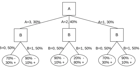
Figure 3: Classification tree example: consider an instance at prediction time for which feature A is unknown and B=1.
Finally, consider the inference procedures under high imputability. With PVI, classification trees’ predictions are determined (as usual) based on the class distribution of a subset Q of training examples assigned to the same leaf node. On the other hand, DBI is equivalent to classification based on a superset S of Q. When feature imputability is high and PVI is accurate, DBI can only do as well as PVI if the weighted majority class for S is the same as that of Q. Of course, this is not always the case so DBI should be expected to have higher error when feature imputability is high.
3.3.2 LOWFEATUREIMPUTABILITY
When feature imputability is low we expect a reversal of the advantage accrued to PVI by using Q rather than S. The use of Q now is based on an uninformed guess: when feature imputability is very low PVI must guess the missing feature value as simply the most common one. The class estimate obtained with DBI is based on the larger set S and captures the expectation over the distribution of missing feature values. Being derived from a larger and unbiased sample, DBI’s “smoothed” estimate should lead to better predictions on average.
As a concrete example, consider the classification tree in Figure 3. Assume that there is no feature imputability at all (note that A and B are marginally independent) and assume that A is missing at prediction time. Since there is no feature imputability, A cannot be inferred using B and
the imputation model should predict the mode (A=2). As a result every test example is passed to the
A=2 subtree. Now, consider test instances with B=1. Although (A=2, B=1) is the path chosen
by PVI, it does not correspond to the majority of training examples with B=1. Assuming that test
instances follow the same distribution as training instances, on B=1 examples PVI will have an
Difference between Value Imputation and DBI
-13.00 -3.00 7.00 17.00 27.00 37.00
Car Cre
dit
Cal Hous
e
Cod ing
Con trace
ptiv e
Mov e
Dow nsiz
e
BcW isc Bmg
Abal one Etoys
PenD igits
Expe dia
Pric elin
e Qvc
Low Feature Imputability High
Figure 4: Differences between the relative performances of PVI and DBI. Domains are ordered left-to-right by increasing feature imputability. PVI is better for higher feature imputability, and DBI is better for lower feature imputability.
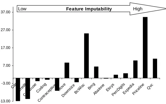
3.3.3 DEMONSTRATION
Figure 4 shows the 15 domains of the comparative study ordered left-to-right by a proxy for
in-creasing feature imputability.6 The bars represent the differences in the entries in Table 2, between
predictive value imputation and C4.5’s distribution-based imputation. A bar above the horizontal line indicates that value imputation performed better; a bar below the line indicates that DBI per-formed better. The relative performances follow the above argument closely, with value imputation generally preferable for high feature imputability, and C4.5’s DBI generally better for low feature imputability.
3.3.4 REDUCED-FEATUREMODELINGSHOULDHAVEADVANTAGESALLALONG THE
IMPUTABILITYSPECTRUM
Whatever the degree of imputability, reduced-feature modeling has an important advantage. Re-duced modeling is a lower-dimensional learning problem than the (complete) modeling to which imputation methods are applied; it will tend to have lower variance and thereby may exhibit lower
generalization error. To include a variable that will be missing at prediction time at best adds an irrelevant variable to the induction, increasing variance. Including an important variable that would be missing at prediction time may be worse, because unless the value can be replaced with a highly accurate estimate, its inclusion in the model is likely to reduce the effectiveness at capturing predic-tive patterns involving the other variables, as we show below.
In contrast, imputation takes on quite an ambitious task. From the same training data, it must build an accurate base classifier and build accurate imputation models for any possible missing values. One can argue that imputation tries implicitly to approximate the full-joint distribution, similar to a graphical model such as a dependency network (Heckerman et al., 2000). There are many opportunities for the introduction of error, and the errors will be compounded as imputation models are composed.
Revisiting the A,B,C example of Section 3.3.1, reduced-feature modeling uses the feature
im-putability differently from predictive imputation. The (perfect) feature imim-putability ensures that
there will be an alternative model (B→C) that will perform well. Reduced-feature modeling may
have additional advantages over value imputation when the imputation is imperfect, as just dis-cussed.
Of course, the other end of the feature imputability spectrum, when feature imputability is very low, is problematic generally when features are missing at prediction time. At the extreme, there is no statistical dependency at all between the missing feature and the other features. If the missing feature is important, predictive performance will necessarily suffer. Reduced modeling is likely to be better than the imputation methods, because of its reduced variance as described above.
Finally, consider reduced-feature modeling in the context of Figure 3, and where there is no feature imputability at all. What would happen if due to insufficient data or an inappropriate in-ductive bias, the complete modeling were to omit the important feature (B) entirely? Then, if A is missing at prediction time, no imputation technique will help us do better than merely guessing that the example belongs to the most common class (as with DBI) or guessing that the missing value is the most common one (as in PVI). Reduced-feature modeling may induce a partial (reduced) model
(e.g., B=0→C=−, B=1→C= +) that will do better than guessing in expectation.
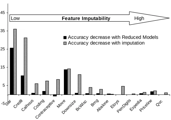
Figure 5 uses the same ordering of domains, but here the bars show the decreases in accuracy over the complete-data setting for reduced modeling and for value imputation. As expected, both techniques improve as feature imputability increases. However, the reduced-feature models are much more robust—with only one exception (Move) reduced-feature modeling yields excellent performance until feature imputability is very low. Value imputation does very well only for the domains with the highest feature imputability (for the highest-imputability domains, the accuracies of imputation and reduced modeling are statistically indistinguishable).
3.4 Evaluation using Ensembles of Trees
-5 5 15 25 35 45
Car Cre
dit Cal
hous Cod
ing
Con trace
ptiv e
Mov e
Dow nsiz
e BcW
isc Bmg Abal
one Etoy
s PenD
igits Expe
dia Pric
elin e
Qvc
Accuracy decrease with Reduced Models Accuracy decrease with imputation Low Feature Imputability High
Figure 5: Decreases in accuracy for reduced-feature modeling and value imputation. Domains are ordered left-to-right by increasing feature imputability. Reduced modeling is much more robust to moderate levels of feature imputability.
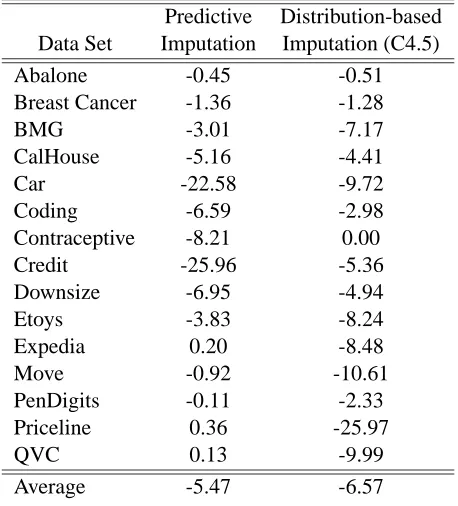
Figure 6 shows the performance of the three missing-value treatments using bagged classifica-tion trees, showing (as above) the relative difference for each data set between the classificaclassifica-tion accuracy of each treatment and the accuracy of the complete setting. As with simple trees, reduced modeling is consistently superior. Table 3 shows the differences in the relative improvements of each imputation treatment from those obtained with reduced models. For bagged trees, reduced modeling is better than predictive imputation in 12 out of 15 data sets, and it performs better than distribution-based imputation in 14 out of 15 data sets (according to the sign test, these differences
are significant at p<0.05 and p<0.01 respectively). As for simple trees, in some cases the
advan-tage of reduced modeling is striking.
Figure 7 shows the performance of all treatments for models induced with an increasing training-set size for the Bmg, Coding and Expedia data training-sets. As for single classification models, the advan-tages obtained with reduced models tend to increase as the models are induced from larger training sets.
These results indicate that for bagging, a reduced model’s relative advantage with respect to predictive imputation is comparable to its relative advantage when a single model is used. These results are particularly notable given the widespread use of classification-tree induction, and of bagging as a robust and reliable method for improving classification-tree accuracy via variance reduction.
-40 -35 -30 -25 -20 -15 -10 -5 0 5
Abal one
Brea st C
ance r
BM G
Cal lHou
se
Car Cod ing
Con trace
ptiv e
Cre dit
Dow nsiz
e
Etoy s
Expe dia
Mov e
PenD igits
Pric elin
e
QV C
!
"#$%!&' (# !*)+-,/.01
Figure 6: Relative differences in accuracy for bagged decision trees between each missing value treatment and the complete setting where all feature values are known. Reduced modeling consistently is preferable. Each of the other techniques performs poorly on at least one data set.
Predictive Distribution-based
Data Set Imputation Imputation (C4.5)
Abalone -0.45 -0.51
Breast Cancer -1.36 -1.28
BMG -3.01 -7.17
CalHouse -5.16 -4.41
Car -22.58 -9.72
Coding -6.59 -2.98
Contraceptive -8.21 0.00
Credit -25.96 -5.36
Downsize -6.95 -4.94
Etoys -3.83 -8.24
Expedia 0.20 -8.48
Move -0.92 -10.61
PenDigits -0.11 -2.33
Priceline 0.36 -25.97
QVC 0.13 -9.99
Average -5.47 -6.57
Table 3: Relative difference in prediction accuracy for bagged decision trees between imputation treatments and reduced-feature modeling.
3.5 Evaluation using Logistic Regression
Bmg 76 78 80 82 84 86 88 90 92 94
0 10 20 30 40 50 60 70 80 90 100
P e rc e n ta g e A c c u ra c y
Training Set Size (% of total) Complete Reduced Models Predictiv e Imputation Distribution-based Imputation Coding 60 62 64 66 68 70 72 74 76 78 80
0 10 20 30 40 50 60 70 80 90 100
P e rc e n ta g e A c c u ra c y
Training Set Size (% of total) Complete Reduced Models Predictiv e Imputation Distribution-based Imputation Expedia 86 88 90 92 94 96 98
0 10 20 30 40 50 60 70 80 90 100
P e rc e n ta g e A c c u ra c y
Training Set Size (% of total) Complete Reduced Models Predictiv e Imputation Distribution-based Imputation
-40 -35 -30 -25 -20 -15 -10 -5 0 5
Aba lone
Brea st C
ance r
BM G
Cal lHou
se
Car Cod ing
Con trace
ptiv e
Cre dit
Dow nsiz
e
Etoy s
Expe dia
Mov e
Pen Dig
its
Pric elin
e
QVC
! "
Figure 8: Relative differences in accuracies for a logistic regression model when predicitve value imputation and reduced modeling are employed, as compared to when all values are known.
Because C4.5-style distribution-based imputation is not applicable for logistic regression, we com-pare predictive value imputation to the reduced model approach. Figure 8 shows the difference in accuracy when predictive value imputation and reduced models are used. Table 4 shows the differ-ences in the relative improvements of the predictive imputation treatment from those obtained with reduced models. For logistic regression, reduced modeling results in higher accuracy than predictive
imputation in all 15 data sets (statistically significant with p0.01).
3.6 Evaluation with “Naturally Occurring” Missing Values
We now compare the treatment on four data sets with naturally occurring missing values. By “nat-urally occurring,” we mean that these are data sets from real classification problems, where the missingness is due to processes of the domain outside of our control. We hope that the compari-son will provide at least a glimpse at the generalizability of our findings to real data. Of course, the missingness probably violates our basic assumptions. Missingness is unlikely to be completely at random. In addition, missing values may have little or no impact on prediction accuracy, and the corresponding attributes may not even be used by the model. Therefore, even if the qualitative results hold, we should not expect the magnitude of the effects to be as large as in the controlled studies.
Predictive
Data Set Imputation
Abalone -0.20
Breast Cancer -1.84
BMG -0.75
CalHouse -7.11
Car -12.04
Coding -1.09
Contraceptive -1.49
Credit -3.05
Downsize -0.32
Etoys -0.26
Expedia -1.59
Move -3.68
PenDigits -0.34
Priceline -5.07
QVC -0.02
Average -2.59
Table 4: Relative difference in prediction accuracy for logistic regression between imputation and reduced-feature modeling. Reduced modeling never is worse, and sometimes is substan-tially more accurate.
Data Nominal Average Number
Set Instances Attributes Attributes of Missing Features
Hospitalization 48083 13 7 1.73
Insurance 18542 16 0 2.32
Mortgage 2950 10 1 2.76
Pricing 15531 28 8 3.56
Table 5: Summary of business data sets with “naturally occurring” missing values.
Figure 9 and Table 6 show the relative decreases in classification accuracy that result for each treatment relative to using a reduced-feature model. These results with natural missingness are con-sistent with those obtained in the controlled experiments discussed earlier. Reduced modeling leads to higher accuracies than both popular alternatives for all four data sets. Furthermore, predictive value imputation and distribution-based imputation each outperforms the other substantially on at least one data set—so one should not choose between them arbitrarily.
3.7 Evaluation with Multiple Missing Values
-4 -3.5 -3 -2.5 -2 -1.5 -1 -0.5 0
Hospitalization Insurance Mortgage Pricing
! "$#%&'
Figure 9: Relative percentage-point differences in predictive accuracy obtained with distribution-based imputation and predictive value imputation treatments compared to that obtained with reduced-feature models. The reduced models are more accurate in every case.
Predictive Distribution-based
Data Set Imputation Imputation (C4.5)
Hospitalization -0.52 -2.27
Insurance -3.04 -3.03
Mortgage -3.40 -0.74
Pricing -1.82 -0.48
Table 6: Relative percentage-point difference in prediction accuracy between imputation treatments and reduced-feature modeling.
at inference time. Performance may also be undermined when a large number of feature values are missing at inference time.
Figure 10 shows the accuracies of reduced-feature modeling and predictive value imputation as the number of missing features increases, from 1 feature up to when only a single feature is left. Features are removed at random. The top graphs are for tree induction and the bottom for bagged tree induction. These results are for Breast Cancer and Coding, which have moderate-to-low feature imputability, but the general pattern is consistent across the other data sets. We see a typical pattern: the imputation methods have steeper decreases in accuracy as the number of missing values increases. Reduced modeling’s decrease is convex, with considerably more robust performance even for a large number of missing values.
50 52 54 56 58 60 62 64 66 68 70
0 2 4 6 8 10 12 14
P e rc e n ta g e A c c u ra c y
Number of missing features Reduced model Distribution-based imputation Predictiv e Imputation
65 70 75 80 85 90 95
1 2 3 4 5 6 7 8
P e rc e n ta g e A c c u ra c y
Number of missing features Reduced model Distribution-based imputation Predictiv e Imputation
Coding (Single tree) Breast Cancer (Single tree)
45 50 55 60 65 70 75 80
0 2 4 6 8 10 12 14
P e rc e n ta g e A c c u ra c y
Number of missing features Reduced model Distribution-based imputation Predictiv e Imputation
20 30 40 50 60 70 80 90 100
1 2 3 4 5 6 7 8
P e rc e n ta g e A c c u ra c y
Number of missing features Reduced model Distribution-based imputation Predictiv e Imputation
Coding (Bagging) Breast Cancer (Bagging)
Figure 10: Accuracies of missing value treatments as the number of missing features increases
categorical features (viz., Car, Coding, and Move, for which we use C4.5 for both the base model and the imputation model), we see the same patterns of results as with the other data sets.
4. Hybrid Models for Efficient Prediction with Missing Values
4.1 Likelihood-based Hybrid Solutions
One approach for reducing the computational cost of reduced modeling is to induce and store mod-els for some subset of the possible patterns of missing features. When a test case is encountered, the corresponding reduced model is queried. If no corresponding model has been stored, the hy-brid would call on a fall-back technique: either incurring the expense of prediction-time reduced modeling, or invoking an imputation method (and possibly incurring reduced accuracy).
Not all patterns of missing values are equally likely. If one can estimate from prior experience the likelihood for any pattern of missing values, then this information may be used to decide among different reduced models to induce and store. Even if historical data are not sufficient to support accurate estimation of full, joint likelihoods, it may be that the marginal likelihoods of different variables being missing are very different. And even if the marginals are or must be assumed to be uniform, they still may well lead to very different (inferred) likelihoods of the many patterns of multiple missing values. In the context of Bayesian network induction, Greiner et al. (1997b) note the important distinction between considering only the underlying distribution for model induc-tion/selection and considering the querying distribution as well. Specifically, they show that when comparing different Bayesian networks one should identify the network exhibiting the best expected performance over the query distribution, that is, the distribution of tasks that the network will be used to answer, rather than the network that satisfies general measures such as maximum likelihood over the underlying event distribution. H. and F. (1992) employ a similar notion to reduce inference time with Bayesian networks. H. and F. (1992) precompute parts of the network that pertain to a subset of frequently encountered cases so as to increase the expected speed of inference.
The horizontal, dashed line in Figure 11 shows the performance of pure predictive value impu-tation for the CalHouse data set. The lower of the two curves in Figure 11 shows the performance of a likelihood-based reduced-models/imputation hybrid. The hybrid approach allows one to choose an appropriate space-usage/accuracy tradeoff, and the figure shows that storing even a few reduced models can result in considerable improvement. The curve was generated as follows. Given enough space to store k models, the hybrid induces and stores reduced models for the top-k most likely missing-feature patterns, and uses distribution-based imputation for the rest. The Calhouse data set has eight attributes, corresponding to 256 patterns of missing features. We assigned a random probability of occurrence for each pattern as follows. The frequency of each pattern was drawn at random from the unit uniform distribution and subsequently normalized so that the frequencies added up to one. For each test instance we sampled a pattern from the resulting distribution and removed the values of features specified by the pattern.
68 69 70 71 72 73 74 75 76 77 78 79
0 50 100 150 200 250 300
Num ber of m odels induced (for hybrid approaches )
C
la
s
s
if
ic
a
ti
o
n
A
c
c
u
ra
c
y
Reduced Models/Imputation Hybrid Prediction with Imputation Expected Utility
Figure 11: Accuracies of hybrid strategies for combining reduced modeling and imputation. Stor-ing even a small fraction of the possible reduced models can improve accuracy consid-erably.
even if it weren’t, the optimization problem is hard. Specifically, the optimal set of reduced models
M corresponds to solving the following optimization task:
argmaxM ∑
f
[p(f)·U(f |M)] !
s.t. ∑ fm∈M
t(fm)≤T ,
where M is the subset of missing patterns for which reduced models are induced, t(f) is the
(marginal) resource usage (time or space) for reduced modeling with pattern f , T is the
maxi-mum total resource usage allocated for reduced model induction, and U(f|M) denotes the utility
from inference for an instance with pattern f given the set of reduced models in the subset M (when
f ∈M the utility is derived from inference via the respective reduced model, otherwise the utility is
derived from inference using the next-best already-stored pattern).
The upper curve in Figure 11 shows the performance of a heuristic approximation to a utility-maximizing hybrid. We estimate the marginal utility of adding a missing-feature pattern f as
u(f) = p(f)·(aˆrm(f)−aˆi(f)), where p(f) is the likelihood of encountering pattern f , ˆarm(f) is
the estimated accuracy of reduced modeling for f and ˆai(f)is the estimated accuracy of a
predic-tive value imputation model for missing pattern f . We estimate ˆarm(f)and ˆai(f)based on
cross-validation using the training data. The figure shows that even a heuristic expected-utility approach can improve considerably over the pure likelihood-based approach.
4.2 Reduced-Feature Ensembles
Reduced-Feature Ensemble (ReFE), based on a set
R
of models each induced by excluding a singleattribute, where the cardinality of
R
is the number of attributes. Model i∈R
tries to capture analternative hypothesis that can be used for prediction when the value for attribute vi, perhaps among
others, is unknown. Because the models exclude only a single attribute, a ReFE avoids the com-binatorial space requirement of full-blown reduced modeling. When multiple values are missing, ReFE ensemble members rely on imputation for the additional missing values. We employ DBI.
More precisely, a ReFE classifier works as follows. For each attribute vi a model mi is induced
with vi removed from the training data. For a given test example in which the values for the set
of attributes V are missing, for each attribute vi ∈V whose value is missing, the corresponding
model miis applied to estimate the (probability of) class membership. To generate a prediction, the
predictions of all models applied to a test example are averaged. When a single feature is missing, ReFE is identical to the reduced-model approach. The application of ReFE for test instances with two or more missing features results in an ensemble. Hence, in order to achieve variance reduction as with bagging, in our experiments training data are resampled with replacement for each member of the ensemble.
Table 7 summarizes the relative improvements in accuracy as compared to a single model using predictive value imputation. For comparison we show the improvements obtained by bagging alone (with imputation), and by the full-blown reduced-model approach. For these experiments we fixed the number of missing features to be three. The accuracies of ReFE and bagging are also plotted in Figure 12 to highlight the difference in performance across domains. Bagging uses the same number of models as employed by ReFE, allowing us to separate the advantage that can be attributed to the reduced modeling and that attributable to variance reduction.
We see that ReFE consistently improves over both a single model with imputation (positive en-tries in the ReFE column) and over bagging with imputation. In both comparisons, ReFE results in higher accuracy on all data sets, shown in bold in Table 7, except Car; the 14-1 win-loss record is
statistically significant with p<0.01. The magnitudes of ReFE’s improvements vary widely, but on
average they split the difference between bagging with imputation and the full-blown reduced mod-eling. Note that although full-blown reduced modeling usually is more accurate, ReFE sometimes shows better accuracy, indicating that the variance reduction of bagging complements the (partial) reduced modeling.
The motivation for employing ReFE instead of the full-blown reduced-feature modeling is the substantially lower computational burden of ReFE as compared to that of reduced modeling. For a
domain with N attributes,(2N−1)models must be induced by reduced modeling in order to match
each possible missing pattern. ReFE induces only N models—one for each attribute. For example, the Calhouse data set, which includes only 8 attributes, required more than one-half hour to produce all the 256 models for full-blown reduced modeling. It took about a minute to produce the 8 models for the ReFE.
4.3 Larger Ensembles
Reduced
Data Sets Bagging ReFE Model
Abalone 0.11 0.26 0.05
BreastCancer 4.35 4.51 4.62
Bmg 2.88 3.51 2.57
CalHouse 1.25 6.06 5.45
Car 0.10 -0.28 17.55
Coding 4.82 6.97 5.32
Contraceptive 0.39 0.45 1.16
Credit 2.58 5.54 8.12
Downsize 3.09 3.78 6.51
Etoys 0.00 2.28 1.07
Expedia 1.76 2.11 2.73
Move 3.26 5.99 8.97
Pendigits 0.06 0.58 1.57
Priceline 3.29 4.98 10.84
Qvc 1.83 2.44 2.60
Average 1.98 3.27 5.27
Table 7: Relative improvements in accuracy for bagging with imputation and ReFE, as compared to a single model with imputation. Bold entries show the cases where ReFE improves both over using a single model with imputation and over bagging with imputation. For compar-ison, the rightmost column shows the improvements of full-blown reduced modeling. The ReFEs are more accurate than either a single model with imputation, or bagging with im-putation, while being much more efficient than reduced modeling in terms of computation and/or storage.
For control, for any given number of missing features in a test example, we evaluate the performance of bagging with the same number of individual models. Similarly, we generate a bagged version of the full-blown reduced model, with the same number of models as in the other approaches. As before, we fix the number of missing values in each test instance to three.
As expected, including a larger number of models in each ensemble results in improved perfor-mance for all treatments, for almost all data sets. The advantage exhibited by ReFE over bagging with imputation is maintained. As shown in Table 8. ReFE results in higher accuracy than bagging
with imputation for all 15 data sets (statistically significant at p0.01).
4.4 ReFEs with Increasing Numbers of Missing Values
-1 0 1 2 3 4 5 6 7 8 Aba lone Bre astC ance r Bm g Cal Hou
se Car
Cod ing Con trace ptiv e Cre dit Dow nsiz e Eto ys Exp edia Mov
e Pen digi ts Pric elin e QV C R e la it v e I m p ro v e m e n t in A c c u ra c y
Figure 12: Relative improvement in accuracy (%) as obtained for bagging with imputation and ReFE, with respect to a single model with imputation.
Bagging with Bagging with
Data Sets Imputation ReFE Reduced Model
Abalone 0.34 0.49 0.83
BreastCancer 5.10 5.89 5.15
Bmg 7.22 7.88 8.21
CalHouse 2.66 7.10 8.47
Car -0.10 -0.08 17.55
Coding 14.39 15.28 17.65
Contraceptive 0.64 0.89 1.03
Credit 4.98 6.77 9.35
Downsize 6.91 7.60 11.13
Etoys 2.95 3.35 3.48
Expedia 3.41 4.19 5.27
Move 6.48 9.73 13.78
PenDigits 0.44 0.90 1.52
Priceline 7.55 9.42 11.02
QVC 4.23 5.88 7.16
Average 4.48 5.69 8.11
Table 8: Percentage improvement in accuracy compared to a single model with imputation, for bagging with imputation, ReFE, and bagging with reduced models. All ensembles employ 30 models for prediction. Bold entries show the cases where ReFE improves both over using a single model with imputation and over bagging with imputation.
60 65 70 75 80 85
0 2 4 6 8 10 12
P e rc e n ta g e A c c u ra c y
Number of missing features Reduced Models
ReFE Imputation-Bagging Imputation - Tree
56 58 60 62 64 66 68 70 72 74
2 3 4 5 6 7 8
P e rc e n ta g e A c c u ra c y
Number of missing features Reduced Models
ReFE Imputation-Bagging Imputation - Tree
Credit Move
Figure 13: Performance of missing value treatments for small ensemble models as the number of missing values increases.
60 65 70 75 80 85
0 2 4 6 8 10 12
Accurac y ging - ! "# els $ E
ging with Imputation
56 58 60 62 64 66 68 70 72 74 76 78
2 3 4 5 6 7 8
P e rc e n ta g e A c c u ra c y
Number of missing features Bagging- Reduced Models
ReFE Bagging w ith Imputation
Credit Move
Figure 14: Performance of treatments for missing values for large ensemble models as the number of missing values increases.
values. For the larger ensembles, Figure 14 shows the classification accuracies for ReFE, bagging with imputation, and bagging with reduced models, where each ensemble includes 30 models. In general, the patterns observed for small ensembles are exhibited for larger ensembles as well.
In sum, while using no more storage space than standard bagging, ReFE offers significantly better performance than imputation and than bagging with imputation for small numbers of missing values and hence provides another alternative for domains where full-blown reduced modeling (and especially reduced modeling with bagging) is impracticably expensive. Thus, in domains in which test instances with few missing values are frequent it may be beneficial to consider the use of ReFE, resorting to reduced modeling only for (infrequent) cases with many missing values.
on the tradeoff spectrum, by incorporating more reduced models. As in Section 4.1 we face a difficult optimization problem, and various heuristic approximations come to mind (e.g., somehow combining the models selected for storage in Section 4.1 ).
5. Related Work
Although value imputation and distribution-based imputation are common in practical applications of classification models, there is surprisingly little theoretical or empirical work analyzing the strate-gies. The most closely related work is the theoretical treatment by Schuurmans and Greiner’s (1993) within the PAC framework (Valiant, 1984). The present paper can be seen in part as an empirical complement to their theoretical treatment. Schuurmans and Greiner consider an “attribute blocking” process in which attribute values are not available at induction time. The paper discusses instances of the three strategies we explore here: value imputation (simple default-value imputation in their paper), distribution-based prediction, and a reduced-feature “classifier lattice” of models for all pos-sible patterns of missing values. For the missing completely at random scenario, they discuss that reduced-feature modeling is the only technique that is unconditionally consistent (i.e., is always guaranteed to converge to the optimal classifier in the large-data limit).
Our experimental results support Schuurmans and Greiner’s assertion that under some condi-tions it is beneficial to expose the learner to the specific pattern of missing values observed in a test instance (reduced modeling), rather than to “fill in” a missing value. Our analysis gives insight into the underlying factors that lead to this advantage, particularly in terms of the statistical dependencies among the predictor variables.
Empirical work on handling missing values has primarily addressed the challenge of induction from incomplete training data (e.g., Rubin, 1987; Dempster et al., 1977; Schafer, 1997; Batista and Monard, 2003; Feelders, 1999; Ghahramani and Jordan, 1994, 1997). For example, Ghahramani and Jordan (1997) assume an explicit probabilistic model and a parameter estimation procedure and present a framework for handling missing values during induction when mixture models are estimated from data. Specifically for classification trees, Quinlan (1993) studies joint treatments for induction and prediction with missing nominal feature values. The study explores two forms of
imputation similar to those explored here7and classification by simply using the first tree node for
which the feature is missing (treating it as a leaf); the study does not consider reduced-feature mod-els. Quinlan concludes that no solution dominates across domains. However, C4.5’s DBI seems to
perform best more often and hence the paper recommends its use.8 Our study revealed the opposite
pattern—predictive value imputation often is superior to C4.5’s DBI. More importantly, however, we show that the dominance of one form of imputation versus another depends on the statistical de-pendencies (and lack thereof) between the features: value imputation is likely to outperform C4.5’s DBI when feature imputability is particularly high, and vice versa.
Porter et al. (1990) propose a heuristic classification technique (Protos) for weak-theory do-mains. In contrast to the induction of an abstract generalization, Protos learns concepts by retaining exemplars, and new instances are classified by matching them with exemplars. Porter et al. apply
7. Predictive value imputation was implemented by imputing either the mode value or a prediction using a decision tree classifier.
Protos, ID3, and another exemplar-based program to a medical diagnosis problem where more than 50% of the test feature values are missing, and where missingness depends on the feature values (e.g., yes/no features were always missing when the true value is “no”). They note that because of the large proportion of missing values, ID3 with various imputation techniques performed poorly. Our empirical results show a similar pattern.
To our knowledge very few studies have considered reduced-feature modeling. Friedman et al. (1996) propose the induction of lazy classification trees, an instance of run-time reduced modeling. They induce single classification-tree paths that are tailored for classifying a particular test instance, thereby not incorporating any missing features. When classifying with missing values, Friedman et al. report the performance of lazy tree induction to be superior to C4.5’s technique. Explain-ing the results, the authors note that “avoidExplain-ing any tests on unknown values is the correct thExplain-ing to do probabilistically, assuming the values are truly unknown...” Our study supports this argument and complements it by showing how the statistical dependencies exhibited by relevant features are either exploited or ignored by each approach. For example, our followup analysis suggests that C4.5’s technique will have particular difficulty when feature imputability is high, as it is for many benchmark data sets. Ling et al. (2004) examine strategies to reduce the total costs of feature-value acquisitions and of misclassifications; they employ lazy tree induction and show similar results to Friedman et al. Neither paper considers value imputation as an alternative, nor do they explore the domain characteristics that enable the different missing-value treatments to succeed or fail. For ex-ample, our followup analysis shows that with high feature imputability, predictive value imputation can perform just as well as lazy (reduced-feature) modeling, but reduced modeling is considerably more robust to lower levels of imputability.
We described how reduced modeling may take advantage of alternative predictive patterns in the training data. Prior work has noted the frequent availability of such alternative predictive patterns, and suggests that these can be exploited to induce alternative hypotheses. In particular, co-training (Blum and Mitchell, 1998) is an induction technique that relies on the assumption that the feature set comprises two disjoint subsets such that each is sufficient to induce a classifier, and that the features in each set are not highly correlated with those of the other conditional on the class. Blum and Mitchell offer web pages as an example for alternative representations, in which a page can be represented by its content or by the words occurring in hyperlinks that point to that page. Each representation can be used to induce models of comparable performance. Nigam and Ghani (2000) show that co-training is often successful because alternative representations are rather common. Specifically, Nigam and Ghani demonstrate that even for data sets for which such a natural partition does not exist, a random partition usually produces two sets that are each sufficient for accurate classification. Our empirical results for reduced models provide additional evidence that alternative feature subsets can be used effectively. Hence, accurate reduced models can frequently be induced in practice and offer an alternative that consistently is at least comparable to and usually superior to popular treatments.
6. Limitations
unre-lated to the Little and Rubin taxonomy, as long as missingness does not depend on the class value (Ding and Simonoff, 2006).
Schuurmans and Greiner (1997) consider the other end of the spectrum, missingness being a completely arbitrary function of an example’s values, and conclude that none of the strategies we consider will be consistent (albeit one may perform better than another consistently in practice). However, there is a lot of ground between MCAR and completely arbitrary missingness. In the “missing at random” (MAR) scenario (Little and Rubin, 1987) missingness is conditioned only on observed values. For example, a physician may decide not to conduct one diagnostic test on the basis of the result of another. Presumably, reduced modeling would work well for MAR, since two examples with the same observed features will have the same statistical behavior on the unobserved features. If features are “missing not at random” (MNAR), there still may be useful subclasses. As a simple example, if only one particular attribute value is ever omitted (e.g., “Yes” to “Have you committed a felony?”), then unique-value imputation should work well. Practical application would benefit from a comprehensive analysis of common cases of missingness and their implications for using learned models.
Although we show some evidence of generalizability with logistic regression, our study was primarily limited to classification trees (and ensembles of trees). As noted at the outset, trees are very common both alone—especially when comprehensibility is a concern—and as components of ensembles, more sophisticated models, and larger inference systems. Some of the arguments apply to many model types, for example that reduced modeling will have lower variance. Others are spe-cific to C4.5’s DBI (which of course in the artificial intelligence and machine learning literatures is a widely used and cited missing-value treatment). C4.5’s DBI is not based on an estimation of the full, joint distribution—the lack of which is the basis for the pathology presented in Section 3.3.1. How-ever, full-joint methods also have practical drawbacks: they are very expensive computationally, can be intractable for large problems, and they are awkward for practitioners (and for researchers) in comparison to simpler classification/regression methods. Nevertheless, extending beyond classi-fication trees, it would be well to consider DBI based on a full-joint model. (And it should be noted that naive Bayes marginalizes simply by ignoring attributes with missing values, so treatments such as these are unnecessary.)
Imputation may be more (or less) effective if we were to use other classification and regression methods. However, our arguments supporting the results are not limited a particular imputation model. In the case of multiple missing values, we have not analyzed the degree to which imputation would improve if a reduced-modeling approach were taken for the imputation itself, rather than using simple value imputation. We see no justification for doing so rather than simply using reduced modeling directly.
We avoid, as beyond the scope of this paper, the complicated question of whether there are notable interactions between the missing value treatment used at induction time and the missing value treatment used when the resultant models are applied.